Generalized Hampel Filters

(1)

EURASIP Journal on Advances

in Signal Processing

Pearsonet al. EURASIP Journal on Advances in Signal

Processing (2016) 2016:87 DOI 10.1186/s13634-016-0383-6

R E S E A R C H

Open Access

Generalized Hampel Filters

Ronald K. Pearson

1*

, Yrjö Neuvo

2

, Jaakko Astola

3

and Moncef Gabbouj

3

Abstract

The standard median filter based on a symmetric moving window has only one tuning parameter: the window width. Despite this limitation, this filter has proven extremely useful and has motivated a number of extensions: weighted median filters, recursive median filters, and various cascade structures. TheHampel filteris a member of the class of decsion filters that replaces the central value in the data window with the median if it lies far enough from the median to be deemed an outlier. This filter depends on both the window width and an additional tuning parametert, reducing to the median filter whent=0, so it may be regarded as another median filter extension. This paper adopts this view, defining and exploring the class ofgeneralized Hampel filtersobtained by applying the median filter

extensions listed above: weighted Hampel filters, recursive Hampel filters, and their cascades. An important concept introduced here is that of animplosion sequence, a signal for which generalized Hampel filter performance is independent of the threshold parametert. These sequences are important because the added flexibility of the generalized Hampel filters offers no practical advantage for implosion sequences. Partial characterization results are presented for these sequences, as are useful relationships between root sequences for generalized Hampel filters and their median-based counterparts. To illustrate the performance of this filter class, two examples are considered: one is simulation-based, providing a basis for quantitative evaluation of signal recovery performance as a function oft, while the other is a sequence of monthly Italian industrial production index values that exhibits glaring outliers.

1 Introduction

In their paper, “On a class of nonlinear filters,” Sicuranza and Carini begin by noting [1]:

“The set of nonlinear filters is extremely large since their definition simply excludes the applicability of the linear superposition property on which the theory of linear filters is based. However, from the very

beginning, attempts have been done to suitably classify nonlinear filters on the basis of some peculiar

properties, leading to the identification of certain classes of nonlinear filters.”

This paper adopts a similar philosophy, restricting con-sideration to a class of nonlinear filters obtained by com-bining two previously studied filter classes: theHampel filterdescribed in Section 2, and the median filter exten-sions described in Sections 4 and 7. The result is a class of nonlinear filters we believe to be new, that includes all of these previously studied filters as special cases, but which exhibits a greater degree of design flexibility.

*Correspondence: [email protected] 1DataRobot, Inc., Boston MA, USA

Full list of author information is available at the end of the article

2 Standard median and Hampel filters

All of the filters discussed in this paper are based on the following moving data window, or some simple extension of it:

WK_k = {xk−K,. . .,xk,. . .,xk+K}, (1)

where K is a positive integer called the window half-width. Thestandard median filterMK was introduced by J.W. Tukey in 1974 [2] and is obtained by computing the median of the moving data windowWK_k:

mk =median{xk−K,. . .,xk,. . .,xk+K}. (2)

The only tuning parameter for this filter is the window half-width parameter K, which limits its flexibility, but the real strength of the median filter lies in its extreme resistance tolocal outliersorimpulsive noisein the input data squence {xk}. Unfortunately, the median filter can also introduce significant distortion in the portion of the signal we wish to retain, making its utility strongly application-dependent. These filter characteristics have led to the development of a number of median filter exten-sions, including the recursive median filter discussed in Section 4 and others described in Section 7.

(2)

A closely related filter is theHampel filter HK, which belongs to the class ofdecision-based filtersdiscussed in the book by Astola and Kuosmanen ([3] p. 194), who note that the basic concept has been reinvented again and again. The version considered here represents a moving-window implementation of theHampel identifier

described by Davies and Gather [4], an outlier detec-tion procedure based on the median and the MAD scale estimator. Specifically, this filter’s response is given by:

yk =

xk |xk−mk| ≤tSk,

mk |xk−mk|>tSk. (3)

where mk is the median value from the moving data

window andSkis the MAD scale estimate, defined as:

Sk=1.4826×medianj∈[−K,K]{|xk−j−mk|}. (4)

The factor 1.4826 makes the MAD scale estimate an unbiased estimate of the standard deviation for Gaussian data.

The key observation on which this paper is based is that, when the threshold parametertis set to zero, we recover the standard median filter:

yk|t=0=mk. (5)

It follows from this observation that we may regard the Hampel filter as a generalization of the median filter, with

tas an additional tuning parameter. The central question explored in this paper is what the consequences of this generalization are when we combine it with other gener-alizations of the median filter that are well-known in the literature, as described in Sections 4 and 7.

A filter’s root sequences are those sequences {xk} that are invariant under the action of the filter, and the root squences for the standard median filter have been well-characterized (see, for example [5] or [6]). Thus, it is worth noting that the set Rt of root sequences for the Hampel filter with thresholdtcontains the median filter root sequence R0for allt ≥ 0. Specifically, ifs ≤ t, it follows that:

|xk−mk| ≤sSk≤tSk ⇒ Rs⊂Rt. (6)

The practical implication of this result is that the Hampel filter may be viewed as a “less aggressive exten-sion” of the median filter, generally becoming less aggres-sive with increasing threshold value t. In particular, for “most” sequences{xk}, the Hampel filter varies from the median filter at is most aggressive (i.e., fort = 0) to an identity filter as t → ∞. The important exception to this behavior is the class ofimplosion sequencesdescribed next.

3 Implosion sequences

The MAD scale estimator has the extremely desirable characteristic of exhibiting the maximum possible outlier

resistance [4], but it does suffer from an unfortunate sen-sitivity toimplosion:if more than 50 % of the data values are the same, the MAD scale estimate is zero, indepen-dent of the other values in the data sequence. The practical consequences for the Hampel filter are that ifK +1 or more of the values in the data windowWK_k have the same value, thenSk = 0, implying thatyk = mk, independent of the threshold parametert. Thus, we make the following definitions:

1. Define the windowWK_k to be animplosion window if

Sk =0;

2. Define the sequence{xk}to be animplosion sequence if all windows are implosion windows (i.e., ifS_k=0for allk);

3. Define the sequence{xk}to beimplosion-free if it contains no implosion windows (i.e., ifSk>0for all k).

The practical consequence of these definitions is that if {xk}is an implosion sequence, the output of the Hampel filter reduces to that of the median filter for all t, so the added flexibility of the Hampel filter offers no prac-tical advantage for these sequences. Similarly, since the Hampel filter root set contains the median filter root set for all threshold values t, the added flexibility of the Hampel filter offers no practical advantage for these sequences, either.Thus, the signals of greatest interest in characterizing Hampel filter performance are implosion-free sequences that are not median filter roots.

As noted in Section 2, the Hampel filter reduces to the standard median filter when the threshold parameter has the value t = 0, and it becomes generally less aggres-sive with increasingt. It follows directly from the defining equations that the Hampel filter has no effect on the input signal if the following condition is satisfied:

max

k |xk−mk| ≤tmink Sk, (7)

where the maximum on the left-hand side and the min-imum on the right-hand side of this condition are taken over all moving data windows. If {xk} is an implosion-free sequence, it follows that minkSk > 0, so Eq. (7) can be inverted to yield the following condition for signal preservation:

t≥ maxk|xk−mk|

minkSk

. (8)

(3)

Pearsonet al. EURASIP Journal on Advances in Signal Processing (2016) 2016:87 Page 3 of 18

TheoremThe sequence{xk} is an implosion sequence forHK if and only if, for all k, more than K elements of the windowWK_k have the same value.

Proof 1. Assume{xk}is an implosion sequence for HK. This means:

median{|xk−mk|} =0,

implying|xk−mk| =0for at leastK+1values, implyingxk=mkfor at leastK+1values inWK_k. 2. Conversely, suppose that at leastK+1values inWK_k

are equal to some constantc. It follows immediately that the median value in this window ismk=c, implying|xk−mk| =0for at leastK+1values, implyingSk=0so that{xk}is an implosion sequence forHK.

This result allows us to construct some specific exam-ples of Hampel filter implosion sequences from the signal components used by Gallagher and Wise to character-ize median filter root sequences [6]. Specifically, givenK, define the following four components:

1. Aconstant neighborhood is a sequence of at least

K+1consequtive identical values;

2. Anedge is a monotonically increasing or decreasing sequence, preceeded and followed by constant neighborhoods of different values;

3. Animpulse is a sequence of at mostKvalues, preceeded and followed by constant neighborhoods having the same value, with the values of the intermediate points distinct from those of the surrounding constant neighborhoods;

4. Anoscillation is any sequence of values not contained in a constant neighborhood, an edge, or an impulse.

Based on these definitions, it can be shown that{xk}is a root sequence for the median filterMK if and only if it consists entirely of constant neighborhoods and edges [6]. Note that by the above theorem, a sequence{xk}that consists entirely of constant neighborhoods will be an implosion sequence for HK. In this case, it follows by the above result that{xk}is also a root sequence for the median filterMK, so we expect no difference in behav-ior between the median and Hampel filters for this case by the root sequence nesting condition (6). A more inter-esting example is the case of a sequence{xk} composed of constant neighborhoods and impulses. Here again, it is easy to see that this sequence is an implosion sequence forHK, but it is not a median filter root sequence. In this case, the Hampel filter will reduce to the median filter for all threshold parameterstand map{xk}to a sequence of constant neighborhoods with the impulses removed. Note

that this sequence is a median filter root sequence. Finally, a third class of implosion sequences is the class ofbinary oscillations: it follows immediately from the above theorem that{xk}is an implosion sequence forHK.

An interesting open question is whether there are other classes of implosion sequences forHK besides the three just described. Since any root sequence for the median filterMK is also a root for all Hampel filtersHK, regard-less of threshold, the important implosion sequences are those that are not median filter roots: these sequences are modified by the median filter and also modified in exactly the same way by the Hampel filter, independent of the threshold parametert.

4 Recursive median and Hampel filters

The recursive median filter is obtained by replacing the symmetric moving windowWK_k defined in Eq. (1) with the following recursive data window:

RK_k = {mk−K,. . .,mk−1,xk,xk+1,. . .,xk+K}, (10)

wheremk−jrepresents the output at prior timek−jof the standard median filter applied to the input sequence{xk}. This extension exhibits a number of interesting proper-ties, includingidempotence[7], i.e., a single application of the recursive median filter maps{xk}into the filter’s root set. Further, it has also been shown that the root set for the recursive median filter is identical to that for the standard median filter.

The recursive Hampel filter is defined analogously, replacing the recursive window defined in Eq. (10) based on prior median filter outputs, with the alternative window:

Rt_k,K = {H_kt₋_K,. . .,H_kt₋₁,xk,xk+1,. . .,xk+K}, (11)

whereH_kt₋_jrepresents the output at prior timek−jof the Hampel filter with threshold parametertapplied to the input sequence{xk}.

It follows by direct extension of the root set nesting result given in Eq. (6) for the nonrecursive case that the recursive Hampel filter root set contains the recursive median filter root set. Specifically, if{r_k}is a root for the Hampel filter with thresholdsfor 0≤s≤t, then:

|r_k₋_j−m_k₋_j| ≤sS_k₋_j≤tS_k₋_j ⇒ H_ks₋_j=H_kt₋_j=r_k₋_j. (12)

(4)

1. The recursive and non-recursive Hampel root sets are identical for every threshold parameter:R˜t=Rt for allt;

2. The recursive Hampel root sets nest: for all0≤s≤t, it follows thatR˜s⊂ ˜Rt.

Beyond these results, the following interesting questions are open at present:

1. The recursive median filter is idempotent—does this behavior extend to recursive Hampel filters for arbitraryt? If not, is the recursive median filter the only idempotent member of this family? More generally, how does idempotence depend ont? 2. What is the relationship between implosion

sequences for the recursive and non-recursive Hampel filters?

5 The influence ofton filter performance

To provide quantitative filter performance results, the fol-lowing section presents a brief case study that examines the influence of the Hampel filter tuning parameterton the performance of both the standard Hampel filter and the recursive Hampel filter. Since the primary question of interest is the influence of the tuning parametert, this example considers a fixed window half-width parameter (specifically, K = 5, yielding an 11-point moving win-dow filter) and examines filter performance over a range oftvalues. The basis for these performance comparisons is a simulated data example described in Section 5.1: the advantage of considering a simulation-based example is that we can be explicit about the signal components we wish to recover and can therefore quantify signal recovery performance. More specifically, this example considers two possible signal recovery problems described in detail in Section 5.1 and characterizes performance in terms of two metrics: the root mean square signal recovery error (RMSE) and the mean absolute signal recovery error (MAE).

5.1 A simulated data example

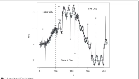
To provide a basis for comparing the different filters con-sidered in this paper, we apply them to the 420-point simulated data sequence shown in Fig. 1, which contains four components:

1. Step-and-ramp sequence (median filter root) for

k=1, 2,. . ., 420;

2. Low-level Gaussian noise (partial: nonzero only for

k=1, 2,. . ., 240);

3. Sinusoid (partial: nonzero only for

k=101, 102,. . ., 420);

4. Impulsive noise, randomly distributed throughout the sequence.

More specifically, the step-and-ramp sequence consists of eight segments:

The Gaussian noise component has mean zero and stan-dard deviationσ=0.1, and the sinusoid has period 29 and amplitude 0.3. The impulsive noise component is an addi-tive term that is zero everywhere except for the following eight values ofk, where it takes the nonzero values indi-cated in parentheses:k =20 (+1),k= 35 (−1),k= 120 (+1), k = 190 (−1.5),k = 220 (−2.5),k = 300 (+1),

k=350 (+2.5), andk=410 (+1.5).

The primary question of interest here is how well the different filters considered eliminate the isolated spikes in this signal while preserving the low-level details, espe-cially the sinusoidal component. The presence of the low-level noise in approximately the first half of the sig-nal raises a subtle practical issue, however: is a “good” filter one that simply removes the impulsive spikes from the data sequence, or should it also address the low-level noise? Given that median filters and their extensions are much better suited to the removal of impulsive noise than the smoothing of low-level noise, the first formulation seems the more reasonable here, but the question is raised to emphasize that filter performance criteria are generally problem-specific.

Additional insights can be obained from this example by considering filter performance for the three qualita-tively distinct signal subsequenes separated by dashed vertical lines in Fig. 1. Specifically, the first 100 points of the sequence—denoted “Noise Only” in Fig. 1—consists of a median filter root sequence, contaminated with both low-level Gaussian noise and impulsive noise spikes. The

second subsequence, from k = 100 to k = 240 and

labelled “Noise + Sine,” contains all four of the signal com-ponents listed above, while the third subsequence, from

k=240 tok=420 and labelled “Sine Only,” consists of a median filter root sequence with a superimposed sinusoid and isolated spikes, but no low-level noise.

The two signal recovery problems considered here are the following:

(5)

Fig. 1A simulated 420-point signal

P2 the complete noise removal problem, where the signal to be recovered consists of the sum of the two deterministic components (i.e., the median filter root plus the sinusoid), without either low-level or impulsive noise.

As noted above, these signal recovery problems have different characters, with the first being more suitable for the filter class considered here, but the second prob-lem is of considerable practical significance. Two perfor-mance measures are considered for both problems: the root-mean-square recovery error (RMSE) is more widely used, but may be less appropriate than the mean absolute recovery error (MAE) in the presence of impulsive noise.

Finally, it is important to note that, for the filter window width considered here (K=5), the signal sequence shown in Fig. 1 is implosion-free and is not a median filter root sequence. Thus, it follows that filter performance should depend on the threshold parametert, and the objective of the following discussions is to illuminate the nature of this dependence.

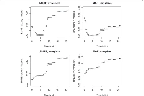
5.2 Results for the Hampel filter

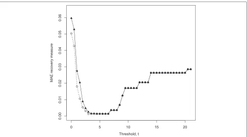
For the signal defined in Section 5.1, the identity filter threshold described in Section 3 is approximatelyt= 21, so the results presented here consider the performance of the Hampel filter over the range fromt =0 tot= 21, in increments of 0.5. Four views of the signal recovery per-formance of the Hampel filter over this range oftvalues

are presented in Fig. 2. The upper left plot shows the RMSE signal recovery measure for the impulsive noise removal problem, the upper right shows the correspond-ing MAE signal recovery measure, the lower left plot shows the RMSE measure for the complete noise removal problem, and the lower right shows the MAE measure for this problem. Note that the two RMSE plots are shown on the same scale to facilitate comparison, as are the two MAE plots, but the RMSE and MAE scales are differ-ent. For the impulsive noise removal problem (the upper two plots), both measures exhibit a broad but well-defined minimum for threshold parameterstbetween 3.0 and 6.5. For values much smaller than 3, performance degrades sharply astdecreases to thet=0 median filter limit; sim-ilarly, performance again degrades as thetvalue increases from 6.5, particularly for the RMSE measure, as the Hampel filter approaches the identity limit. The MAE view in the upper right is particularly interesting here: this performance measure is poorest for the median fil-ter, becoming consistently better than the median filter for allt ≥ 1.0. This result reflects the significant distortion introduced into the signal sequence by the median filter, offsetting its ability to remove the noise spikes.

(6)

Fig. 2Hampel filter performance vs.tby four different criteria: RMSE or MAE, impulsive noise removal or complete noise removal

noise and the low-level noise, these results suggest that as

tincreases, the Hampel filter allows more of the low-level noise to pass through the filter unmodified, offsetting the performance advantage of lower distortion of the sinu-soidal signal components. In particular, since the filter removes all of the impulsive noise spikes fortbetween 0 and 6.5, it follows that the poorer performance seen for the complete noise removal problem over the impulsive noise removal optimal performance range (t = 3.5 tot = 6.0) relative to the median filter limitt = 0 is caused by the filter’s allowing more low-level noise into the output sig-nal. These results emphasize the point made earlier that these filters are not well-suited to low-level noise removal problems.

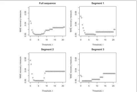
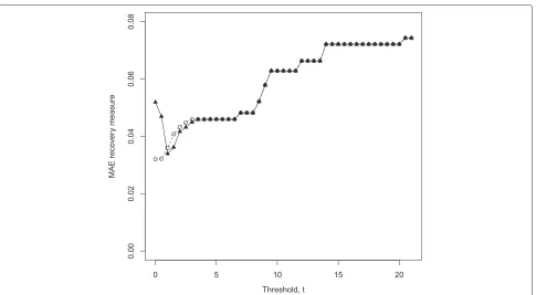
Figure 3 shows the MAE performance for the impul-sive noise removal problem as a function of t, broken down by signal segment: the upper left plot corresponds to the upper right plot in Fig. 2, characterizing the com-plete signal sequence, while the other three plots show the corresponding results for the three segments indicated in Fig. 1. The upper right plot presents the results for Seg-ment 1 (“Noise only”), consisting of the median filter root sequence, low-level Gaussian noise, and impulsive noise

spikes. This plot clearly shows the low-level noise dis-tortion effects for smallt values, which is worst for the median filter (t =0), decreasing monotonically untilt =

3.0, where the filter is sufficiently non-aggressive to allow most of the low-level noise through unmodified. In fact, the optimal filter performance for this signal sequence occurs att=8.5 where the MAE is near zero. Fort≥9.5, the filter begins allowing impulsive noise spikes into the output, causing a dramatic increase in MAE. The lower left plot in Fig. 3 shows the results for Segment 2 (“Noise + Sine”). As in Segment 1, the performance is worst for the median filter, improving uniformly with increasingt

(7)

Fig. 3Hampel filter MAE performance vs.tfor impulsive noise removal: full sequence (upper left), Segment 1 (upper right), Segment 2 (lower left), and Segment 3 (lower right)

beyond this limit, the filter begins to pass impulsive noise spikes, becoming an identity filter fort≥14.0.

Figure 4 shows a plot of the median filter response (t=

0, represented by open circles), overlaid with a solid line representing the response of the Hampel filter witht=5, falling in the optimal parameter range for the complete signal and all segments except Segment 1, where the per-formance is near-optimal. In addition, points where these two filter responses differ are indicated by solid rectan-gles. From these results, it is clear that the Hampel filter witht = 5 passes both the low-level noise components and the sinusolidal components essentially perfectly, while the median filter seriously distorts the portions of the sig-nal contaminated with low-level noise, and it “clips” the tops and bottoms of the sinusoidal component. It is also clear that both filters remove all of the impulsive noise from the signal sequence.

The frequency of the sinusoidal component in this example is important. Specifically, the maximum possi-ble frequency is that of the binary implosion sequence described in Section 3, implying that in this limit, the Hampel filter offers no advantage over the median filter. At the other extreme, if the sinusoidal frequency is low

enough, theN-point finite signal sequence will be mono-tonic, and thus a root sequence for the median filter and all Hampel filters. For intermediate frequencies; however, sinusoidal components are neither implosion sequences nor roots, and as this example illustrates, the response of the Hampel filter to these components generally varies strongly witht.

5.3 Results for the recursive Hampel filter

Figure 5 shows the complete sequence performance for the recursive Hampel filter. Specifically, the upper left

plot shows the RMSE measure versus t for the

(8)

Fig. 4Median filter response (open circles) and Hampel filter response witht₌5 (lines), with points of disagreement marked assolid squares

(9)

Fig. 6Recursive (solid triangles) and non-recursive (open circles) Hampel filter MAE performance vs.tfor impulsive noise removal

reached, after which the two filter responses appear to be identical.

The more interesting results in Fig. 5 are the two bot-tom plots for the complete noise removal problem: in contrast to the monotonic behavior seen in the corre-sponding plots in Fig. 2, the recursive filter exhibits a sharp optimum att = 1. A more detailed comparison of the recursive and nonrecursive Hampel filter MAE per-formance is shown in Fig. 7: for small t, the recursive filter performance is much worse than the standard filter, although fort values between 1.0 and 3.0, the recursive filter actually performs slightly better; for largertvalues, both filters exhibit essentially identical performance.

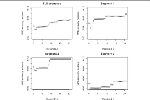
Figure 8 summarizes the recursive median filter’s MAE performance for the complete noise removal problem as a function oftfor the complete signal and the three seg-ments marked in Fig. 1. The upper left plot shows the results for the complete signal and is the same as the lower right plot in Fig. 5, included here to facilitate visual comparisons. The upper right plot shows the results for Segment 1 (“Noise only”) and here, the optimum att=1 is much sharper than that for the complete signal, with performance degrading much more rapidly astincreases beyond this value. The results for Segment 2 (“Noise + sine”) shown in the lower left plot are a bit more compli-cated: optimal performance is again obtained fort = 1, but this optimum is shallower than that for Segment 1 and there is a second, small local minimum fromt=2.5 tot=

3, after which performance again degrades monotonically

with increasingt. Finally, the performance for Segment 3 (“Sine only”, lower right plot) is virtually identical to that seen for the standard Hampel filter shown in the lower right plot in Fig. 3.

Overall, these results—particularly those for the com-plete noise removal performance of the recursive Hampel filter—show that the performance of these filters depends strongly on the threshold valuet, but very differently for different signal extraction problems and different signal characteristics. For example, for Segment 3 (“Sine only”), the performance of the recursive and standard Hampel filters are almost identical, both for the impulse noise removal problem and for the complete noise removal problem: distortion is observed fortless than 1.0, excel-lent performance is observed fortbetween 1.0 and 6.5, with consistent performance degradation astis increased beyond this value. In contrast, for Segment 1 (“Noise only”), these performance curves are very different: for the impulsive noise removal problem with the standard Hampel filter, performance is worst in the median filter limit, improves uniformly as tincreases to 3.5 where it

remains near-optimal as t increases to 8.5; optimal

performance—only slightly better—is achieved for t

(10)

Fig. 7Recursive (solid triangles) and non-recursive (open circles) Hampel filter MAE performance vs.tfor complete noise removal

as t increases, exhibiting worse performance than the recursive median filter for all t > 2. Finally, as noted, the complete noise removal performance for the recur-sive Hampel filter for Segment 2 (“Noise + sine”) is even more complicated, exhibiting local optima in its MAE vs.

tperformance curve.

6 A real data example

To provide an illustration of how the generalized Hampel filters described in this paper work with a real data exam-ple, the following section applies several of these filters to a publically-available time-series dataset. Specifically, this example is based on the gipi sequence included in the tsoutliers R package [8], available as one row of the

bde9915 data frame. This data sequence is a monthly time-series of Italian industrial production index from 1981 to 1996, consisting of 192 observations. A plot of this time-series is shown in Fig. 9, from which the pres-ence of significant outliers in the data is clear. In fact, these anomalous data points occur at regular 12-month intervals and represent what Kaiser and Maravall call sea-sonal outliers[9]. If we apply standard time-series mod-eling procedures (e.g., fitting ARMA or ARIMA models to the data), the results will be profoundly influenced by the presence of these outliers, and at least two general strategies can be used to address these problems. The first is the development of specialized analysis procedures

that are resistant to the anomalies in the data, extending standard analysis methods using fundamental ideas from robust statistics, such as the robust time-series model-ing approach described by Martin and Yohai [10] or the robust-resistant spectrum estimation approach described by Martin and Thomson [11]. The second approach is the use of simple data-cleaning filters like those described in this paper to remove the outliers from the data sequence, after which standard analysis procedures are applied. The primary objective of this example is to illustrate the range of results that may be obtained when different general-ized Hampel filters are applied to the time-series shown in Fig. 9.

Figure 10 shows the results of two standard median fil-ters (upper two plots) and two recursive median filfil-ters (lower two plots) applied to the Italian industrial produc-tion data shown in Fig. 9. The left-hand plots correspond to filters based on the window half-width parameterK =

(11)

Fig. 8Recursive Hampel filter MAE performance vs.tfor complete noise removal: full sequence (upper left), Segment 1 (upper right), Segment 2 (lower left), and Segment 3 (lower right)

recursive median filters. It is also clear that the distortion introduced by these filters is worse forK=5 than it is for

K=3.

Figure 11 shows comparative results for four different Hampel-based filters. As in Fig. 10, the top two plots are for nonrecursive Hampel filters, while the bottom two plots are for their recursive counterparts. Here, all of these filters are based on the half-width parameter K = 5, with the right- and left-hand plots differing in the Ham-pel threshold parametert. Specifically, the left-hand plots correspond to the more aggressive threshold valuet =1, while the right-hand plots are based ont = 2. As before, all of these filters completely eliminate the seasonal out-liers from the data, introducing much less distortion in the nominal part of the signal than the corresponding median filters do. Comparing the left-hand and right-hand plots, it is also clear that these filters introduce much less distor-tion witht=2 than witht=1. Comparing the upper and lower plots, it is also clear that while the recursive Ham-pel filter introduces more nominal signal distortion than the nonrecursive filter for this signal, this effect becomes much less pronounced with increasingt.

One type of generalized Hampel filter that was not dis-cussed in connection with the simulation example was the subclass of cascade interconnections of Hampel fil-ters and/or recursive Hampel filfil-ters. Figure 12 shows the results obtained when four different filter cascades are applied to the Italian industrial production index data shown in Fig. 9. In the upper left plot, the results were obtained by first applying the standard median filter with

(12)

Fig. 9Monthly Italian industrial production index, 1981–1996

(13)

Fig. 11Hampel filter and recursive Hampel filter responses to the Italian industrial production index

less aggressive valuet = 1. Here, intermediate and high-frequency details are better preserved than in the median filter cascade results shown to the left, giving a result with fewer “flat streches” than seen for the recursive Hampel filter witht=1 shown in the lower left plot in Fig. 11. The lower left plot in Fig. 12 represents the next step in this general trend, keeping the same basic cascade structure as in the previous two examples, but further increasing the threshold parameter for both filter components tot= 2. Interestingly, this cascade filter response preserves much less of the original nominal signal detail than the recursive

Hampel filter with K = 5, as may be seen by

compar-ing this result with the lower right plot in Fig. 11. Finally, the lower right plot in Fig. 12 shows the results of a sim-ilar cascade, but with the threshold of the recursive filter reduced fromt = 2 as in the lower left plot tot = 1. As expected, by making this second cascade component more aggressive, we further attenuate many of the original signal details relative to the response shown in the lower left plot, but not nearly as much as in the still more aggres-sive cascade shown in the upper right plot directly above. The key point of this example is to demonstrate that cas-cade interconnection of simpler generalized Hampel filter components can significantly expand the range of possible filter behavior.

The final result presented here considers a filter that is not a member of the generalized Hampel family, but is conceptually similar in an important sense. Specificallly, recall that the basic idea behind the Hampel filter is to consider the central point in the moving data window and determine whether it is “anomalous:” if so, it is replaced with the “more reasonable” median value computed from the data window; otherwise, it is left unmodified. TheAn filter described by Rohwer ([12] p. 37) is based on a simi-lar idea, but with a different definition of “anomalous” and a different replacement value for these points. This filter belongs to the LULU family, described briefly here; for a more detailed introduction, refer to Rohwer’s book [12]. A less detailed introduction to these filters is also given in the book by Pearson and Gabbouj ([13] Section 6.2.3), which also providesPythonimplementations in the Non-linearDigitalFiltersmodule.

The LULU filter class consists of filters constructed from cascade interconnections of the following two asym-metric moving window operators:

K

{x_k} = max{x_k,x_k₊₁,. . .,x_k₊_K}

K

(14)

Fig. 12Cascade filter responses to the Italian industrial production index

Members of the LULU family consist of cascade inter-connections of the component filtersLnandUnbuilt from these two operators:

LK{xk} =

K

◦

K {xk},

UK{xk} =

k

◦

K

{xk}, (14)

where the composition operator ◦ represents cascade

interconnection, with the operator to the right of the ◦ symbol applied to the raw input signal, and the opera-tor to the left of the ◦ symbol applied to the output of the first filter. It is not difficult to show that the filtersLK andUK are symmetric moving window filters with win-dow half-width parameterK, and it is traditional to drop the◦symbol when indicating cascades of these filter com-ponents. Rohwer shows that the response of the cascade filterUKLKis a pointwise lower bound on the response of the standard median filter with half-widthK, and that the response of the cascade filterLKUK is a pointwise upper bound ([12] p. 23):

UKLK{xk} ≤MK{xk} ≤LKUK{xk}. (15)

In fact, these filter responses are also lower and upper bounds on the response of the recursive median filter ([12]

p. 36). These observations motivate the definition of the

Anfilter considered here, defined in a very similar spirit to the Hampel filter ([12] p. 37): if the central pointxkin the data window falls between theUKLK andLKUK bounds, the filter output is simplyxk, unmodified; otherwise, the filter output is the average of the upper and lower bounds. Figure 13 shows the response of the A5 filter applied to the Italian industrial production index data sequence, indicated as solid triangles. To see how this filter modi-fies the original signal, the original signal values are also shown on the plot as open circles, overlaid on a dot-ted line. Note that because the vertical axis limits cut off the lowest-valued seasonal outliers in the original data sequence, not all of these points are shown, but a few of the seasonal outliers are evident, including the one near the end of the sequence that the filter passes umodified. Also, note that most of most extreme non-outlying down-ward excursions in the original signal are modified by this filter, as are many of the largest upward excursions.

(15)

Fig. 13A5filter applied to the monthly Italian industrial production index (solid triangles), overlaid on the original signal (dotted lines with open circles)

(16)

upper excursions. In fact, careful comparisons of all of the filter results presented here show that, if our filtering objective is to removeonlythe seasonal outliers and leave the rest of the signal unmodified, the Hampel filter with

K =5 andt=2 gives the best performance of any of the filters considered here. It is important to emphasize, how-ever, that analogous results cannot be expected to hold in all situations. For example, in cases where some degree of smoothing of the low-level noise is also desirable, cascade filters like that shown in the lower right plot in Fig. 12 may be much better choices. The key point of this example has been to illustrate, first, the range of behavior pos-sible when applying various members of the generalized Hampel filter class to a real data sequence, and second, to provide a comparison with a useful data cleaning filter that does not belong to this class.

7 Other generalizations of the Hampel filter

7.1 Weighted filters

Weighted median filters are obtained by replacing the moving windowWK_k defined in Eq. (1) with the following weighted data window:

Qk = {w−K xk−K,. . .,w0xk,. . .,wK xk+K}, (16)

where the operator denotes replication (m xj cre-ates a set with the data value xj replicated m times), and{w−K,. . .,w0,. . .,wK}represents a sequence of pos-itive integer weights. This extension greatly increases the median filter’s flexibility, but it also greatly complicates the analysis of filter characteristics; for example, no com-plete characterization of the root sequences of arbitrarily weighted median filters is known. For a more detailed dis-cussion of this filter class and what is known about it, refer to the survey paper by Yin et al. [14].

Theweighted Hampel filteris defined by replacing the original data windowWK_k in the definition of the standard Hampel filter with the weighted window Q_k defined in Eq. (16). Specifically, the weighted Hampel filter is defined by: andSk(Q)is the corresponding MAD scale estimator. As with the standard Hampel filter, note that the weighted Hampel filter reduces to the weighted median filter for

t = 0, and the root sequence nesting condition for these filters—for fixed weights—follows as before:s≤timplies

Rs ⊂ Rt. Similarly, the concept of implosion sequences introduced in Section 3 also applies to the weighted Hampel filters, but the conditions for{x_k}to be an implo-sion sequence now depend on the filter weights {w_k}. Given the lack of a general characterization for weighted median filter root sequences noted above and the strong

connection between standard Hampel filter implosion sequences and standard median filter roots shown in Section 3, it is likely that a complete characterization of weighted Hampel filter implosion sequences will be challenging.

7.2 Weighted recursive filters

The class of weighted recursive median filters is obtained by adopting both of the modifications just described:

using the recursive moving window RK_k defined in

Section 4 with the weight-based replication scheme described in Section 7.1. Specifically, the resulting moving data window has the form:

Zk = {w−K yk−K,. . .,w0xk,. . .,wKxk+K}, (18)

whereyk−jis the output of the weighted median filter at prior samplek−j. Since this median filter generalization includes both of the previous ones as proper subsets, the flexibility of this class is even greater, as is the complexity of its analysis. The survey paper by Yin et al. also includes a discussion of these filters [14].

The weighted recursive Hampel filter is defined by replacing the original data windowRt_k,K in the definition of the recursive Hampel filter with the weighted window Zk defined in Eq. (18) where yk−j is the output of the weighted Hampel filter defined in Section 7.1 at timek−j. Specifically, the weighted Hampel filter is defined by:

yk =

xk |xk−mk(Z)| ≤tSk(Z),

mk |xk−mk(Z)|>tSk(Z), (19)

wheremk(Z)is the median of the recursive weighted win-dowZk andSk(Z)is the corresponding MAD scale esti-mator. It follows by the reasoning presented in Section 4 that the recursive weighted Hampel filter root sets are identical with the non-recursive weighted Hampel filter root sets, and that the recursive weighted Hampel fil-ter root sets nest for increasing threshold paramefil-ters

t. Again, it is likely that complete characterizations of the weighted recursive Hampel filter root sequences and implosion sequences will be challenging.

7.3 Extensions to image processing

(17)

considered here can be replaced by a square(2K +1)×

(2K+1)two-dimensional window that is moved across the image. The median and MAD scale estimate can then be computed from these(2K+1)2pixel intensities exactly as in the one-dimensional case, and the same logic applied as before: if the central point in the data window lies more

thant times the MAD scale estimate from the median

value, the filter’s output is the median value; otherwise, the filter’s output is the unmodified central value. As in the one-dimensional case, settingt = 0 reduces this filter to the two-dimensional median filter, and increasingtmakes the filter less aggressive.

Two-dimensional recursive filters are also possible, gen-eralizing the two-dimensional recursive median filter, although as noted by Astola and Kuosmanen, the results obtained with this filter will depend on the order in which the pixels are processed ([3] p. 203). That is, since there is no unique total order on the points in an image, it is necessary to impose such an order for the “prior filter out-puts” required in a recursive filter implementation to be well-defined. This can be done in different ways (e.g., left-to-right lexical order, top-to-bottom lexical order, etc.), generally yielding different results.

Finally, an alternative approach is to construct multi-stage Hampel image processing filters that combine the outputs of subfilters like those discussed by Nieminen and Neuvo [15], corresponding to vertical, horizontal, diago-nal, cross- or x-shaped subwindows applied to the image. This general construction is described in Section 3.7 of the book by Astola and Kuosmanen [3], and it can also be readily extended to generalized Hampel filters by simply replacing the median filters defined on these subwindows with the corresponding Hampel filters.

8 Conclusions

The Hampel filter introduced in Section 2 is effectively a moving window outlier detector that replaces the orig-inal signal value with the median filter response if that value is deemed an outlier. This determination is based on a threshold parametert chosen by the user and the MAD scale estimate for the moving window, and the fil-ter reduces to the standard median filfil-ter ift = 0. The central idea of this paper was to view the Hampel fil-ter as a generalization of the median filfil-ter and ask what the consequences of this generalization are, first for the standard Hampel filter and then for novel extensions like the recursive Hampel filter. One important aspect of this investigation was the partial characterization in Section 3 ofimplosion sequences, for which this generalization has no effect: these are sequences for which the response of the Hampel filter is independent oft. In addition, it was shown that Hampel filter root sequences nest, with the median filter root set included in all Hampel filter root sets. Thus, the input sequences of greatest interest

here are neither implosion sequences nor root sequences, where the Hampel filter may be tuned from its most aggressive limit (t=0, corresponding to the median filter) to an identity filter for sufficiently larget.

A detailed description of the recursive Hampel filter was given in Section 4, where it was shown that this filter’s root set for eachtis the same as the standard Hampel filter root set for the same value oft, generalizing the well-known result for the recursive median filter [7]. One of the inter-esting characteristics of the recursive median filter is its idempotence—the fact that it reduces any input sequence to a root sequence in a single pass—and an intriguing question is whether this behavior extends to the recursive Hampel filter for anyt>0.

Section 5 presented a brief simulation-based case study exploring the performance of the standard and recur-sive Hampel filters as a function of t for a simulated signal sequence that was neither a median filter root sequence nor an implosion sequence. More specifically, this signal consisted of a median filter root sequence with three additional components superimposed on it: low-level Gaussian noise for one part of the signal, a sinusoid for another part of the signal, and impulsive noise spikes. Two performance measures were considered—RMSE and MAE—for two signal recovery problems: impulsive noise removal, and a complete noise removal problem that also attempted to remove low-level Gaussian noise from the signal. Not surprisingly, performance was much better for the impulsive noise removal problem, but the real point of this example was to provide specific illustrations

of how much performance does depend on t, and how

strongly this dependence varies between different prob-lem formulations and signal characteristics (e.g., different signal subsequences exhibiting different combinations of the components listed above).

(18)

cleaning filter that is not a member of the generalized Hampel family: theAnfilter defined by Rohwer ([12] p. 37) from the LULU filter family. For this example, theAn fil-ter was not sufficiently aggressive, failing to eliminate the least extreme of the seasonal outliers in the data sequence, but again, it is important to emphasize that the “best” fil-ter can be expected to depend strongly on the details of the application.

Finally, three other generalizations of the Hampel filter were described briefly in Section 7: the weighted Hampel filter, the recursive weighted Hampel filter, and exten-sions to two-dimensional image processing applications. The first two of these filters are generalizations of the weighted median filter and the recursive weighted median filter, respectively, which are more difficult to character-ize than their non-weighted counterparts. For this reason, characterizations of roots, implosion sequences, and other performance characteristics of these generalized Hampel filters appears likely to be much more challenging than the corresponding characterizations of the standard and Hampel recursive filters. Finally, while a detailed treat-ment of image processing applications is beyond the scope of this paper, the one-dimensional filters described here can all be extended to these applications in much the same way as median filters have been.

Competing interests

The authors declare they have no competing interests.

Received: 20 April 2016 Accepted: 25 July 2016

References

1. GL Sicuranza, A Carini, inFestschrift in Honor of Jaakko Astola on the

Occasion of his 60th Birthday, ed. by I Tabus, K Egiazarian, and M Gabbouj.

On a class of nonlinear filters (Tampere International Center for Signal Processing, Tampere, Finland, 2009), pp. 115–143

2. JW Tukey, Nonlinear (nonsuperposable) methods for smoothing data. Abstracts, Cong. Rec. EASCON-74, 673 (1974)

3. J Astola, P Kuosmanen,Fundamentals of nonlinear digital filtering. (CRC Press, Boca Raton, FL, USA, 1997)

4. L Davies, U Gather, The identification of multiple outliers. J. Am. Stat. Assoc.88, 782–801 (1993)

5. J Astola, P Heinonen, Y Nuevo, On root structures of median and median-type filters. IEEE Trans. Acoustics Speech Signal Proc.35, 1199–1201 (1987)

6. NC Gallagher, GL Wise, A theoretical analysis of the properties of median filters. IEEE Trans. Acoustics, Speech, Signal Proc.29, 1136–1141 (1981) 7. TA Nodes, NC Gallagher, Median filters: some modifications and their

properties. IEEE Trans. Acoust. Speech Signal Proc.30, 739–746 (1982) 8. López-de-Lacalle J, tsoutliers: Detection of Outliers in Time Series.R

package version 0.6 (2015). https://CRAN.R-project.org/package= tsoutliers

9. R Kaiser, A Maravall, Seasonal outliers in time series, Banco de Espana, Servicio de Estudios. Working paper number, 9915 (1999). http://www. bde.es/f/webbde/SES/Secciones/Publicaciones/PublicacionesSeriadas/ DocumentosTrabajo/99/Fic/dt9915e.pdf

10. RD Martin, VJ Yohai, Influence Functionals for time series. Ann. Stat.14, 781–818 (1986)

11. RD Martin, DJ Thomson, Robust-resistant spectrum estimation. Proc. IEEE. 70, 1097–1114 (1982)

12. Rohwer C,Nonlinear smoothing and multiresolution Analysis. (Birkhäuser), (Basel, CH, 2005)

13. RK Pearson, M Gabbouj,Nonlinear digital filtering with Python. (CRC Press, Boca Raton, FL, USA, 2016)

14. L Yin, R Yang, M Gabbouj, Y Neuvo, Weighted median filters: a tutorial. IEEE Trans. Circ. Syst. II: Analog Digital Signal Process.43, 157–192 (1996) 15. A Nieminen, Y Neuvo, Comments of theoretical anaysis of the

max/median filter. IEEE Trans. Acoust. Speech Signal Proc.36, 826–827 (1988)