Vol. 1, No. 2, pp 139 -150 Summer 2007
An Evaluation of Mahalanobis-Taguchi System and Neural Network for
Multivariate Pattern Recognition
Elizabeth A. Cudney1, Jungeui Hong2, Rajesh Jugulum3, Kioumars Paryani4*, Kenneth M. Ragsdell5, Genichi Taguchi6
1 University of Missouri – Rolla, Rolla, Missouri 65409 U.S.A. ([email protected]) 2 Chungju National University, Chungju, 380-702 South Korea ([email protected]) 3 Massachusetts Institute of Technology, Cambridge, Massachusetts 02139 U.S.A. ([email protected])
4 Lawrence Technological University, Southfield, Michigan, U.S.A. ([email protected]) 5 University of Missouri – Rolla, Rolla, Missouri 65409 U.S.A. ([email protected])
6 Ohken Associates, Tokyo, Japan
ABSTRACT
The Mahalanobis-Taguchi System is a diagnosis and predictive method for analyzing patterns in multivariate cases. The goal of this study is to compare the ability of the Mahalanobis-Taguchi System and a neural-network to discriminate using small data sets. We examine the discriminant ability as a function of data set size using an application area where reliable data is publicly available. The study uses the Wisconsin Breast Cancer study with nine attributes and one class.
Keywords: Mahalanobis-Taguchi System, Mahalanobis Distance, Neural network, Pattern recognition, Orthogonal array, Signal-to-noise ratio, Mahalanobis space (reference group).
1. INTRODUCTION
Mahalanobis-Taguchi System (MTS) is a pattern information technology, which has been used in different diagnostic applications to make quantitative decisions by constructing a multivariate measurement scale using data analytic methods. In MTS approach, Mahalanobis distance (a multivariate measure) is used to measure the degree of abnormality of patterns and principles of Taguchi methods are used to evaluate accuracy of predictions based on the scale constructed. The advantage of Mahalanobis Distance is that it takes into consideration the correlations between the variables and this consideration is very important in pattern analysis. Well-known statistician, Professor P.C. Mahalanobis, introduced Mahalanobis Distance (MD) in 1930 to distinguish patterns of a certain group from another group. Dr. Genichi Taguchi led the development of MTS by providing a means to define the reference group and measure the degree of abnormality of individual observations (Taguchi and Jugulum, 2000). MTS is a very economic approach for multidimensional pattern recognition systems.
A pattern is defined as the opposite of chaos. For example, a pattern could be a fingerprint image, a handwritten cursive word, a human face, or a speech signal. A pattern can be distinguished as supervised and unsupervised. For the supervised classification, the input pattern has a predefined class. Pattern recognition is the study of how to observe and distinguish patterns of interest, and make reasonable decisions about the categories of pattern (Taguchi and Jugulum, 2002).
In multidimensional systems, it is necessary to reduce the number of variables by neglecting the variables that have little or no affect on the measurement function. There are numerous different
approaches conducted previously such as linear discriminant analysis, logistic regression decision trees, and neural networks (Jain et al, 2000).
The goal of this study is to compare the ability of MTS and neural network algorithm with varying numbers of attributes and different numbers of data size. Wisconsin breast cancer data, from the Machining Learning Repository at the University of California at Irvine, which has nine attributes and one class, was used for this study. The back propagation neural network algorithm was used for this study. Section 2 describes the details of MTS. Section 3 presents the neural network algorithm. Section 4 shows the MTS process for the Wisconsin breast cancer data and the comparison study with neural network. Section 5 delivers the simulation aspect of the research, and Section 6 summarizes the conclusions.
2. REVIEW OF RELEVANT LITERATURE
Considerable research is available utilizing Mahalanobis Distance to determine similarities of values from known and unknown samples. Existing research also uses the Mahalanobis Taguchi System for prediction and diagnosis, which illustrates the methodology’s accuracy and effectiveness. However, little is presented to compare the accuracy and effectiveness of the Mahalanobis Taguchi System versus other methodologies.
Taguchi and his colleagues utilized the Mahalanobis Taguchi System for diagnosis and pattern recognition. Their research discussed a case study involving liver disease diagnosis in Tokyo, Japan using fifteen variables. Dr. Taguchi developed an eight-step procedure titled “Mahalanobis Distance for Diagnosis and Pattern Recognition System Optimization Procedure” (Taguchi, 2000). Lande (2003) also conducted research using Mahalanobis Distance to evaluate potential habitats for large carnivores in Scandinavia. The species involved included bears, wolves, lynx, and wolverines. The variables used included land cover, human density, infrastructure, and prey density. The results of the study were used to determine which areas were suitable for each species. This research considered a different field for application with respect to habitats and the environment.
Hayashi et al, (2001) also used Mahalanobis Distance to maximize productivity in a new manufacturing control system. The research used Mahalanobis Distance as a core to their manufacturing control system because of the method’s ability to recognize patterns. The new system detected deviations from normal productivity much earlier and enabled root cause identification and prioritized resolution.
Asada (2001) used the Mahalanobis-Taguchi System to forecast the yield of wafers. Yield of wafers is determined by the variability of electrical characteristics and dust. The research focused on one wafer product that had a high yield. Mahalanobis Distances were calculated on various wafers to compare the relationship between yield and distance. The signal-to-noise ratios were used to indicate the capability of forecasting and the effect of the parameters. This research showed the applicability of the Mahalanobis Distance to predict the defective components.
Pattern recognition using Mahalanobis distance was demonstrated in the work of Wu (2004). In this research, pattern recognition was used to diagnose human health. The results of tests from a regular physical check-up were used as the characteristics. Correlation between different tests was shown. Mahalanobis Distance was used to summarize the multi-dimensional characteristics into one scale. In this research the base point was difficult to define since it dealt with a healthy person. People who were judged to be healthy for the past two years were considered to be healthy. The research considered diagnosis of liver function with the objective to forecast serious disease until
the next check-up. The approach provided a more efficient method that also avoided inhuman treatment that had previously been used in double blind tests.
Jugulum and Monplaisir (2002) performed preliminary comparison between MTS and neural networks. They used medical data with 15 variables. They compared both methods for the large sample and small sample. The small sample was selected from whole sample of 200 observations in the healthy group. They showed that in the case of large samples both methods perform equally well and in the case of small samples, MTS is somewhat better than neural networks. In this research, they have not compared these methods in terms of reducing the attributes.
Woodall et al, (2003) review the methods for the Mahalonobis-Taguchi System and illustrate conceptual, operational and technical issues through a medical case study. The authors cite several shortcomings and limitations of the Mahalonobis-Taguchi System including the lack of a distribution assumption, the lack of an operational definition that specifies the criteria for determining if the MDs for the abnormal observations are higher than the MDs for the normal observations, the use of fractional factorial designs to reduce the number of runs, and the lack of explanation for using the MTS measurement scale. In an editorial, Jugulum et al, (2003) responded to these limitations.
The research in this paper compares the accuracy and effectiveness of the Mahalanobis-Taguchi System and Neural Networks for different data sizes.
3. MAHALANOBIS-TAGUCHI SYSTEM
The Mahalanobis Taguchi System (MTS) is a pattern recognition technology that aids in quantitative decisions by constructing a multivariate measurement scale using a data analytic method. The main objective of MTS is to make accurate predictions in multidimensional systems by constructing a measurement scale (Taguchi and Jugulum, 2002). The patterns of observations in a multidimensional system highly depend on the correlation structure of the variables in the system. One can make the wrong decision about the patterns if each variable is looked at separately without considering the correlation structure. To construct a multidimensional measurement scale, it is important to have a distance measure. The distance measure is based on the correlation between the variable and the different patterns that could be identified and analyzed with respect to a base or reference point.
In the MTS, the Mahalanobis space (reference group) is obtained using the standardized variables of healthy or normal data. The Mahalanobis space (MS) can be used to discriminate between normal and abnormal objects. Once this MS is established, the number of attributes is reduced using orthogonal array (OA) and signal-to-noise ratio (SN) by evaluating the contribution of each attribute. Each row of the OA determines a subset of the original system by the including and excluding that attribute of system. The different stages of MTS method are summarized below: Stage I: Construction of a Measurement Scale
• Select a reference group with suitable variables and observations that are as uniform as possible.
• Use this reference group as a base or reference point of the scale. Stage II: Validation of the Measurement Scale
• Identify the conditions outside the reference group.
• Compute the Mahalanobis distances of these conditions and check if they match with decision-maker’s judgment.
Stage III: Identify the Useful Variables (Developing Stage)
• Determine the useful set of variables using orthogonal arrays and signal-to-noise ratios. Stage IV: Future Diagnosis with Useful Variables
Monitor the conditions using the scale, which is developed with the help of the useful set of variables. Based on the values of the Mahalanobis Distances, appropriate corrective actions can be taken.
The general procedures of MTS are described as follows (Taguchi et al, 2001):
The first step in MTS is to construct a measurement scale using the MS as a reference. To construct a measurement scale, a data set of the normal observations needs to be collected. The collected normal observations are then standardized using equation (1).
σ
m X
Z i
i −
=
(1)
where,
• m, mean of the attribute,
• σ , standard deviation of attribute,
• Zi , standardized variables, and • Xi, normal observations.
The standardized vector is obtained from the standardized values of Xi (i=1, 2,…k). MD measures
the distance in multidimensional spaces by accounting for the correlation among the attributes. The statistical meaning of MD is the nearness of an unknown point to the mean of the group. The following is the formula used to calculate MDs:
ij T ij j
j D k Z C Z
MD = 2 = 1 −1
(2)
Where C-1 is the inverse of the correlation matrix, which contains correlation coefficients between
the variables, T is the transpose of the standard vector and k is the number of data sets. It can be easily proved that the average value of the MDs is 1 for all the observations in the MS. For this reason, MS is also called the unit space (Taguchi and Jugulum, 2002).
The second step is to validate the measurement scale. In order to validate the measurement scale, observations outside of MS are used, usually abnormal or test observations. The mean value, standard deviation and correlation matrix of normal observations are used to calculate the MD of the abnormal observations. For good measurement scales, the MDs of the abnormal observations are larger than the MDs of the normal observations.
The third step of MTS is to optimize the system. For this purpose, orthogonal arrays (OA) and signal to noise array (SN) are very useful to identify which attributes are important. In the experiment, every factor is assigned to a column in the OA, and every row represents the experiment combination of a run. A two level OA is used to represent inclusive and exclusive. In a two level OA, 1 indicates the level that corresponds to presence of a variable and 2 indicates the level that corresponds to the absence of the variable. Each attribute will be used or neglected with respect to the OA and the SN ratio is calculated.
There are many different types of SN ratio; however, MTS uses the larger the better or dynamic SN ratio. In the context of MTS, SN ratio is defined as the measure of accuracy of prediction of the scale. It reflects the severity of the abnormalities and the difference of the average SN values of each attribute when it is included and excluded. The classification ability is compared with the feed
forward artificial neural network. In the aspect of data size, efficiency and time, MTS shows good performance compared to neural network. Equation (3) shows the dynamic SN ratio.
(
)
⎟ ⎟ ⎟ ⎟ ⎠ ⎞ ⎜ ⎜ ⎜ ⎜ ⎝ ⎛ − = = e e V V S rSN η β
1 log
10 (3)
Where,
• r = sum of squares due to input signal
∑
== ti Mi
r 1 2
• Sβ = sum of squares due to slope
2
1
(
)
1
∑
==
tiM
iy
ir
S
β• Ve = error variance
1 − = t S V e e • Se = error sum of squares
β
S
S
S
e=
T−
• ST = total sum of squares
∑
= = t i i T y S 1 2For a given attribute Xi, SN+ represents the average SN ratio of including the attribute Xi. SN
-represents when Xi is excluded.
− +−
=SN SN
Gain (4)
If the gain is positive, the attribute is used, if not it is neglected. A confirmation run is performed by constructing an MS with the useful variables. The MDs of the abnormal observations are also calculated based on the set of useful variables. The average MD of the normal group is compared to the average MD of the abnormal group.
4. FEED FORWARD NEURAL NETWORK
Neural networks are massively parallel computing systems consisting of an extremely large number of simple processors with many interconnections (Hassoun, 1995). Neural networks are used for pattern recognition, learning, classification, generalization and interpretation of noisy input. A structure is composed of interconnected artificial neurons. Each neuron has an input and output characteristic and implements a local computation or function. The output of any neuron is determined by its input output characteristic and its interconnection to other neurons and external inputs. The type of neural network is determined by the structural organization of the neurons and the training algorithm. This investigation utilized a proven type of neural network with a layered, feed forward network topology and employed the back-propagation training algorithm. The feed forward topology refers to a neural network with its neurons connected in such a manner that there is no feed back loops. Such a neural network represents a mapping from the input to outputs, and it is known that with enough hidden neurons, the mapping exhibits the property of a universal
function approximator. This means that an appropriately structured neural network can approximate any function, even non-linear functions, within a close and bounded domain.
As in non-parametric non-linear methods, neural networks for pattern recognition make no assumption about the distributions involved. Therefore, they are attractive when the data on hand does not meet strict statistical assumptions. One of the key problems of neural networks is that of over fitting. A neural network can perfectly fit the training data by adequately increasing the dimensionality of the neural network. However such a model will likely be poor in predicting unseen data. The problem of over fitting is addressed by using a set of observations not seen by the model to validate and restrict the dimensionality of the model.
For this study, the data was divided into three parts, such as training data, validation data and test data. Increasing the mean square error of the validation data finished the network training. The neural network was designed using three-layer back propagation. The number of input nodes is the same with the number of attributes and one output. Generally, the total nodes of network are half of the training data sets.
5. SIMULATION
5.1 MTS Process with the Wisconsin Breast Cancer Data
The study used the breast cancer data from the UCI machine-learning repository, which was collected at the University of Wisconsin by W. H. Wolberg (1991), (Woodall, et al, 2003). The goal is to predict whether a tissue sample taken from a patient’s breast is malignant or benign. There are two classes, nine numerical attributes, and 699 observations. Sixteen instances contain a single missing attribute value and are removed from the analysis.
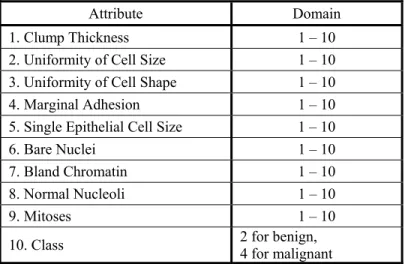
Table 1. Wisconsin Breast Cancer Attributes Name and Data Type
Attribute Domain 1. Clump Thickness 1 – 10
2. Uniformity of Cell Size 1 – 10 3. Uniformity of Cell Shape 1 – 10 4. Marginal Adhesion 1 – 10 5. Single Epithelial Cell Size 1 – 10
6. Bare Nuclei 1 – 10
7. Bland Chromatin 1 – 10 8. Normal Nucleoli 1 – 10
9. Mitoses 1 – 10
10. Class 2 for benign, 4 for malignant
Using a MATLAB random number generator, 30 data sets are selected from entire data set. And then, separate benign and malignant data sets are used to calculate the MS. Nineteen data sets are benign and eleven data sets are malignant. The healthy (benign) data sets are generalized. The correlation matrix and inverse correlation matrix are calculated. Finally, the Mahalanobis Distances for the selected data sets are calculated as shown in Table 3. The correlation matrix, standard deviation and mean of the healthy data sets are used for the MD of the entire 683 data sets. Figure 1 shows the general procedure of MD calculation.
Figure 1. General MTS Process
Table 2. Selected Wisconsin Breast Cancer Data and Mahalanobis Distance
Attribute
A B C D E F G H I Class MD 1 5 1 1 3 4 1 3 2 1 2 1.754 2 5 1 2 10 4 5 2 1 1 2 1.608 3 1 1 1 1 2 1 2 1 1 2 0.572 4 1 1 1 1 2 5 1 1 1 2 1.635 5 5 1 1 6 3 1 1 1 1 2 0.847 6 5 1 1 1 2 1 2 2 1 2 0.844 7 3 1 1 1 2 1 3 1 1 2 0.395 8 4 1 2 1 2 1 3 1 1 2 0.444 9 5 1 1 1 2 1 1 1 1 2 0.47 10 5 1 1 1 2 2 2 1 1 2 0.383 11 4 1 3 3 2 1 1 1 1 2 0.941 12 5 2 2 2 2 1 1 1 2 2 1.895 13 3 1 1 3 2 1 1 1 1 2 0.436 14 5 1 3 1 2 1 2 1 1 2 0.888 15 5 1 1 1 2 1 2 2 1 2 0.844 16 1 1 1 2 2 1 3 1 1 2 0.855 17 1 3 1 1 2 1 2 2 1 2 1.681 18 4 2 1 1 2 2 3 1 1 2 1.039 19 5 1 1 1 2 1 1 1 1 2 0.47 20 10 10 8 10 6 5 10 3 1 4 75.8 21 10 10 10 7 9 10 7 10 10 4 333 22 7 9 4 10 10 3 5 3 3 4 71.82 23 5 10 10 8 5 5 7 10 1 4 119.5 24 5 5 5 2 5 10 4 3 1 4 28.76 25 8 6 5 4 3 10 6 1 1 4 33.5 26 8 4 4 1 2 9 3 3 1 4 19.76 27 4 2 3 5 3 8 7 6 1 4 43.02 28 6 1 3 1 4 5 5 10 1 4 85.88 29 10 4 7 2 2 8 6 1 1 4 28.15 30 9 5 8 1 2 3 2 1 5 4 43.34
WBC Data from USC
Randomly Selected Data
Mahalanobis Distance Mahalanobis
Space
Calculate Accuracy
Adjust Threshold
Table 2 shows the attribute data and calculated Mahalanobis Distance. In the case of the normal (healthy) data sets, the MD value is very small and the average of MD is close to one. The abnormal MD values are larger than normal which illustrates the classification ability of MD. Figure 2 represents the MD of the normal and abnormal data.
0 50 100 150 200 250 300 350
1 2 3 4 5 6 7 8 9 10 11 12 13 14 15 16 17 18 19 20 21 22 23 24 25 26 27 28 29 30
MD
Mahalanobis Distance of Normal and Abnormal
normal
abnormal
Figure 2. Normal and Abnormal MD
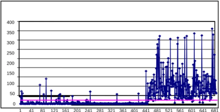
With the previous results, the selected data can classify the normal and abnormal case. Next, all of the data sets are tested with the previously obtained MS. The correlation coefficient matrix, mean and standard deviation of normal data are used for the test. The threshold value can be adjusted for the purpose of minimizing error. The accuracy of this simulation is 95.9%. Only 30 data sets out of the 683 data sets available were used for constructing the MS. The test accuracy is high compared to size of sample data.
Figure 3. Wisconsin Breast Cancer Test Results
Finally, using OA and SN ratio, the significance of each attribute is tested. With an L12 orthogonal array, the levels of each row decide whether that attribute is included or excluded. Since the L12 orthogonal array has 12 rows, eight different cases exist and the Mahalanobis space of each case is calculated. Abnormal test data is used for calculating the SN ratio. Since the deviation of the abnormal case is bigger than the normal case, the difference between using some attributes and excluding attributes can be easily detected. Table 3 represents the L12 orthogonal array and SN ratio.
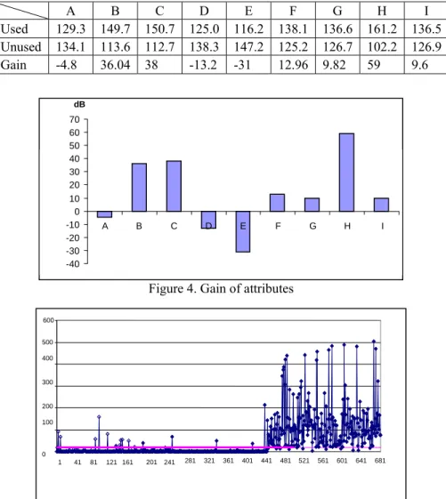
Table 4 and Figure 4 show the optimization results. The negative gained attributes do not affect the system much and can be neglected for the next process. The attributes B, C, F, G, H and I are selected and used to construct another MS and calculate MD. Figure 5 shows the classification results. With only 6 attributes used for this test, the accuracy of classification is 95.6%.
0 50 100 150 200 250 300 350 400
Table 3. L12 Orthogonal Array and SN Ratio A B C D E F G H I S/N ratio 1 1 1 1 1 1 1 1 1 1 1 1 31.6 2 1 1 1 1 1 2 2 2 2 2 2 16.45 3 1 1 2 2 2 1 1 1 2 2 2 31.12 4 1 2 1 2 2 1 2 2 1 1 2 20.11 5 1 2 2 1 2 2 1 2 1 2 1 13.9 6 1 2 2 2 1 2 2 1 2 1 1 16.07 7 2 1 2 2 1 1 2 2 1 2 1 18.27 8 2 1 2 1 2 2 2 1 1 1 2 26.05 9 2 1 1 2 2 2 1 2 2 1 1 26.18 10 2 2 2 1 1 1 1 2 2 1 2 7.24 11 2 2 1 2 1 2 1 1 1 2 2 26.52 12 2 2 1 1 2 1 2 1 2 2 1 29.79
Table 4. Level Average SN Ratio and Gain
Figure 4. Gain of attributes
Figure 5. Optimization results (6 attributes)
A B C D E F G H I Used 129.3 149.7 150.7 125.0 116.2 138.1 136.6 161.2 136.5 Unused 134.1 113.6 112.7 138.3 147.2 125.2 126.7 102.2 126.9 Gain -4.8 36.04 38 -13.2 -31 12.96 9.82 59 9.6
-40 -30 -20 -10 0 10 20 30 40 50 60 70
A B C D E F G H I
dB
0 100 200 300 400 500 600
5.2 Comparison study with feed forward neural network
Back propagation neural network was used for predicting breast cancer. Certain amounts of the test samples, such as 20, 30, 50 and 100 data sets, were randomly selected and tested to compare the ability of both MD and neural network. The MATLAB back propagation neural network algorithm was used for this test. For training, certain amounts of data were used for validation testing. The neural network was designed with an input layer, and one hidden layer and output layer. The number of input nodes is the same as the number of attributes, and the number of output node is always one. Generally, the total number of nodes are about half of training data.
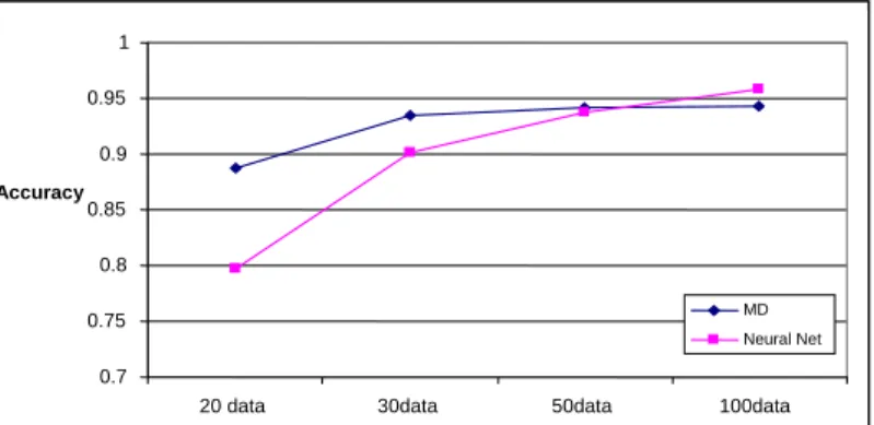
Table 5 represents the classification accuracy of Mahalanobis Distance associated with different data sizes (from 20 to 100). With the same data size, 10 replications were conducted. Table 6 represents accuracy test results with the neural network. Finally, Figure 6 shows the comparison of the average classification accuracy for MTS and NN associated with different data sizes.
Table 5. Accuracy of Mahalanobis Test Results with Various Data Sizes
data20 data30 data50 data100 1 0.946 0.936 0.925 0.962 2 0.846 0.955 0.962 0.961 3 0.928 0.933 0.958 0.909 4 0.911 0.949 0.946 0.949 5 0.838 0.946 0.934 0.950 6 0.794 0.896 0.929 0.924 7 0.880 0.956 0.953 0.936 8 0.895 0.941 0.920 0.933 9 0.918 0.915 0.949 0.947 10 0.920 0.921 0.944 0.959 MD 0.887 0.935 0.942 0.943
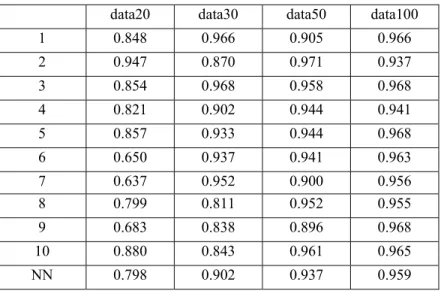
Table 6. Accuracy of Neural Network Test Results with Various Data Sizes
data20 data30 data50 data100 1 0.848 0.966 0.905 0.966 2 0.947 0.870 0.971 0.937 3 0.854 0.968 0.958 0.968 4 0.821 0.902 0.944 0.941 5 0.857 0.933 0.944 0.968 6 0.650 0.937 0.941 0.963 7 0.637 0.952 0.900 0.956 8 0.799 0.811 0.952 0.955 9 0.683 0.838 0.896 0.968 10 0.880 0.843 0.961 0.965 NN 0.798 0.902 0.937 0.959
Figure 6. Comparison of the Average Classification Accuracy for Neural Network and MTS
6. CONCLUSION
The main idea of Dr. Taguchi’s quality engineering is analyzing a complicated and time consuming system with efficiency. In multivariate systems, the existence of multi-collinearity (incidences of strong correlations) makes it difficult to analyze the system. But in most cases, there is a tradeoff between time and effort to analyzing a system. In this study, for diagnosis breast cancer, we can remove three attributes without significantly degrading diagnosis accuracy.
Neural networks require some amount of data and time for training. The comparison study with back propagation neural network illustrated that in case of small data sizes the MTS has better performance and better yet, unlike NN, requires no training time.
However, there are some problems that need to be addressed. In MTS, it is very important to select a “normal” or “healthy” group before constructing the MS. Classification largely depends on the normal samples. Determination of the threshold value and the application for multiple class cases are areas for further study.
REFERENCES
[1]
Asada M. (2001), Wafer yield prediction by the Mahalanobis-Taguchi system, IEEE International Workshop on Statistical Methodology 6; 25-28.[2]
Hassoun M.H. (1995), Fundamentals of artificial neural networks, Cambridge, MA, MIT Press.[3]
Hayashi S., Tanaka Y., Kodama E. (2001), A new manufacturing control system using Mahalanobis distance for maximizing productivity; IEEE Transactions 15(4); 59-62.[4] Jain Anil K., Duin Robert P.W., Mao Jianchang (2000), Statistical pattern recognition: A review, IEEE Transaction on Pattern Analysis and Machine Intelligence 22(1); 4-37.
[5] Jugulum R., Monplaisir L. (2002), Comparison between Mahalanobis-Taguchi- system and artificial neural networks, Journal of Quality Engineering Society, 10(1); 60-73.
[6] Jugulum R., Taguchi G., Taguchi S., Wilkins J. (2003), Discussion of A review and analysis of Mahalanobis-Taguchi System, Technometrics 45(1); 16-21
.
0.7 0.75 0.8 0.85 0.9 0.95 1
20 data 30data 50data 100data
Accuracy
MD Neural Net
[7] Lande U., Mahalanobis distance: A theoretical and practical approach;
http://biologi.uio.no/fellesavdelinger/finse/spatialstats/Mahalanobis%20distance.ppt (2003). [8] Taguchi G., Chowdury S., Wu Y. (2001), The Mahalanobis Taguchi system, McGraw Hill, New York. [9] Taguchi, G., Jugulum R. (2000), New trends in multivariate diagnosis; Indian Journal of Statistics, 62,
Series B; 233-248.
[10] Taguchi G., Jugulum R. (2002), The Mahalanobis-Taguchi strategy: A pattern technology system, John Wiley & Sons.
[11] Taguchi S. (2000), Mahalanobis Taguchi system, Proceedings of ASI Taguchi Symposium, Detroit, MI.
[12] Woodall W. H., Koulelik R., Tsui K. L., Kim S. B., Stoumbos Z. G., Carvounis C. P. (2003), A review and analysis of the Mahalanobis Taguchi, Technometrics, 45(1); 1-30.
[13] Wolberg W. H., Wisconsin breast cancer database;
http://www.uwplatt.edu/csse/Courses/cs303/as/data/cancer.html January 8, (1991).
[14] Wu, Y. (2004), Pattern Recognition Using Mahalanobis Distance, Journal of Quality Engineering