BONE DENSITY MEASUREMENT VIA RADIOGRAPHIC CALIBRATION
A Thesis presented to
the Faculty of California Polytechnic State University, San Luis Obispo
In Partial Fulfillment
of the Requirements for the Degree
Master of Science in Agriculture, with Specialization in Animal Science
by
ii © 2010
iii COMMITTEE MEMBERSHIP
TITLE: Bone Density Measurement via Radiographic Calibration
AUTHOR: Amber Jean Bowen
DATE SUBMITTED: May 2010
COMMITTEE CHAIR: Matthew A. Burd, D.V.M, M.S.
COMMITTEE MEMBER: John Craig, Ph.D.
COMMITTEE MEMBER: Ronald Brown, Ph.D.
iv ABSTRACT
Bone Density Measurement via Radiographic Calibration Amber Jean Bowen
Musculoskeletal injuries are the most common injuries sustained by athletes and military recruits and can result in decreased performance and lifelong disability. So common and costly are these injuries that the American Academy of Orthopedic Surgeons has provided guidelines for future research, including recommendations for the development of a large animal model of bone injury (USDA 2001). In human and veterinary medicine, digital radiography represents the primary diagnostic tool the physician uses to diagnose skeletal injury. Advances in digital radiography have provided the veterinarian with opportunities to make both simple and complex radiographic assessments. We investigated a simple quantitative measurement of the solar, concave aspect of the distal phalanx in the horse, termed the Palmar-Metric (PM). The PM was a significant predictor of solar cup volume (p < 0.001) and negatively correlated with age (r2 = 0.28, p < 0.05) as determined from 544 radiographs of the distal phalanx from the left and right front feet. Therefore, veterinarians should be aware of the age related change in the solar, concave aspect of the distal phalanx in the horse.
v varying radiographic exposure intensity (kV) and exposure time (mAs), Al BDI was a significant predictor of bone BDI (r2 = 0.960, p < 0.001) and bone OD (r2 = 0.971, p < 0.001). This method of calibration can be utilized by the radiologist to accurately assess bone OD regardless of technique, and allow direct comparison of radiographs taken under different exposure settings. This method successfully quantifies bone OD via measurement of BDI from standardized digital radiographs, allowing for the opacity of radiographs to be truly comparable when taken under different circumstances.
vi ACKNOWLEDGMENTS
I would like to express my sincere appreciation to Dr. Matthew Burd for his willingness to accept me as a graduate student, his continual challenging of me to achieve even more than I believed I could, and his unwillingness to accept anything less from me than what he believed I was capable of doing. I would also like to thank him for his continual support and guidance in my aspirations for veterinary school, which I couldn’t have achieved without him.
I would like to thank Dr. John Craig and Monique Craig for all their support and never ending stream of new ideas. Thank you, John, for working with me every step of the way, I couldn’t have done it without your remarkable insight and programming skills. Thank you and EponaTech, Inc. for coaching me in new techniques for research in the fields of radiology and biomechanics.
I would like to express my gratitude to Dr. Brooke Humphrey for agreeing to serve on my committee at the last minute.
vii TABLE OF CONTENTS
Page
LIST OF TABLES ... ix
LIST OF FIGURES ... x
I. LITERATURE REVIEW ... 1
1.1 Basics of Radiology ... 1
1.2 Applications of Radiology ... 6
1.3 Determination of Bone Quality ... 9
1.4 Standardization of Digital Radiographs ... 13
1.5 Justification for Work ... 15
II. INTRODUCTION ... 18
III. SIMPLE RADIOGRAPHIC STANDARDIZATION ... 20
3.1 Materials and Methods ... 20
3.2 PM Quantification ... 20
3.3 Standardization of the PM ... 20
3.4 PM and Age ... 27
3.5 PM Precision ... 27
3.6 Statistical Analysis ... 30
3.7 Results... 30
IV. COMPLEX RADIOGRAPHIC STANDARDIZATION ... 39
4.1 Materials and Methods ... 39
4.2 Determining BDI ... 39
4.3 Radiographic Method ... 39
4.4 BDI at Varying Radiographic Exposures ... 40
viii
4.6 Quantification of Optical Bone Density ... 46
4.7 Error Associated with Optical Bone Density ... 53
4.8 Statistical Analysis ... 57
4.9 Results ... 57
V. DISCUSSION ... 80
ix LIST OF TABLES
Table Page
1. Mean PM by age for 325 horses of various breeds ... 33
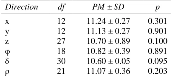
2. Mean PM with varying radiograph position ... 37
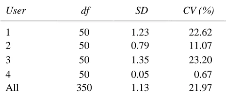
3. PM user precision error ... 38
4. BDI of Al wedge and bone with varying exposures ... 61
5. BDI accuracy with Al step-wedge ... 62
6. BDI of cortical bone step-wedge ... 65
7. Correction coefficient for bone OD ... 69
8. OD LM rotational error ... 74
9. OD DP rotational error... 75
10. OD with and without soft tissue and bone marrow... 76
11. OD soft tissue and bone marrow error ... 78
x LIST OF FIGURES
Figure Page
1. X-ray transmission diagram ... 2
2. Film versus digital dynamic range ... 4
3. Structure of a typical long bone ... 10
4. PM determination... 19
5. LM radiograph of third phalanx cadaver bone ... 21
6. PM determination from a cadaver third phalanx bone ... 24
7. Solar cup volume determination ... 25
8. Lateral toe length and height determination ... 26
9. Standard LM radiograph of the distal limb of the horse ... 26
10. Radiographic rotational and positional errors ... 29
11. PM versus solar cup volume regression... 31
12. PM versus lateral toe length and height regression ... 32
13. PM for left and right front feet by age. ... 35
14. PM versus age regression ... 36
15. DP positioning of third metacarpal cadaver bone ... 41
16. Regions of interest for bone and Al wedge ... 43
17. Al wedge and Al step-wedge radiograph ... 44
18. Standard curve from Al wedge ... 45
19. Regions of interest for Al wedge and Al step-wedge ... 48
20. Known mass attenuation coefficients by kV ... 49
21. Bone wedge radiograph ... 51
22. Regions of interest for bone wedge ... 53
23. Regions of interest and limb diameter for density determination ... 54
24. Region of interest while varying radiographic positioning... 56
xi
26. Bone BDI versus Al BDI at varying exposures ... 59
27. Al step-wedge standardization of BDI ... 60
28. Bone step-wedge BDI versus areal bone density regression ... 61
29. Al BDI versus Al areal density ... 65
30. Al BDI versus Al areal density regression ... 66
31. Correction coefficient regression ... 67
32. OD with and without soft tissue and bone marrow ... 71
1
I. LITERATURE REVIEW
1.1. Basics of Radiology
Radiography is a widely used diagnostic technique in veterinary medicine. According to the Behr-Lambert law, a radiographic image is produced when energy from an X-ray source is transmitted through a patient and detected by a sensor (Figure 1). The X-ray source or tube is a diode tube made of Pyrex glass that encloses a vacuum. A modern X-ray tube contains a heated filament (cathode) that releases X-rays which are accelerated across high voltage produced by electrodes onto a target (anode). X-rays are produced as the accelerated electrons interact with the target, emerging in all directions to be restricted by collimators. In this manner, an incident X-ray beam is produced (Hendee and Ritenour 2002).
2 Figure 1. X-ray transmission from the source is detected by the sensor along the horizontal axis (x) is dependent on density, thickness (t) and absorption coefficient of the sample.
x
t
source
3 in evaluation of chest (Garmer et al. 2000, Fink et al. 2002, Hirsch et al. 2001), pulmonary (MacMahon et al. 1986) and skeletal (Zahringer et al. 2001, Strotzer et al. 1995) abnormalities.
Additionally, DR provides a wide dynamic range while traditional X-ray film is somewhat limited due to silver halide crystals. The wide dynamic range found in DR is due to the large dynamic range of the digital receptors, meaning that there is a wider functional range of receptor exposure. When using X-ray film outside of the limited dynamic range the film easily becomes over or under exposed. This is not a problem in DR as the image is less likely to be over or under exposed at relatively low or high exposures (Figure 2) (Sprawls 1987, Garmer et al. 2000).
Similar to film radiography, an image is produced in DR when energy is transmitted through a patient and detected by a sensor; the measured difference in transmission is displayed as a digital image. Each data point acquired is a transmission measurement through the patient along a given line between the source and the sensor’s detector pixel (Figure 1). The transmitted radiation detected by each pixel is converted to an electrical signal and displayed on a computer screen as a greyscale, with brighter pixels detecting less transmitted radiation (Curry et al. 1990).
4 Figure 2. From Sprawls 1987, film radiography (A) has a limited dynamic range due to the silver halide in film that is easily over or under exposed at receptor exposure extremes. Digital radiography (B) provides a wide dynamic range due to the response of digital receptors to a wider range of exposures.
5 the external electronics where the signal is digitized and stored. The most commonly used sensing element is composed of an amorphous silicon (a-Si) photodiode layer (Beutel et al. 2000).
6 1.2. Applications of Radiology
Radiology is the most commonly used technique to assess bone quality by subjective evaluation for bone fractures, pathology, or any change from normality in bone size, shape and ossification. Radiology is used for a wide array of diagnoses, including detection of osteoporosis (Szulc 2006), cancer (Hirsch et al. 2001) and stress fractures in soldiers and athletes (Pentecost et al. 1964, Krause and Thompson 1943). DR represents the primary diagnostic tool the physician uses to diagnose skeletal injury.
In horses, the most common application of DR is in evaluation of the cause of lameness, the most important origin of loss of use for the horse (Lindner and Dingerkus 1993). Musculoskeletal injuries account for the majority of racing and training deaths in both Thoroughbreds and Quarter Horses (Johnson 1993, Estberg et al. 1993, 1996, Palmar 1986). In performance horses, fractures not due to a specific traumatic event occur often, and are considered to be fatigue or stress fractures. Pre-existing stress fractures are often seen in severe pelvic, scapular, humeral and tibial fractures (Stover et al. 1991, 1993, Johnson 1993, Johnson et al. 1994). Microfractures and stress fractures can be caused by normal physiological strain if stress is repetitive or applied in a different plane than normal, or by physiological strain beyond the normal limits (Nielsen et al. 1997). In 1990, Frost theorized that if enough micro-damage occurs cortical bone remodeling will be triggered. Despite many studies that have been conducted to determine risk factors associated with stress fractures in performance horses, even today, there exists relatively little insight into the prevention of these performance related injuries.
7 modeling when overloaded (Jones et al. 1977, Goodship et al. 1979, Woo et al. 1981, Bloomfield 1995, Lanyon 1984, Meade et al. 1984, Rubin and Lanyon 1984, 1985, Burr et al. 1989). Remodeling due to increased strain occurs via increased deposition of bone on the periosteal surface (Goodship et al. 1979) and also by decreased resorption of bone from the endosteal surface (Jones et al. 1977, Woo et al. 1981). Bones that are under-loaded are remodeled to decrease the amount of bone present such as occurs in astronauts during space flight (Cavolina et al. 1997), cases of disuse (Lanyon 1984, Rubin and Lanyon 1984, 1985, Skerry and Lanyon 1995, Thomas et al. 1996) and during deconditioning (Porr et al. 1998).
9 1.3. Determination of Bone Characteristics
The structural unit of compact bone is called the osteon or Haversian system. Each osteon is an elongated cylinder oriented along the long axis of the bone which group together to form lamella. Collagen fibers in a lamella are able to withstand mechanical stress and attribute to bone strength. Collagen and other organic material makes up 1/3 of the matrix, and contribute to the structure, flexibility and tensile strength of bone. The inorganic components consist of hydroxyapatites the majority which is calcium phosphate. Hydroxyapatites account for bone hardness and are the major contributors to bone density (Ensminger 1994).
A typical long bone consists of a cortex or a dense outer layer and an inner medulla. A long bone has a shaft or a diaphysis in the middle region and each end is expanded into a region termed the epiphysis. The diaphysis consists of cortical or compact bone containing the Haversian system and a hollow middle called the medullary cavity which is filled with marrow. The epiphyses are composed largely of trabecular or spongy bone. At the diaphysis, there is cortical bone surrounding bone marrow, and very little associated soft tissue (Figure 3).
11 More advanced techniques including quantitative ultrasound, computed tomography and MRI aid in assessing bone modalities such as stiffness (Moris et al. 1995), 3D bone structure and micro-architecture (Feldkamp et al. 1989), change in bone geometry due to exercise (Daly et al. 2004), and BMD (Chappard et al. 1997). However, these methods are limiting as the clinician can only make a subjective appraisal of bone quality and comparison of images is difficult when taken with different techniques such as exposure setting, focal distance and equipment, or taken overtime.
True bone density can be measured by determination of bone weight and volume. Compact bone has a measured density of 1.85 g/cm3, accurate to the µg/cm3. Trabecular bone density ranges from 0.2 to 0.6 g/cm3 while soft tissue has the same density as water at 1.00 g/cm3 (Berger et al. 2000). However, it is unpractical to use this method to measure bone density in vivo and alternate techniques have been developed that are good indicators of bone density. Ex vivo, studies report an increase in bone ash weight (g/cc) or percent bone mineralization during periods of bone growth (Hammett 1925), and decrease with increased age (Leichter et al. 1981, Riggs et al. 1981). Weaver and Chalmers 1966 and Bell et al. 1967 demonstrated a significant correlation between compressive strength and ash weight. However, the use of ash weight as a significant predictor for bone density and strength may be affected by the method of bone preservation, drying, and testing techniques (Sedlin 1965, Sedlin and Hirsch 1966, Walmsley 1953).
13 1.4. Calibration of Digital Radiographs
To make accurate dimensional and complex measurements, the method of medical imaging needs to be calibrated. With the frequency and ease of use with DR, radiography is an ideal method for digital imaging standardization. For the veterinarian, DR offers a compact, portable method to evaluate bone quality. As bone characteristics and opacification is often subjectively compared to assess bone structure abnormalities and pathology, quantitative assessment of various aspects of bone morphology via radiography would be extremely valuable.
Many methods have successfully generated basic dimensional measurements from a radiograph by scaling the image to an object of known size, allowing for reproducible radiographic measurements equivalent to actual size (Kummer et al. 2004, Rocha et al. 2004, White et al. 2008). This is accomplished by insertion of a marker of known dimensions into the radiograph in plane with the patient, affording quantitative analysis of many variables such as bone displacement, vascular canal diameter, and bone thickness (Linford et al. 1993, Craig et al. 2001, Rocha et al. 2004, Raub et al. 1989). Standardized radiographic measurements have been shown to aid in morphometric analyses of the distal limb of the horse, including changes in bone size due to injury and remodeling (Raub et al. 1989), third phalanx positioning due to laminitis (Parks and O’Grady 2003) and hoof trimming (Kummer et al. 2006).
14 radiography, an aluminum (Al) wedge of increasing thickness and uniform density is commonly included in a radiographic study as a comparison for OD, affording determination of bone OD in terms of mm Al or radiographic bone Al equivalents (Meakim et al. 1981, Inoue et al. 2006, Kolbeck et al. 1999). This method is most readily applied in a research setting as each radiograph must be taken with exactly the same technique (exposure setting and focal distance). Additionally, OD is measured at regions of interest as determined by the researcher. With this system OD cannot quantitatively be compared between studies due to varying radiographic techniques.
15 1.5. Justification for Work
Despite the many studies that have been conducted to determine risk factors associated with stress fractures in athletes and soldiers, there exists relatively little insight into the prevention of these performance related injuries (Myburgh et al. 1990, Giladi et al. 1985). Musculoskeletal injuries occur in 50% of soldiers in Iraq and Afghanistan and the military spends over 1.5 billion dollars annually treating and managing these injuries (USDA 2001). So common and costly are these injuries that the American Academy of Orthopedic Surgeons has provided guidelines for future research. Fundamental aspects of these recommendations include the development of a large animal model of bone injury (Pollak and Calhoun 2006). Using common digital radiography, quantitative measurements of bone quality would be valuable in a wide range of applications in the medical, military and veterinary fields by evaluation of bone integrity, fracture risk and results of performance training (Heggie et al. 2001). DR is commonly used to detect fractures in large animals and the third metacarpal bone of the horse represents an ideal model of bone fracture due to the high frequency of performance related injury. This will allow assessment of variables that indicate stress fracture risk in vivo, utilizing currently existing and practical technology.
16 the standard technology used to diagnose osteoporosis in humans by determination of BMD at specific sites such as the second metacarpal bone, lateral spine or the femoral neck (Szulc 2006). BMD is considered low in each of these sites when compared to a national average, however, as DEXA is not standardized, BMD is dependent on the site scanned and not completely comparable between DEXA machines (Tabensky et al. 1996). Further, comparison of BMD scans to population average BMD for specific sites is not available or practical to the veterinary clinician. Unlike DEXA, DR has the advantage for veterinary clinicians of being extremely portable, relatively inexpensive, and practical in a field setting. Despite the many methods used today to evaluate bone morphology, none are used at near the frequency as DR in qualifying fractures. DR provides the clinician with portable rapid image acquisition, diagnosis, and images that can easily be stored or transferred for off-site review. However, due to the lack of standardization of digital radiographic images, an image cannot entirely be compared to another taken under different conditions such as exposure settings, positioning, and equipment. Development of a quantitative measurement for radiographic bone density using standard radiographs will be valuable to the veterinarian in assessing bone integrity, fracture risk and results of performance training (Heggie et al. 2001).
17 wedge standard, but none are practical in a non-research, clinical setting. Some authors have attempted to eliminate the confounding factor of bone size by measurement of limb circumference (Raub et al. 1989), however, there are no methods available that allow calibration for quantification of OD with different DR systems and exposure settings (Nagamine et al. 2000).
18
II. INTRODUCTION
In the first study, a novel morphometric measurement was generated to evaluate the volume of the solar aspect of the distal phalanx in the horse via radiography. Recent advances in standardized digital radiology and software development have supported accurate, quantitative, measurements of the equine digit. Furthermore, these measurements may improve treatment of distal limb lameness by providing the veterinarian with quantitative radiographic assessments of the equine digit (Rocha et al. 2004, Kummer et al. 2004, Hunt 2002, Parks and O’Grady 2003). Our objectives were to describe a novel measurement of the solar, concave aspect of the distal phalanx, termed the Palmar-Metric (PM), via simple radiographic calibration and demonstrate the manner in which the PM changes with age.
The second study contained three parts. In the first part, a quantitative measurement for radiographic bone density was developed that accurately evaluates the radiographic opacity of bone, termed the brightness/darkness index (BDI), under different exposure conditions. This method will be valuable to the veterinarian in assessing bone integrity, fracture risk and results of performance training when using a common digital radiography system (Heggie et al. 2001). By creating a standardized curve for the BDI of the bone as determined from the BDI along an Al wedge standard, and characterizing BDI as a smooth, continuous function dependent on intensity and exposure time, we can account for changes in radiographic density due to changes in exposure, affording brightness calibration of any radiograph.
20
III. SIMPLE RADIOGRAPHIC CALIBRATION
3.1. Materials and Methods
This is one of two studies presented examining standardized digital radiographic measurements of the distal limb of the horse. This study concentrated on a novel radiographic volumetric measurement of the concave, solar aspect of the distal phalanx, termed the PM, and examined how the PM correlated with age in the horse.
3.2. PM Quantification
A method to determine the PM from any standard lateral medial (LM) radiograph was developed to evaluate the solar concavity of the distal phalanx. From a digital radiograph, a line we term the palmar curve was traced from the tip of the distal phalanx along the most palmar aspect of the radio-dense line to the proximal palmar aspect of the articular margin of the distal phalanx (Figure 4A,B). The PM was calculated by creating a coordinate system within the radiograph based on the palmar curve and position of the distal phalanx (Figure 4C). A reference rectangle was then constructed and the area within the rectangle defined above and below the palmar curve. The PM was expressed as a percentage of the area under the palmar curve relative to the area of the reference rectangle (Figure 4D).
3.3. Calibration of the PM
22 markers of known length to scale the image. High quality digital LM radiographs were taken of the 65 cadaver bones and hoof block (Figure 5). The PM was determined using the method described above (Figure 6). Radiographs were taken at 65 kV, 0.06 seconds and 15 mA with a focal distance of 26 inches.
For each bone, physical volume of the solar concavity was measured using modeling putty by filling the solar aspect of the distal phalanx. The distal phalanx with putty was pressed onto a hoof block and excess putty was removed. The putty was cut lateral to medial at the position of the orthogonal projection of the extensor process when viewed from above (Figure 7A). The putty dorsal to this cut was removed and discarded. The remaining putty was removed and its volume was measured via water displacement (Figure 7B,C).
Additionally, third phalanx lateral toe length and lateral height were determined from digital radiographs of the 65 cadaver bones (Figure 8). Lateral height was determined as the length perpendicular to the most palmar aspect of the solar surface and intersecting the most proximal point of the extensor process. Toe length was measured from the palmar tip of lateral height to the tip of the third phalanx. Lateral toe length and height were evaluated to determine if they were significant predictors for solar cup volume.
25 Figure 7. The solar cup volume of the distal phalanx was measured using modeling putty. The putty was cut lateral to medial at the position of the orthogonal projection of the extensor process when viewed from proximal to distal (A). The putty dorsal to this cut was removed and discarded. The remaining putty was removed (B) and its volume (cc) was measured via water displacement (C).
A
B
27 3.4. PM and Age
Subsequently, three independent users determined the PM from 544 high quality LM digital radiographs of the front feet of horses (Figure 9). Radiographs were taken with the inclusion of a standardized hoof block, and were obtained from various
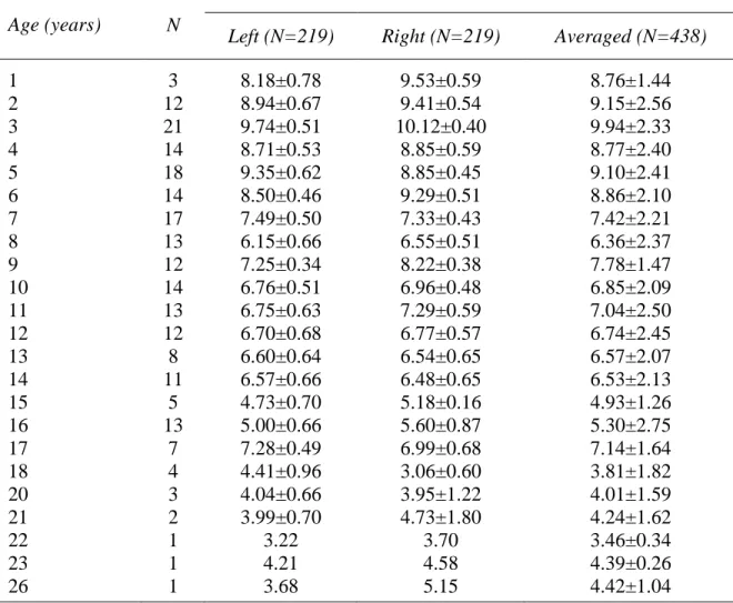
veterinary clinics and farms for horses of known age and breed. Of the 544 radiographs, 438 (219 pairs) were right and left front feet pairs, resulting in a total of 325 horses radiographed. The average age of the 325 horses was 8.8 ± 5.1 years.
Radiographs were taken with various digital systems, at unknown exposure and focal distance, depending on the veterinarian’s discretion. Digital images were imported into the software program Metron-DVM (EponaTech).
3.5. PM Precision
29 Figure 10. Coordinates for radiographic rotational and positional errors, with angle φ
representing a rotation about the x-axis, angle δ representing a rotation about the y-axis, and angle θ representing a rotation about the z-axis. The digital sensor plate was positioned in the y,z-plane.
x
δ
φ
z
30 3.6. Statistical Analysis
Linear regression was used to assess the relationship between PM and solar cup volume for the 65 cadaver bones. Of the 544 LM radiographs, 219 left and right pairs were analyzed for differences between left and right PM versus age by comparing slopes using a two sample paired t-test. Linear correlation was used to assess the relationship of age, lateral height, toe length and radiographic positioning on PM. All statistical tests were performed using Minitab and were based on a 2-sided null hypothesis of no difference and a level of significance set at 0.05.
3.7. Results
Calibration of the PM was performed via determination of solar cup volume and PM for 65 distal phalanx cadaver bones. Solar cup volume is shown to be a statistically significant predictor of the PM (t(63) = 26.64, p < 0.001, Figure 11). Furthermore, 91.9 % of the variability in the PM is explained by the regression relationship between PM and solar cup volume (r2 = 0.9185). PM increases as lateral height increases (r2 = 0.668, t(63) = 11.07, p < 0.001) and toe length increases (r2 = 0.684, t(63) = 11.483, p < 0.001). Both lateral height and toe length are significant predictors of PM, however, less variability is explained with height or toe length (Figure 12).
31 Figure 11. Experimentally measured solar cup volume versus PM, determined from standard lateral medial radiographs of 65 distal phalanx cadaver bones (t(63) = 24.32, p < 0.001, r2 = 0.918).
y = 0.939x + 0.717 R² = 0.918
0 5 10 15 20
0 5 10 15 20
P
M
(
%
)
32 Figure 12. PM versus third phalanx lateral height (top) and toe length (bottom), determined from lateral medial radiographs of 65 third phalanx cadaver bones (p < 0.001)
y = 19.69x - 17.62 R² = 0.668
0 5 10 15 20
0.5 1 1.5 2
P
M
(
%
)
Lateral Height (inches)
y = 19.81x - 13.07 R² = 0.684
0 5 10 15 20
0.5 1 1.5 2
P
M
(
%
)
33 Age (years)
Mean Palmar-Metric ± SD (%) N
Left (N=219) Right (N=219) Averaged (N=438)
1 3 8.18±0.78 9.53±0.59 8.76±1.44
2 12 8.94±0.67 9.41±0.54 9.15±2.56
3 21 9.74±0.51 10.12±0.40 9.94±2.33
4 14 8.71±0.53 8.85±0.59 8.77±2.40
5 18 9.35±0.62 8.85±0.45 9.10±2.41
6 14 8.50±0.46 9.29±0.51 8.86±2.10
7 17 7.49±0.50 7.33±0.43 7.42±2.21
8 13 6.15±0.66 6.55±0.51 6.36±2.37
9 12 7.25±0.34 8.22±0.38 7.78±1.47
10 14 6.76±0.51 6.96±0.48 6.85±2.09
11 13 6.75±0.63 7.29±0.59 7.04±2.50
12 12 6.70±0.68 6.77±0.57 6.74±2.45
13 8 6.60±0.64 6.54±0.65 6.57±2.07
14 11 6.57±0.66 6.48±0.65 6.53±2.13
15 5 4.73±0.70 5.18±0.16 4.93±1.26
16 13 5.00±0.66 5.60±0.87 5.30±2.75
17 7 7.28±0.49 6.99±0.68 7.14±1.64
18 4 4.41±0.96 3.06±0.60 3.81±1.82
20 3 4.04±0.66 3.95±1.22 4.01±1.59
21 2 3.99±0.70 4.73±1.80 4.24±1.62
22 1 3.22 3.70 3.46±0.34
23 1 4.21 4.58 4.39±0.26
26 1 3.68 5.15 4.42±1.04
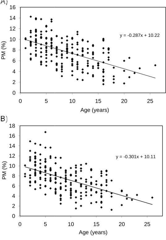
34 regression lines for PM and age for left (-0.27 ± 0.03 % per year) and right (-0.29 ± 0.03 % per year) front feet were not significantly different from each other (t(217) = -0.676, p = 0.75, Figure 13). The PM for left and right front feet was averaged to obtain one PM value for each horse. There was strong evidence that the age of the horse was a significant predictor for PM, and decreased at a rate of 0.28 ± 0.02 % per year (r2 = 0.33, t(217) = -10.4, p < 0.001, Figure 14).
Figure 13. PM versus age
t(217) = -9.85, p < 0.001) front regression lines do not differ
0 2 4 6 8 10 12 14 16 0 5 P M ( % ) 0 2 4 6 8 10 12 14 16 18 0 5 P M ( % )
versus age for 219 left (A, t(217) = -9.78, p < 0.001) and 219 right (B, 0.001) front feet of various breed horses. The slopes of the two
differ significantly (t(217) = -0.676, p = 0.75).
y = -0.287x + 10.22
10 15 20 25
Age (years)
y = -0.301x + 10.11
10 15 20 25
Age (years)
36 Figure 14. Average PM (top) and PM (bottom) versus age for 219 horses of various breeds. PM decreased at a rate of 0.294 % per year (t(217) = -10.4, p < 0.001).
0 2 4 6 8 10 12
0 5 10 15 20 25
A v e ra g e P M ( % ) Age (years)
y = -0.294x + 10.17
0 2 4 6 8 10 12 14 16
0 5 10 15 20 25
37
Direction df PM ± SD p
x 12 11.24 ± 0.27 0.301
y 12 11.13 ± 0.27 0.901
z 27 10.70 ± 0.89 0.100
φ 18 10.82 ± 0.39 0.891
δ 30 10.60 ± 0.05 0.095
ρ 21 11.07 ± 0.36 0.203
38
User df SD CV (%)
1 50 1.23 22.62
2 50 0.79 11.07
3 50 1.35 23.20
4 50 0.05 0.67
All 350 1.13 21.97
39
IV. Complex Radiographic Calibration
4.1. Materials and Methods
This is the second study examining standardized radiographic measurements in the distal limb of the horse. This study contained three parts: the first part concentrated on calibration of BDI in the third metacarpal of the horse over different exposure ranges, the second part concentrated on measurement of bone OD via digital radiographs, and the third part concentrated on error associated with the measurement of bone OD due to effects of soft tissue, radiographic positioning and user error.
4.2. Determining BDI
BDI was evaluated in the same manner in all instances. First, digital radiographs were imported into the software program Metron-DVM (EponaTech). To determine BDI a unit-less value was assigned to each 16 bit pixel on a greyscale from 0 to 65,535, with zero being completely black and 65,000 being completely white. A predetermined area or region of interest was generated by forming a rectangle using the software program Metron-DVM. The BDI for the area is determined by averaging the greyscale value of each pixel in the area, using Excel (Microsoft). In determining BDI pixels with BDI equal to the BDI of the background were not included.
4.3. Radiographic Method
40 2.70 g/cm3. The Auto-Scaler contained metal markers that standardized the dimensions of the radiograph when imported into Metron. All radiographs were taken with a portable X-ray system (Min X-X-ray HF80 or HF100+) and X-X-ray sensor (Canon CXDI 60G, Vetel Diagnostics).
4.4. BDI at Varying Radiographic Exposures
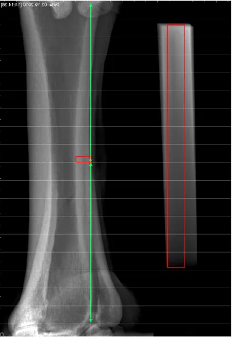
As the BDI of a region of interest decreases with increasing X-ray exposure, the nature of this effect on both cortical bone and an Al standard needed to be evaluated to correctly assess cortical bone BDI at varying radiographic exposure settings. A third metacarpal equine cadaver bone was placed on a wooden block with Al wedge and Auto-Scaler. The cadaver bone was positioned perpendicular to the ground in the center of the line of exposure with the Al wedge and Auto-Scaler positioned on either side. The bone was placed to produce a standard dorsal palmar (DP) radiograph (Figure 15). The focal distance was 26 inches, with the plane of interest containing the cadaver bone, Al wedge, and Auto-Scaler positioned against the face of the sensor. Radiographs were taken at all available combinations of pre-set exposure intensities ranging from 55 to 80 kV with 5 kV intervals, and exposure times from 0.02 to 0.14 seconds every 0.02 seconds. All radiographs were taken at 15 mA, the only setting available for the X-ray source.
41 Figure 15. Dorsal palmar positioning of a third metacarpal equine cadaver bone on a wooden block with Auto-Scaler (left) of known dimensions and Al wedge (right) of known thickness and density. The nutrient foramen (red arrow) can be seen as a dark spot on the diaphysis.
42 equal to the diameter of the nutrient foramen (NF) (Figure 16). The NF was used as a marker so that the measurement of bone BDI was always for the same region of interest to ensure that changes in BDI were solely due to effects of radiographic exposure. Al BDI and bone BDI were evaluated for dependency on exposure intensity and exposure time. Al BDI was compared to bone BDI for each combination of X-ray intensities and exposure times to ensure Al BDI correlated linearly with that of bone. We expect a smooth linear correlation of bone BDI to Al BDI over a range of exposures to ensure that X-rays interact the same with Al and bone, and that the interaction was some function of exposure that was easily standardized. This allowed for BDI calibration of radiographs taken at varying exposure intensity and exposure time using an Al wedge standard.
4.5. Calibration of BDI
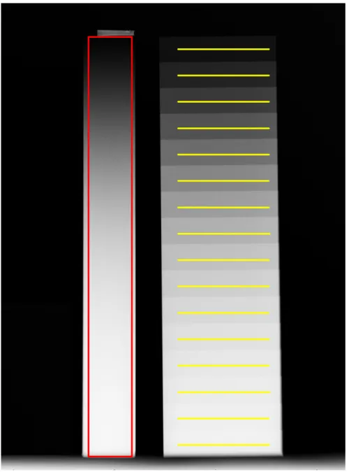
44 Figure 17. Standard curve of BDI versus thickness of Al (mm Al) for a radiograph of an Al wedge taken at 60 kV, 0.06 seconds and 15 mA.
0 10000 20000 30000 40000 50000 60000 70000
0 5 10 15 20
B
D
I
46 Radiographs were taken in combinations from 40 to 90 kV and 0.04 to 0.08 seconds at a focal distance of 26 inches. Radiographs were standardized using the Al wedge standard curve. The thickness of each step of the Al step-wedge was measured with 6 inch digital calipers (Fisher Scientific) with 0.01 mm accuracy. Additionally, step thickness was measured from a standardized radiograph in terms of mm Al. A marker was placed at the end of the Al wedge to ensure the full length was used to create an accurate standard curve. The step thickness was measured using a region of interest that was centered horizontally on the step and 9 pixels wide (Figure 19). The region of interest excluded the edges of the step where BDI was most likely to fluctuate due to edge affects.
4.6. Quantification of Optical Density
Measurement of BDI or mm Al is generally only used for research as its value is dependent on the grayscale chosen by the individual and the attenuation properties of the material being measured. OD is preferred to BDI as an indicator of bone mineral density as confirmed by DEXA, and is commonly used in human medicine (Nagamine et al. 2000). In determining OD, the Beer-Lambert law applies to all photo-film techniques:
, (1)
Where transmitted beam intensity, incident beam intensity,
linear attenuation coeficient, and thickness of the material (Curry et al. 1990).
The equation can be rewritten as:
⁄ ,
where !
47
48 coefficient is dependent upon attenuation of an X-ray through matter, and is affected by several different mechanisms such as energy of the incident X-rays, the attenuator’s atomic mass number, Rayleigh or coherent scattering, Compton or incoherent scattering, photoelectric absorption, and electron/positron pair production. The value of the mass attenuation coefficient is independent of the density of the attenuator (Curry et al. 1990). In medically relevant exposure ranges of 50 to 90 kV, the effects of coherent scatter and pair production are relatively insignificant as the average atomic numbers of cortical bone (13.7) and Al (13) are low (Graham and Cloke 1982, Hubbell and Seltzer 2004). Although the mass attenuation coefficients vary significantly over this range, the mass attenuation coefficient ratio is relatively constant at 0.886 ± 0.026 (Figure 20) (Hubbell and Seltzer 2004).
Radiographic density or OD, commonly referred to as luminosity or opacity of the bone sampled, is defined as:
"# $%& '
'( )!* (2)
And OD of Al, for example, would be:
"#+, )-!*.+,
Comparing optical densities of Al and bone, we set "#+,equal to "#/: -!*.+, -!*./
*/ -!+,⁄!/. · -+,⁄ . · */ +, (3)
49 Figure 20. Mass attenuation coefficients for cortical bone (blue) and Al (red). The mass attenuation coefficient ratio (green) is relatively constant at 0.886 ± 0.026 (Hubbell and Seltzer 2004). 0 0.5 1 1.5 2 2.5 3 3.5 4 4.5
0 20 40 60 80 100 120 140 160
M a ss A tt e n ti o n C o e e fi ci e n t (μm )
X-Ray Energy (kV)
μm Bone
μm Al
50 bone density, which is proportional to OD. For example, two materials such as bone and Al of known density and thickness are radiographed. The point at which the radiograph exhibits equal BDI for both materials, the mass attenuation ratio for the materials can be calculated using Equation 3 (Carricart-Ganivet and Barnes 2007, Chalker et al. 1985). By determining the mass attenuation coefficient ratio for cortical bone and Al using an Al wedge of known areal density, bone density can be quantified from a standardized digital radiograph.
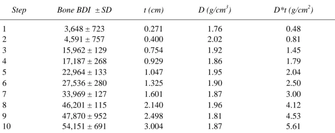
In determining the mass attenuation coefficient ratio, a cortical bone step-wedge was created of known density and increasing thickness. Cortical bone was obtained from a third metacarpal equine cadaver bone in the mid-diaphysis region. The cortical bone was cut into slices using a diamond blade tile saw. The average dimension of each slice was 15.28 ± 3.3 mm square and 4.23 ± 1.0 mm thick. A bone step-wedge was created by stacking each bone slice in increasing thickness from the one slice up to 6 slices thick, consecutively from Row 1 to Row 10. Scotch tape was used on the sides of the bone slices to hold them in place, forming a total of ten steps of increasing thickness. The thickness and volume corresponding with each bone step was determined using 6 inch digital calipers (Fisher Scientific) with 0.01 mm accuracy. Weight was measured using a digital balance (Accu-224, Fisher Scientific) with 0.1 mg accuracy. The density for each bone step was determined by dividing weight by volume for each step. Slices were stored at 5 °C and kept hydrated in a saline solution.
52 with the Al wedge on one side. BDI was determined for each step of bone and for the standard curve obtained from the Al wedge (Figure 22). Standardized curves were created for bone BDI versus bone areal density, and Al BDI versus Al areal density. Where Al BDI was equal to bone BDI, the correlation between bone and Al areal density could be determined, and therefore the mass attenuation coefficient ratio. Radiographs were taken with a focal distance of 26 inches, with the plane of interest containing the bone wedge and the Al wedge positioned against the face of the sensor. Radiographs were taken at 60 kV, 15 mA and 0.08 seconds.
To test if bone OD was an accurate predictor of bone areal density for any exposure, further evaluation of the bone step-wedge was performed while varying kV. Radiographs were obtained of the bone step-wedge and Al wedge using methods described in the previous experiment. Radiographs were taken from 40 to 90 kV, 0.06 seconds and 15 mA at a focal distance of 26 inches. Bone OD was measured and compared to the areal density for each cortical bone step.
4.7. Error Associated with Optical Bone Density
54 Figure 23. Selection of 10 regions of interest (white lines) along a third metacarpal cadaver bone without soft tissue and bone marrow from a dorsal palmar (A) and lateral medial radiograph (B). The diameter of the bone was measured at each region of interest for both views. Both images contain an Auto-Scaler (left) and Al wedge (right).
55 scraping out the medullary cavity with a metal spoon. For all radiographs, bone OD was measured at 10 different regions of interest spaced equally proximal to distal along the midline of the third metacarpal (Figure 23). Each region of interest was equal to the diameter of the bone in width, and 9 pixels in height. Bone OD was analyzed for differences in each region of interest dependent on radiographic view (DP and LM) and presence of soft tissue and bone marrow. Additionally, the diameter of the third metacarpal bone at each of the regions of interest was measured on both LM and DP views to determine bone density. Bone density was determined by dividing OD from one view by the diameter measured from the opposite view for each region of interest. Radiographs were taken with a focal distance of 26 inches and exposure settings of 65 kV, 0.06 seconds and 15 mA.
Error in bone OD due to radiographic positioning was further investigated in a single region of interest at the mid-diaphysis of a third metacarpal cadaver limb. The region of interest was limited to a known area of cortical bone on the lateral wall in a DP view (Figure 24). Bone OD was determined for this region while varying the angle between the X-ray source and limb in two rotational planes: one proximal to distal and the second lateral to medial. Angles varied from 5 - 32 degrees proximal to distal, and from 10 - 30 degrees lateral to medial, with 0 degrees being normal. Radiographs were taken 66 kV, 0.06 seconds and 15 mA with a focal distance of 26 inches.
Figure 24. Selection of region (left) positioned at the mid
bone, determined from a dorsal palmar radiograph taken at
mA. The X-ray source was placed at 30 degrees rotation from a standard view.
regions of interest (red) for the Al wedge (right) and cortical bone at the mid-diaphysis in the lateral cortical region of the third metacarpal
from a dorsal palmar radiograph taken at 60 kV, 0.06 seconds ray source was placed at 30 degrees rotation from a standard
57 4.8. Statistical Analysis
Regression analyses were performed using the least squares method. Slope of the regression lines were shown to be different from zero determined by a Student’s t-test. Multi-variable analysis was done for BDI versus exposure intensity and time using an ANOVA and associated F-test. All statistical tests were performed using Minitab and were based on a 2-sided null hypothesis of no difference and a level of significance set at 0.05.
4.9. Results
While standardizing BDI, bone BDI decreased with increasing exposure intensity and exposure time. From 0.02 to 0.14 seconds and 55 to 80 kV, bone BDI ranges from 13,747 to 49,851 (Table 4A). Similarly, Al BDI decreased with increasing exposure intensity and exposure time, ranging from 21,388 to 54,328 (Table 4B). BDI correlated linearly with exposure intensity and exposure time for Al (r2 = 0.8594, F(2,39) = 119.2, p < 0.001) and bone (r2 = 0.9126, F(2,39) = 203.7, p < 0.001) (Figure 25). For each combination of intensity and exposure time, Al BDI showed a linear correlation with bone BDI (r2 = 0.9599, F(1,40) = 957.3, p < 0.001). As Al BDI increased per unit, there was an increase in bone BDI of 1.12 ± 0.04 (Figure 26).
58 Figure 25. BDI versus exposure intensity (top) and exposure time (bottom) determined from a dorsal palmar radiograph of a third metacarpal cadaver bone and Al wedge taken at varying exposure (p < 0.001).
0 10000 20000 30000 40000 50000 60000
50 55 60 65 70 75 80 85
B
D
I
Exposure Intensity (kV)
Bone Al 0 10000 20000 30000 40000 50000 60000
0 0.02 0.04 0.06 0.08 0.1 0.12 0.14 0.16
B
D
I
Exposure Time (sec)
Bone
59 Figure 26. Linear correlation of BDI of a third metacarpal cadaver bone versus Al BDI at varying exposure intensities (55-80 kV) and exposure times (0.02-.014 s) (p < 0.001).
y = 1.1225x - 12973 R² = 0.9599
0 10000 20000 30000 40000 50000 60000
20000 30000 40000 50000 60000
B
o
n
e
B
D
I
60 Figure 27. Regression of mm Al measured from a radiograph versus thickness of Al determined with calipers for 16 steps of an Al step-wedge. Greater variance is seen at steps thicker than 12 mm (p < 0.001).
y = 0.9846x - 0.2172 R² = 0.9922
0 5 10 15 20 25 30
0 5 10 15 20 25 30
61 Table 4. BDI at the nutrient foramen (A) and Al wedge (B) determined from a dorsal palmar radiograph of a third metacarpal at varying exposure intensities (55 – 80 kV) and exposure times (0.02 – 0.14 seconds).
A) Exposure Time (sec)
0.02 0.04 0.06 0.08 0.1 0.12 0.14
Int ens it y (k V )
55 49851.20 47324.93 48851.92 47979.78 45745.73 41531.48 39134.09 60 45854.03 48001.42 44886.04 40580.10 38567.94 33940.24 30970.81 65 45657.83 45258.55 46563.14 35112.90 31168.28 27543.62 25046.51 70 47970.69 39823.54 38583.39 29976.86 25877.64 23134.80 22218.42 75 43981.89 38335.79 31419.15 25567.06 22194.23 19800.11 18432.86 80 43221.42 36932.82 27441.96 22277.3 19188.45 16605.65 13747.36
B) Exposure Time (sec)
0.02 0.04 0.06 0.08 0.1 0.12 0.14
Int ens it y (k V )
62 Table 5. Thickness of Al (mm Al), average thickness of Al with standard deviation (Average ± SD), and actual thickness (t) of Al determined for 16 steps of an Al step-wedge. Thickness in mm Al was measured from digital radiographs taken from 50 to 90 kV at 0.06 seconds while actual thickness (Actual t) was measured using digital calipers. Percent error compared actual thickness of the step to radiographic quantification of average mm Al.
Step
mm Al at Varying kV
Actual t (mm) % Error 50 60 70 80 90 Average ± SD
1 1.90 1.91 1.99 2.01 2.14 1.99 ± 0.10 1.62 22.9
2 3.58 3.52 3.59 3.61 3.77 3.61 ± 0.09 3.20 12.9
3 5.16 5.07 5.15 5.15 5.28 5.16 ± 0.08 4.80 7.6
4 6.79 6.68 6.73 6.73 6.88 6.76 ± 0.08 6.40 5.6
5 8.39 8.27 8.28 8.28 8.42 8.33 ± 0.07 7.95 4.7
6 10.04 9.90 9.87 9.85 9.99 9.93 ± 0.08 9.60 3.4
63 wedge thickness as the regression slope was not significantly different than 1 (t(249) = 1.373, p = 0.171). At thicker steps of Al (steps 10 – 16) larger variation in mm Al was seen.
To determine OD for cortical bone, the relationship between OD and BDI was quantified. Bone BDI was shown to increase linearly with increasing areal bone density and therefore bone OD (r2 = 0.9716, F(1,1193) = 40,850, p < 0.001, Figure 28). From Row 1 to Row 10 of the bone wedge, the BDI ranged from 3,648 ± 723 to 54,151 ± 691 (Table 6). Similarly, Al BDI increased with increasing Al areal density and, therefore, Al OD, ranging from a BDI of 0 to 53,810 with a constant density of 2.70 g/cm3. Al thickness increased linearly along the length of the Al wedge from 0 to 4.26 cm before the slope of the standard curve began to decrease resulting in a nonlinear correlation with Al OD above 4.26 cm Al thick (Figure 29). For thicknesses under 4.26 cm Al a linear approximation could be made, allowing determination of the mass attenuation coefficient ratio from a single variant (r2 = 0.9973, F(1,631) = 232,800, p < 0.001, Figure 30). In addition, the ratio of the mass attenuation coefficients could be solved for by comparing Al OD to that of bone when Al BDI equals bone BDI, utilizing Equation 3. The mass attenuation coefficient ratio -!+,⁄!/. was estimated using regression equations from Figures 27 and 29. At the point where BDI was equal for both materials !+,⁄!/ was
determined to be 0.9042 (p < 0.001) (Appendix A). This allowed for determination of bone OD in terms of g/cm2.
64 Figure 28. Bone BDI determined from a radiograph of the bone step-wedge versus bone areal density measured with digital scale and calipers (p < 0.001).
y = 10460.53x - 28.70 R² = 0.9716
0 10000 20000 30000 40000 50000 60000 70000
0 1 2 3 4 5 6
B
o
n
e
B
D
I
65 Figure 29. Al BDI versus Al areal density for the length of the Al wedge. With areal density greater than 4 g/cm2 there is a visible decrease in slope of the standard curve.
0 10000 20000 30000 40000 50000 60000
0 2 4 6 8 10
A
l
B
D
I
66 Figure 30. Al BDI versus Al areal density determined for the linear region (0 – 40,000 BDI) of the Al wedge standard curve from a radiograph taken at 66 kV, 0.08 seconds and 15 mA (p < 0.001).
y = 9,482.03x + 1,078.49 R² = 0.9973
0 10000 20000 30000 40000 50000
0 1 2 3 4 5
A
l
B
D
I
67 Figure 31. Regression of areal bone density versus bone OD determined from radiographs of a cortical bone wedge at 40 to 90 kV.
y = 0.7414x + 0.5603 R² = 0.9907
0 1 2 3 4 5 6 7
0 1 2 3 4 5 6 7 8
B o n e A re a l D e n si ty ( g /c m 2)
68
Step Bone BDI ± SD t (cm) D (g/cm3) D*t (g/cm2)
1 3,648 ± 723 0.271 1.76 0.48
2 4,591 ± 757 0.400 2.02 0.81
3 15,962 ± 129 0.754 1.92 1.45
4 17,187 ± 268 0.929 1.86 1.79
5 22,964 ± 133 1.047 1.95 2.04
6 27,536 ± 280 1.325 1.90 2.50
7 33,969 ± 127 1.601 1.87 3.00
8 46,201 ± 115 2.140 1.96 4.12
9 47,870 ± 952 2.498 1.81 4.53
10 54,151 ± 691 3.004 1.87 5.61
69 Appendix A
Equation 3:
*// -!+,⁄!/. · *+,+, -!+,⁄!/. *//⁄*+,+,
Regression equations:
1#234 0.105 · *//) 0.023 1#+, 0.095 · *+,+,< 0.108
Solving for !+,⁄!/:
70 radiographs taken from 40 to 90 kV, resulting in a 0.741 increase in areal density per unit increase in bone OD (r2 = 0.9907, F(1,89) = 184.7, p < 0.001, Figure 31). Using the regression equation from Figure 31, bone areal density can be determined using the predictor variable bone OD accurate greater than 93% for exposure intensities of 50 – 90 kV (Table 7).
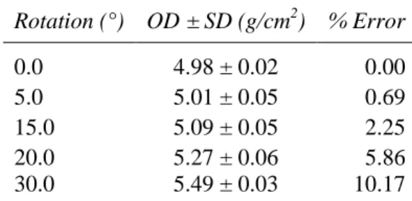
In measuring OD, errors associated with effects of radiographic positioning were evaluated. To assess error in OD due to positioning, bone OD was measured in the cortical region of the mid-diaphysis of a third metacarpal cadaver limb. At zero degrees lateral to medial rotation, OD was determined to be 5.70 ± 0.02 g/cm2. From 10 - 30 degrees of rotation in the lateral to medial direction average OD was 5.33 ± 0.24 g/cm2. Error in OD was greater than 10% with lateral to medial rotation greater than 18 degrees, and less than 3% with rotation under 5 degrees (Table 8). From 5 - 32 degrees of rotation in the proximal to distal direction the average OD was 5.17 ± 0.20 g/cm2, measured on a slightly different region of cortical bone as part of the third metacarpal was cut off the radiograph. Error in OD was less than 10% with proximal to distal rotation under 30 degrees, and less than 3% with rotation under 5 degrees (Table 9).
71 Figure 32. Bone OD versus 10 regions of interest (slice #) of known thickness determined from a dorsal palmar (A) and lateral medial (B) radiograph of a third metacarpal cadaver limb (A) and LM view (B). Bone OD was measured with soft tissue and marrow (blue), after the removal of soft tissue (red) and after the removal of soft tissue and marrow (green). 0 1 2 3 4 5
0 2 4 6 8 10 12
B o n e O D ( g /c m 2)
DP Slice #
A)
All No Tissue No Tissue/Marrow 0 1 2 3 4 50 2 4 6 8 10 12
B o n e O D ( g /c m 2)
LM Slice #
B)
All
No Tissue
72 Figure 33. Bone density versus 10 regions of interest (slice #) of known thickness determined from a dorsal palmar (A) and lateral medial (B) radiograph of a third metacarpal cadaver limb (A) and LM view (B). Bone density was measured with soft tissue and marrow (blue), after the removal of soft tissue (red) and after the removal of soft tissue and marrow (green).
0 0.2 0.4 0.6 0.8 1
0 2 4 6 8 10
D e n si ty ( g /c m 3 )
DP Slice #
A)
All No Tissue No Tissue/Marrow 0 0.2 0.4 0.6 0.8 10 2 4 6 8 10
D e n si ty ( g /c m 3)
LM Slice #
B)
All No Tissue
73
Step Average Bone OD ± SD D*t (g/cm2) % Error
2 0.84 ± 0.08 0.808 4.3
3 1.44 ± 0.08 1.445 0.1
4 1.65 ± 0.07 1.729 4.3
5 2.02 ± 0.04 2.040 1.2
6 2.46 ± 0.02 2.514 2.0
7 2.89 ± 0.05 2.999 3.6
8 3.93 ± 0.10 4.189 6.2
9 4.29 ± 0.12 4.530 5.2
10 5.73 ± 0.22 5.606 2.2
74
Rotation (°) OD ± SD (g/cm2) % Error
0.0 5.70 ± 0.02 0.00
10.0 5.55 ± 0.07 2.66
15.0 5.29 ± 0.02 7.16
18.0 5.27 ± 0.07 7.49
22.0 5.10 ± 0.09 10.60
29.0 5.08 ± 0.08 10.87
75
Rotation (°) OD ± SD (g/cm2) % Error
0.0 4.98 ± 0.02 0.00
5.0 5.01 ± 0.05 0.69
15.0 5.09 ± 0.05 2.25
20.0 5.27 ± 0.06 5.86
30.0 5.49 ± 0.03 10.17
76 A)
Slice
All No Soft Tissue No Soft Tissue or Marrow
OD
(g/cm2) t (mm) D (g/cm3)
OD (g/cm2)
t (mm)
D (g/cm3)
OD (g/cm2)
t (mm)
D (g/cm3)
1 2.33 4.30 0.28 1.69 3.31 0.56 1.63 3.31 0.55
2 2.56 4.54 0.29 1.89 3.42 0.61 1.84 3.42 0.59
3 2.70 4.48 0.31 2.10 3.62 0.64 2.03 3.62 0.62
4 2.75 4.35 0.34 2.25 3.70 0.67 2.20 3.70 0.66
5 3.02 4.54 0.37 2.37 3.86 0.68 2.39 3.86 0.69
6 3.23 5.17 0.38 2.53 4.00 0.70 2.60 4.00 0.72
7 3.47 5.25 0.40 2.76 4.28 0.71 2.80 4.28 0.72
8 3.88 5.86 0.45 3.00 4.56 0.73 3.11 4.56 0.75
9 4.30 7.31 0.49 3.16 4.87 0.72 3.31 4.87 0.75
10 4.56 7.10 0.60 3.47 5.39 0.71 3.64 5.39 0.75
B)
Slice
All No Soft Tissue No Soft Tissue or Marrow
OD (g/cm2)
t (mm)
D (g/cm3)
OD (g/cm2)
t (mm)
D (g/cm3)
OD (g/cm2)
t (mm)
D (g/cm3)
1 2.36 9.46 0.60 2.30 4.15 0.61 2.25 4.15 0.60
2 2.37 8.91 0.62 2.49 4.08 0.67 2.46 4.08 0.67
3 2.48 8.83 0.67 2.55 4.00 0.71 2.47 4.00 0.68
4 2.57 8.32 0.70 2.70 4.04 0.74 2.54 4.04 0.70
5 2.70 8.07 0.74 2.84 4.05 0.77 2.54 4.05 0.69
6 2.52 7.39 0.69 2.66 3.95 0.75 2.54 3.95 0.71
7 2.67 7.43 0.73 2.64 4.00 0.73 2.53 4.00 0.70
8 2.64 6.44 0.73 2.66 3.92 0.75 2.50 3.92 0.70
9 2.39 5.35 0.65 2.51 3.96 0.70 2.42 3.96 0.67
10 2.61 4.79 0.71 2.58 4.09 0.70 2.49 4.09 0.67
77 regression lines for OD and bone density associated with no soft tissue and no marrow were not significantly different from each other in both the LM and DP views (p > 0.05). The slopes of the regression lines for OD associated with soft tissue were significantly different from the other conditions of no soft tissue and no soft tissue and marrow, but only in the DP view (p < 0.001, Table 11). The slopes of the regression lines for bone density associated with soft tissue were significantly different from the other conditions of no soft tissue and no soft tissue and marrow, but only in the LM view (p < 0.001, Table 11).
78
Sample OD ± SD (g/cm
2
) Density ± SD (g/cm3)
LM DP LM DP
All 2.53 ± 0.13* 3.28 ± 0.76 0.39 ± 0.10 0.68 ± 0.05†
No Soft Tissue 2.59 ± 0.15* 2.52 ± 0.57* 0.67 ± 0.05† 0.71 ± 0.05†
No Soft Tissue/Marrow 2.47 ± 0.09* 2.55 ± 0.66* 0.68 ± 0.07† 0.68 ± 0.03†
*,†
no significant difference between values (P > 0.05)
79
User df SD CV (%)
1 40 0.10 3.28
2 40 0.13 4.01
3 40 0.05 1.51
All 280 0.11 3.46
80
V. DISCUSSION
81 Because the PM is a ratio, it is not dependent on size of the distal phalanx and can be assessed independent of breed related differences in foot size. The PM ranged from 1.24 – 16.74% and was shown to be negatively correlated with age (Figures 13, 14). Therefore, young horses have a significantly greater PM than older horses in this study. Additionally, the PM for left and right front feet were not significantly different at any age class in our study (t(217) = -0.676, p = 0.75, Figure 13). Measurement of the PM may afford the veterinarian a quantitative technique to assess the presence of significant unilateral foot pathology that would result in differences between the left and right PM for an individual horse. As the age-related, gradual demineralization of bones is a well studied phenomenon, especially in osteoporosis in humans, we believe that in horses the decreased depth of the solar concavity over time is due to gradual demineralization of the third phalanx along the solar margin. Because the distal phalanx is so variable in morphology, especially along the solar margin, it is not an ideal model for radiographic determination of osteoporotic changes.
82 developed a method based on standardized digital radiographs that affords the veterinary professional accurate and repeatable measurement of areal bone density.
83 In determining bone OD, a bone step-wedge of known density and thickness was created (Table 6). BDI was shown to be a significant predictor of areal density in both Al (r2 = 0.9973, F(1,631) = 232,800, p < 0.001, Figure 30) and bone (r2 = 0.9716, F(1,1193) = 40,850, p < 0.001, Figure 28). Further, our goal was to determine bone OD in terms of g/cm2 with known values for the mass attenuation coefficient ratio, density and thickness of Al. The ratio of the mass attenuation coefficients was solved for by comparing Al OD to that of bone when Al BDI equals bone BDI, utilizing Equation 3. The mass attenuation coefficient ratio -!+,⁄!/. was estimated using regression equations from Figures 27
and 29. At the point where BDI was equal for both materials, !+,⁄!/ was determined
84 using the regression equation, bone areal density could be determined from a radiograph with less than a 7 % error (Table 7). This method permits accurate evaluation of BDI and, therefore, bone OD independent of the exposure setting.
85 11). We observed that the presence of both soft tissue and bone marrow significantly affected the measurement of OD when measuring from the DP view. OD measured from the DP view of an intact limb was significantly greater than for the LM view or for any other condition. This is explained by our method of determining OD as an average value for a given region of interest, meaning OD was much greater when the soft tissue was compacted into a smaller region of interest in the DP view. From the LM view, the region of interest encompassed the bone only, and therefore much less soft tissue. From our results, there were no statistically significant effects of soft tissue on OD measurements from the LM view of an intact third metacarpal limb.
86 determining OD. Also, use of the third metacarpal diameter for the thickness value of cortical bone may be decreasing our value for bone density, as it is an overestimate of cortical bone thickness by including the thickness of soft tissue. Further, filtering techniques performed by the Canon software apply various complex and non-linear imaging processing algorithms to the image, which may be applied to a single pixel individually, to a pixel depending on neighboring pixels, or even to a pixel depending on non-localized effects from a different region of the image. Overall, determination of bone density from standardized radiographs is a complex task due to effects of soft tissue and the difficulty in determining cortical bone thickness.
Effects on OD determination due to radiographic positioning were also evaluated. We observed less than a 10% error in OD as long as the user did not exceed 18 degrees of lateral to medial rotation and 30 degrees of proximal to distal rotation (Table 8, 9). Error in OD measurement due to user error was also determined to be low, with a maximum CV of 4.01% (Table 12). Although error in the 5% range is not acceptable for accurate medical diagnosis of decreased bone mineralization in humans, this method allows quantitative comparison of OD from any digital radiograph standardized in this manner.