Server-based Inference of Internet Performance

Server-based Inference of Internet Performance

Microsoft Research Abstract—

We investigate the problem of inferring the packet loss characteristics of Internet links using server-based measure-ments. Unlike much of existing work on network tomog-raphy that is based on active probing, we make inferences based on passive observation of end-to-end client-server traf-fic. Our work on passive network tomography focuses on

identifying lossy links (i.e., the trouble spots in the network).

We have developed three techniques for this purpose based on Random Sampling, Linear Optimization, and Bayesian Inference using Gibbs Sampling, respectively. We evaluate the accuracy of these techniques using both simulations and Internet packet traces. We find that these techniques can identify most of the lossy links in the network with a man-ageable false positive rate. For instance, simulation results indicate that the Gibbs sampling technique has over 80% coverage with a false positive rate under 5%. Furthermore, this technique provides a confidence indicator on its infer-ence. In the case of Internet traces, validating the inferences is a challenging problem. We present a method for indirect validation, which suggests that the false positive rate is man-ageable.

I. INTRODUCTION

The Internet has grown rapidly in terms of size and het-erogeneity in recent years. The set of hosts, links, and net-works that comprise the Internet is diverse. This presents interesting challenges from the viewpoint of an Internet server, such as a Web site, whose goal is to provide the best possible service to its clients. A significant factor that the server must contend with is the dissimilar and change-able network performance experienced by clients.

The goal of our work is to investigate ways to infer the performance of the Internet by passively monitoring exist-ing network traffic between a server and its clients. Our goal is to go beyond characterizing end-to-end network performance by developing techniques to infer the perfor-mance of interior links in the network.

There are a number of ways in which the server could benefit from such characterization and inference. Infor-mation on the stability or predictability of network perfor-mance to one or more clients could be used to adapt con-tent for speedy delivery to the client(s) [19]. Information on bottlenecks or other hot spots within the network could be used to direct clients to replica servers so that they avoid the hot spot. Such information could also be used by a Web

site operator to have the hotspot problem resolved in coop-eration with the concerned ISP(s). The focus of this paper, however, is on the inference of network performance, not on its applications.

One question is what “network performance” means. Clearly, the performance metrics that matter depend on the application. Latency may be most critical in the case of game servers while throughput may be the most impor-tant metric for software download servers. In our study, we primarily focus on the packet loss rate because it is the most direct indicator of network congestion.1 We view the packet loss rate and RTT metrics as being more fundamen-tal than throughput since the latter is affected by factors such as the workload (e.g., bulk transfers versus short Web transfers) and the transport protocol (e.g., the specific vari-ant of TCP). Furthermore, it is possible to obtain a rough estimate of throughput knowing the packet loss rate and RTT, using an analytical model of TCP such as [14].

Here is an overview of the rest of this paper. In Section II, we discuss related work. In Section III, we present the key findings from our analysis of end-to-end packet loss rate based on traces gathered at the busy microsoft.com site. We find that packet loss rate correlates poorly with hop count, is stable for a period of several minutes, and exhibits a limited degree of spatial locality. These findings suggest that it would be interesting and feasible to try and identify the few lossy links, whether shared or non-shared, that dominate the end-to-end loss rate.

This sets the stage for our main focus, Passive Network Tomography, which we present in Section IV. The goal here is to identify the lossy links in the interior of the net-work by passively observing the end-to-end performance of existing traffic between a server and its clients. This is in contrast to the previous work on network tomogra-phy (e.g., [3]) that has been based on active probing. We develop three techniques for passive network tomography: Random Sampling, Linear Optimization, and Bayesian In-ference using Gibbs Sampling. In Section V, we evaluate these techniques using extensive simulations and find that we are able to identify more than 80% of the lossy links with a false positive rate under 5%. In Section VI, we also apply these techniques to the traffic traces gathered at the

1

We have also done some characterization of the round-trip time (RTT) metric, but we do not present those results in this paper.

microsoft.com site. Validation is challenging in this set-ting since we do not know the true loss rate of Internet links. We present a method for indirect validation, which suggests that the false positive rate is manageable.

Finally, we present our conclusions in Section VII.

II. RELATED WORK

There have been numerous studies of Internet perfor-mance. We can broadly classify these studies as either active or passive. Active studies involve measuring Inter-net performance by injecting traffic (in the form of pings, traceroutes, TCP connections, etc.) into the network. In contrast, passive studies analyze existing traffic obtained from server logs, packet sniffers, etc. Our study is a pas-sive one.

Several studies (e.g., [16], [21]) have examined the tem-poral stability of Internet performance metrics through ac-tive measurements. In [16] Paxson reports that observing (no) packet loss along a path is a good predictor that we will continue to observe (no) packet loss along the path. However, the magnitude of the packet loss rate is a lot less predictable. Zhang et. al. examines the stationarity of packet loss rate and available bandwidth [21]. They find that the correlation in the loss process mainly comes only from back-to-back loss episodes, and not from “nearby” losses. Throughput has a close coupling with the loss pro-cess, and can often be modeled as a stationary IID process for periods of hours.

Several studies have also examined similar issues by studying traces gathered passively using a packet sniffer. The authors in [2] used traces from the 1996 Olympic Games Web site to analyze the spatial and temporal sta-bility of TCP throughput. Using traceroute data, they con-structed a tree rooted at the server and extending out to the client hosts. Clients were clustered together based on how far apart they are in the tree. The authors report that clients within 2-4 tree-hops of each other tend to have sim-ilar probability distributions of TCP throughput. They also report that throughput to a client host tends to remain sta-ble (i.e., within a factor of 2) for time scales of many tens of minutes.

Packet-level traces have also been used to characterize other aspects of network traffic. In [1] Allman uses traces gathered at the NASA Glenn Research Center Web server to study issues such as TCP and HTTP option usage, RTT and packet size distributions, etc. Mogul et al. uses packet-level traces to study the effectiveness of delta compression for HTTP [12].

Our study is similar to [2] in that it is based on packet sniffer traces gathered passively at a busy server. However, our analysis is different in many ways. We focus on packet

loss rate rather than TCP throughput for the reasons men-tioned previously. More importantly, we go beyond simply characterizing the end-to-end loss rate by using this infor-mation to identify the lossy links in the network.

This last aspect of our work lies in the area of Network Tomography, which is concerned with the inference of the internal network characteristics based on end-to-end ob-servations. The observations can be made through ac-tive probing (either unicast or multicast probing) or pas-sive monitoring. MINC [3] and [17] base their inference on loss experienced by multicast probe packets while [4], [5] use closely-spaced unicast probe packets striped across multiple destinations. A common feature of the above techniques is that they are based on active injection of probe packets into the network. Such active probing im-poses an overhead on the network and runs the risk of al-tering the link characteristics, especially when applied on a large scale (e.g., on the path from a busy server to all of its clients).

In [18] and [10], the authors take a passive approach in detecting shared bottlenecks. The former requires senders to cooperate by time stamping the packets while the latter requires an observer that receives more than 20% of the output traffic of the bottleneck (i.e., light background traf-fic). Tsang et al. [20] estimate loss rate for each link by passively observing closely spaced packet-pairs. A prob-lem, however, is that existing traffic often may not contain enough such packet-pairs to make an inference. Further-more, their evaluation is based on very small topologies containing a dozen (simulated) nodes, and it is not clear how well their technique would scale to large topologies.

III. ANALYSIS OFEND-TO-ENDLOSSRATE

We analyzed the end-to-end loss rate information de-rived from traffic traces gathered at the microsoft.com site. Due to space limitations, we only present a sketch of our experimental methodology and our key findings here. The technical report version of this paper [15] includes a de-tailed description of our experimental setup and method-ology, and detailed results, including graphs.

The traces were gathered by running the tcpdump tool on a machine connected to the replication port of a Cisco Catalyst 6509 switch. The packet sniffer was thus able to listen on all communication between the servers connected to the same switch and their clients located anywhere in the Internet. We inferred packet loss based on TCP retransmis-sions, which is reasonable since TCP is conservative about retransmissions. We gathered multiple traces, each over 2 hours long and containing over 100 million packets.

The key findings of our analysis of end-to-end loss rate are that (a) the correlation between loss rate and hop count

is weak, regardless of whether hop count is quantified at the granularity of routers, autonomous systems, or address prefix clusters, which suggests that a few lossy links domi-nate the end-to-end loss rate; (b) loss rate tends to be stable over a period of several minutes (where stability refers to the notion of “operational stationarity” described in [21]); and (c) clients that are topologically close to each other experience more similar loss rate than clients picked at random, but in general there is only a limited degree of spatial locality in loss rate. These findings suggest that it would be interesting and feasible to try and identify the few lossy links, whether shared or non-shared, that dom-inate the end-to-end loss rate. This sets the stage for our work on passive network tomography, where we develop techniques to provide greater insight into some of these conjectures.

IV. PASSIVENETWORKTOMOGRAPHY

In this section, we attempt to identify lossy links in the network based on observations made at the server of end-to-end packet loss rates to different clients. As noted in Section II, much of the prior work on estimating the loss rate of network links has been based on the active injec-tion of probe packets into the network. In contrast, our goal here is to base the inference on passive observation of existing network traffic. We term this passive network tomography.

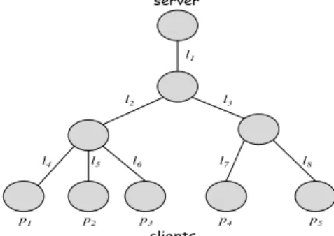
Figure 1 depicts the scenario of interest: a server trans-mitting data to a distributed set of clients. By passively observing the client-server traffic, we can determine the number of packets transmitted by the server to each client. Based on the feedback from the clients (e.g., TCP ACKs, RTCP receiver reports), we can also determine how many of those packets were lost in the network.

We assume that the network path from the server to each client is known. In the experiments reported in this paper, the path to each client was determined using the traceroute tool [9]. While these traceroutes do constitute active mea-surement, this need not be done very frequently or in real time. (Indeed previous studies have shown that end-to-end Internet paths generally tend to be stable for significant lengths of time. For instance, [22] indicates that very of-ten paths remain stable for at least a day.) Moreover, it may be possible determine the server-to-client path “pseudo-passively” by invoking the record route option (IPv4) or extension header (IPv6) for a small subset of the packets.

The set of paths from the server to its clients is likely to form a tree (as depicted in Figure 1) and so our ex-planations here are couched in terms of tree-specific ter-minology. However, we do recognize that the topology may not strictly be a tree (for instance, because of

tran-sient route fluctuations), so our techniques do not depend on the topology being a tree. We elaborate on this point in Section IV-B. l1 l8 l7 l6 l2 l4 l5 l3 p1 p2 p3 p4 p5

Fig. 1. A sample network topology as viewed from a server. The link loss rates are denoted byliand the end-to-end loss rate at the clients are denoted bypj.

A. Challenges

Identifying lossy links is challenging for the following reasons. First, network characteristics change over time. Without knowing the temporal variation of the network link performance, it is hard to correlate performance ob-served by different clients. Second, even when the loss rate of each link is constant, it may not be possible to definitively identify the loss rate of each link. Given M clients and N links, we have M constraints (corre-sponding to each server→client path) defined overN vari-ables (corresponding to the loss rate of the individual links). For each clientCj, there is a constraint of the form

1−Q_i∈Tj(1−li) = pj where Tj is the set of links on the path from the server to clientCj,li is the loss rate of linki, andpjis the end-to-end loss rate between the server and clientCj. There is not a unique solution to this set of constraints ifM < N, as is often the case.

To make the problem tractable, we make the simplify-ing assumption that the loss rate of each link is constant. Although this is not a very realistic assumption, it is a rea-sonable simplification in the sense that some links consis-tently tend to have high loss rates whereas other links con-sistently tend to have low loss rates. Zhang et al. [21] re-ported that the loss rate remains operationally stable on the time scale of several minutes. Our temporal locality anal-ysis based on microsoft.com traces also confirms it (Sec-tion III and [15]).

There is still the problem that we may not, in general, be able to determine a unique assignment of loss rate to network links. We address this issue in several ways.

First, we collapse a linear sections of a network path with no branches into a single virtual link2. This is appro-priate since it would be impossible to determine the loss

2

phys-rates of the constituent physical links of such a linear sec-tion using end-to-end measurements.

Second, although there may not be a unique assignment of loss rate to network links, two of our techniques seek a parsimonious explanation for the observed end-to-end loss rates. (This bias is implicit in the case of Random Sam-pling and explicit in the case of Linear Optimization.) So given a choice between an assignment of high loss rates to many links and an assignment of high loss rates to a small number of links, they would prefer the latter. The underly-ing assumption is that a lossy link is relatively uncommon. If most of the links are lossy, network tomography may not be very useful any way since there are not specific trouble spots to pinpoint. On the other hand, our Gibbs Sampling technique uses a uniform prior and so is unbiased.

Finally, we set our goal to primarily be the identification of links that are likely to have a high loss rate rather than inferring a specific loss rate for each link. We believe that the identification of the most lossy links in itself would be very useful for applications such as network diagnosis and server selection.

We now describe the three different techniques we have explored and developed for passive network tomography. We present these in roughly increasing order of sophisti-cation. However, as the experimental results in Section V indicate, even the simplest technique, yields good results. B. Random Sampling

The set of constraints mentioned in Section IV-A define a space of feasible solutions for the set of link loss rates. (We denote a specific solution aslL=

S

i∈Lli whereLis the set of all links in the topology.) The basic idea of ran-dom sampling is to repeatedly sample the solution space at random and make inferences based on the statistics of the sampled solutions. The solution space is sampled as follows. We first assign a loss rate of zero to each link of the tree (Figure 1). The loss rate of link iis bounded by the minimum (say lmin_i ) of the observed loss rate at the clients downstream of the link. We pick the loss rate, li, of the linkito be a random number between 0 andlmin_i . We define the residual loss rates of a client to be the loss rate that is not accounted for by the links whose loss rates have already been assigned. We update the residual loss rate of a clientCj to1−Q 1−pj

i∈T_j0(1−li)

whereT_j0 is the sub-set of links along the path from the server to the clientCj for which a loss rate has been assigned. Then we repeat the procedure to compute the loss rate at the next level of the tree by considering the residual loss rate of each client

ical links and virtual links.

in place of its original loss rate. At the end, we have one sample solution forlL.

We iterateR times to produce R random solutions for l_L. We draw conclusions based on the statistics of the in-dividual link loss rates,li, across theRrandom solutions. For instance, if the average loss rate assigned to a link across all samples is higher than a threshold, we conclude that the link is lossy.

Note that we compute a loss rate only for those clients to whom the server has transmitted at least a threshold num-ber of packets. Only this subset of the clients and the topol-ogy induced by them is considered in the random sampling algorithm.

The sampling procedure outlined above is biased be-cause the order in which links are picked matters. As we assign loss rates to an increasing number of links, the loss rate bound on the remaining links gets tighter. So links that are picked early in an iteration are likely to be as-signed a higher loss rate than ones picked later. Thus in the above algorithm, links higher up in the tree (i.e., close to the server), which are picked early in the process, tend to get assigned a higher loss rate. Of course, the loss rate bound on a link higher up in the tree might be tighter to begin with because of there is a greater chance that one or more downstream clients will have experienced a low loss rate.

This bias, however, has a positive side-effect in that it favors parsimonious solutions (i.e., ones in which the ob-served client loss rates can be accounted for by assigning a high loss rate to fewer links). If many clients are ex-periencing a high loss rate, an explanation that involves one shared, lossy link higher up in the tree is more plausi-ble than one that involves a large number of independently lossy links.

Note that our random sampling algorithm would work the same way even if the topology were not a tree. In fact, at any stage in an iteration, we can pick an arbitrary link, determine the bounds on its loss rate by examining all server→client paths that traverse the link, and then ran-domly assign it a loss rate. Just like in a tree topology, we could start by picking links close to the server and then working our way towards the clients.

The random sampling algorithm has the advantage of being simple. However, it is quite susceptible to estima-tion errors in the client loss rate. Due to a statistical vari-ation, a single client that is downstream of a true lossy link could experience a low loss rate. This would cause the random sampling algorithm to assign a low loss rate to the link even if all of the other downstream clients ex-perience a high loss rate. The alternative algorithms for passive network tomography that we describe below are

robust to such errors. C. Linear Optimization

We formulate the network tomography problem as a lin-ear program (LP). As noted in Section IV-A, we have a constraint of the form1−Q_i∈Tj(1−li) =pj correspond-ing to each client Cj. We can turn this into a linear con-straint P_i∈TjLi = Pj where Li = log(1/(1−li))and

Pj =log(1/(1−pj)). Note that the transformed variables

Li and Pj are monotonic functions of li andpj, respec-tively.

To be robust to errors or aberrations in client loss rate estimates, we allow the above constraints to be violated (a little). We do so by introducing a slack variable,Sj, in the constraint corresponding to clientCj yielding a modified constraint: P_i∈TjLi+Sj =Pj. In addition, we have the constraintsLi ≥0.

The objection function to minimize is wP_iLi +

P

j|Sj|. This reflects the objectives of finding a parsimo-nious solution (hence the P_iLi term) and minizing the extent to which the original constraints are violated (hence theP_j|Sj|term). The weight,w, allows us to control the relative importance of finding a parsimonious solution ver-sus satisfying the original constraints well; we setw to1 by default. Note that the |Sj|term means that this is not strictly a linear program in its present form. However, it is trivial to transform it into one by defining auxiliary vari-ables,S_j0 and adding constraints of the formS_j0 ≥Sj and

S0

j ≥ −Sj. The objective function to minimize is then

wP_iLi+PjSj0.

The linear optimization approach also has its draw-backs. First, like the random sampling approach, it de-pends on the client loss rates,pj, to be computed. How-ever, the loss rate may be meaningfully computed only when a sufficiently large number of packets are sent to the client (we use a minimum threshold of 500 or 1000 pack-ets in the experiments presented in Section VI). This lim-its the applicability of this technique. Second, while the objective function listed above intuitively conforms to our goals, there is no fundamental justification for its specific form. Indeed the solution obtained would, in general, be different if the objective function were modified. This then motivates the statistically rigorous technique we describe next.

D. Bayesian Inference using Gibbs Sampling

We model passive network tomography as a Bayesian inference problem. We begin by presenting some brief background information; for details, please refer to [8].

D.1 Background

Let Ddenote the observed data and θdenote the (un-known) model parameters. (In the context of network to-mography,Drepresents the observations of packet trans-mission and loss, and θ represents the ensemble of loss rates of links in the network.) The goal of Bayesian in-ference is to determine the posterior distribution of θ, P(θ|D), based on the observed data, D. The infer-ence is based on knowing a prior distribution P(θ) and a likelihood P(D|θ). The joint distribution P(D, θ) = P(D|θ)P(θ). We can then compute the posterior distribu-tion ofθas follows:

P(θ|D) = R P(θ)P(D|θ) θP(θ)P(D|θ)dθ

Any features of the posterior distribution are legitimate for Bayesian inference: moments, quantiles, etc. All of these quantities can be expressed as posterior expectations of functions ofθ:

E(f(θ)|D) = Rf(θ)P(θ)P(D|θ) θP(θ)P(D|θ)dθ

In general, it is hard to computeE(f(θ)|D)directly be-cause of the complex integrations, especially whenθis a vector (as it is in our case). An indirect approach is to use Monte Carlo integration. The idea here is to sam-ple underlying posterior distribution and use the samsam-ple mean as an approximation of E(f(θ)|D). One way of doing the appropriate sampling is to construct a Markov chain whose stationary distribution exactly equals the pos-terior distribution of interest (P(θ|D)). (Hence the name Markov Chain Monte Carlo (MCMC) [7], [8] was given to this class of techniques.) When such a Markov chain is run for a sufficiently large number of steps (termed the burn-in period), it “forgets” its initial state and converges to its stationary distribution. It is then straightforward to obtain samples from this stationary distribution.

The challenge then is then to construct a Markov chain (i.e., define its transition probabilities) whose stationary distribution matches P(θ|D). Gibbs sampling [7] is a widely used technique to accomplish this. The basic idea that at each transition of the Markov chain, only a sin-gle variable (i.e., only one component of the vector θ) is varied. Rather than explain Gibbs sampling in gen-eral, we now switch to modeling network tomography as a Bayesian inference problem and explain how Gibbs sam-pling works in this context.

D.2 Application to Network Tomography

To model network tomography as a Bayesian inference problem, we defineDandθas follows. The observed data,

D, is defined as the number of successful packet transmis-sions to each client (sj) and the number of failed (i.e., lost) transmissions (fj). (Note that it is easy to computesj by subtractingfj from the total number of packets transmit-ted to the client.) Thus D = S_j(sj, fj). The unknown parameter θ is defined as the set of links’ loss rates, i.e., θ=lL=

S

i∈Lli (Section IV-B). The likelihood function can then be written as:3

P(D|lL) = Y j∈clients

(1−pj)sjpfjj (1)

Recall from Section IV-A thatpj = 1− Q

i∈Tj(1−li)

and represents the loss rate observed at clientCj.

The prior distribution, P(lL), would indicate prior knowledge about the lossiness of the links. For instance, the prior could be defined differently for links that are known to be lossy dialup links as compared to links that

are known to be highly reliable OC-192 pipes.

How-ever, in our study here, we only use a uniform prior, i.e.,

P(lL) = 1.

The object of network tomography is the posterior dis-tribution, P(lL|D). To this end, we use MCMC with Gibbs sampling as follows. We start with an arbitrary ini-tial assignment of link loss rates,lL. At each step, we pick one of the links, say i, and compute the posterior distri-bution of loss rate for that link alone conditioned on the observed data D and the loss rates assigned to all other links (i.e., {l¯i} = S k6=ilk). Note that{li} ∪{l¯i} = lL. Thus we have P(li|D,{l¯i}) = P(D|{li} ∪ ¯ {li})P(li) R liP(D|{li} ∪ ¯ {l_i})P(l_i)dl_i SinceP(lL) = 1and{li} ∪{l¯i}=lL, we have

P(li|D,{l¯i}) = R P(D|lL) liP(D|lL)dli

(2) Using equations 1 and 2, we numerically compute the posterior distribution P(li|D,{l¯i}) and draw a sample from this distribution4. This then gives us the new value, l0_i, for the loss rate of linki. In this way, we cycle through all the links and assign each a new loss rate. We then iter-ate this procedure several times. After the burn-in period (which in our experiments lasts a few hundred iterations),

3

Note that we are only computing the likelihood of the specific ob-servation we made. We are not interested in counting all possible ways in which clientjcould have hadsjsuccesses andfjfailures, so the equation does not include such a combinatorial term. We offer this clarification since a few readers have been confused at first blush.

4

Since the probabilities involved may be very small and could well cause floating point underflow if computed directly, we do all our com-putations in the logarithmic domain.

we obtain samples from the desired distribution,P(lL|D). We use these samples to determine which links are likely to be lossy.

D.3 Discussion

The Bayesian approach outlined above is based on solid theoretical foundations. Another advantage of this ap-proach over the random sampling and the linear optimiza-tion approaches is that it only requires the number of pack-ets sent to and lost at each client, not the loss rate. So it can be applied even when the number of packets sent to a client is not large enough for the packet loss rate to be meaningfully computed.

V. SIMULATIONRESULTS

In this section, we show results of our experimental evaluation of the three passive network tomography tech-niques discussed above. We begin with a discussion of our simulation experiments and results. The main advantage of simulation is that the true link loss rates are known, so validation of the inferences of the tomography algorithm is easy to do.

The simulation experiments are performed on topolo-gies of different sizes using multiple link loss models. The topologies considered are randomly constructed trees with the number of nodes (n) ranging from 20 to 3000. (Note that the node count includes both interior nodes (i.e., routers) and leaves (i.e., clients).) The number of links in each topology is roughly equal to the number of nodes (modulo the slight reduction in link count caused by the collapsing of linear chains, if any, into virtual links). The degree of each node (i.e., the number of children) was picked at random between 1 and an upper bound (d) which was varied from 5 to 50.

In addition, we also consider a real server→clients topology constructed from our traceroute data set. This topology spans 123166 clients drawn from the Dec 20, 2000 data set.

A fractionf of the links were classified as “good” and the rest as “bad”. We used two different models for assign-ing loss rates to links in these two categories. In the first loss model (LM1), the loss rate for good links was picked

uniformly at random in the 0-1% range and that for bad links was picked in the 5-10% range. In the second model (LM2), the loss rate ranges for good and bad links were

0-1% and 1-100%, respectively.

Once each link has been assigned a loss rate, we use one of two alternative loss processes at each link: Bernoulli and Gilbert. In the Bernoulli case, each packet traversing a link is dropped with a fixed probability determined by the loss rate of the link. In the Gilbert case, the link fluctuates

between a good state and a bad state. At the good state, no packets are dropped while at the bad state all packets are dropped. As in [13], we chose the probability of remain-ing in the bad state to be 35% based on Paxson’s observed measurements of the Internet. The other state transition probability is picked so that the average loss rate matches the loss rate assigned to the link. Thus the Gilbert loss process is likely to generate more bursty losses than the Bernoulli loss process. In both cases, the end-to-end loss rate is computed based on the transmission of 1000 packets from the root (server) to each leaf (client). Unless other-wise indicated, our simulation experiments use theLM1

loss model together with the Bernoulli loss process. We have chosen these somewhat simplistic loss models over simulating real congestion losses because it gives us greater flexibility in terms of being able to explicitly con-trol the loss rate of each link. Furthermore, to the extent that the loss rate of Internet paths is operationally station-ary for significant lengths of time, these models offer a reasonable approximation.

We repeated our experiment 6 times for each simulation configuration, where each repetition has a new topology and loss rate assignments. In each repetition of an exper-iment, a link is inferred to be lossy as follows. For ran-dom sampling, we compute the mean loss rate of the link over 500 iterations (Section IV-B). We infer the link to be lossy if the mean exceeds a loss rate threshold. Likewise, for the linear optimization (LP) approach, we compare the (unique) inferred link loss rate to the loss rate threshold. In the case of Gibbs sampling, since we numerically com-pute the posterior distribution, we apply a somewhat more sophisticated test. We infer a link to be lossy if more than 99% of the loss rate samples for the link exceed the loss rate threshold. For the LM1 model, the loss rate

thresh-old was set to 3% (i.e., the midpoint between the 1% and 5% range delimiters discussed above) while for theLM2

model it was varied in the range of 5-20%.

We report the true number of lossy links, and the num-ber of correctly inferred lossy links (coverage) and the number of incorrectly inferred lossy links (false positives), all being averaged over the 6 runs of the experiment for each configuration.

A. Random Topologies

We present simulation results for different settings of tree size (n), maximum node degree (d), and fraction of good links (f). We repeated our experiments 6 times for each setting ofn, d, and f. The results presented in this sub-section are based on the LM1 loss model with the

Bernoulli loss process.

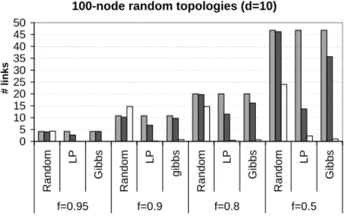
Figure 2 shows the simulation results for 100-node

100-node random topologies (d=10)

0 5 10 15 20 25 30 35 40 45 50 R a n d o m _LP G ib b s R a n d o m _LP g ib b s R a n d o m _LP G ib b s R a n d o m _LP G ib b s f=0.95 f=0.9 f=0.8 f=0.5 # li n k s

"# true lossy links" "# correctly identified lossy links" "# false positive"

Fig. 2. Varyingf: 100-node random topologies with maximum degree = 10.

topologies andd= 10, andfvarying from 0.5 to 0.95. We note that in general, random sampling has the best cover-age. In most cases, it is able to identify over 90-95% of the lossy links. However, the high coverage comes at the cost of a very high false positive rate — ranging from 50-140%. Such a high false positive rate may be manageable when there are few lossy links in the network (i.e., f is large) since we can afford to run more expensive tests (e.g., ac-tive probing) selecac-tively on the small number of lossy links inferred. However, the large false positive rate is unaccept-able when there are a large number of lossy links in the network. For instance, whenf = 0.5, random sampling correctly identifies 46 of the 47 lossy links. In addition, however, it generates 24 false positives, which makes the inference almost worthless since there are only about 100 links in all.

One reason why random sampling generates a large number of false positives is its susceptibility to statisti-cal fluctuations in the end-to-end loss rate experienced by clients (Section IV-B). For instance, instead of cor-rectly identifying a lossy link high up in the tree, random sampling may incorrectly identify a large number of links close to individual clients as lossy.

In contrast to random sampling, LP has relatively poor coverage (30-60%) but an excellent false positive rate (rarely over 5%). (In some cases, the false positive bar in Figure 2 is hard to see because the number of false pos-itives is close to or equal to zero.) As explained in Sec-tion IV-C, LP is less susceptible to statistical fluctuaSec-tions in the end-to-end loss rates since it allows some slack in the constraints. This cuts down the false positive rate. How-ever, the slack in the constraints and the fact that the objec-tive function assigns equal weights the link loss variables (Li) and the slack variables (Sj) causes a reduction in cov-erage. Basically, a true lossy link (especially one near the leaves) may not be inferred as such because the constraint

was slackened sufficiently to obviate the need to assign a high loss rate to the link. In Section V-C, we examine the impact of different weights in LP on the inference.

Finally, we observe that Gibbs sampling has a very good coverage (over 80%) and also an excellent false positive rate (well under 5%). We believe that the excellent per-formance of this technique arises, in part, because the Bayesian approach is based on observations of packet loss events and not the (noisy) computation of packet loss rates.

1000-node random topologies (d=10, f=0.95)

0 20 40 60 80 100 120 140 160 Random LP Gibbs # li n k s

"# true lossy links" "# correctly identified lossy links" "# false positive"

Fig. 3. 1000-node random topologies with maximumdegree= 10andf = 0.95.

1000-node random topologies (d=10, f=0.5)

0 100 200 300 400 500 600 Random LP Gibbs # li n k s

"# true lossy links" "# correctly identified lossy links" "# false positive"

Fig. 4. 1000-node random topologies with maximumdegree= 10andf = 0.5.

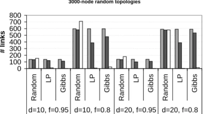
Figures 3 and 4 show the corresponding results for ex-periments on 1000-node topologies. Figure 5 shows the re-sults for 3000-node topologies. We observe that the trends remain qualitatively the same even for these larger topolo-gies. Gibbs sampling continues to have good coverage with less than 5% false positive.

Figure 6 shows the how accurate the inference based on Gibbs sampling is when the links inferred as lossy are rank ordered based on our “confidence” in the inference. We quantify the confidence as the fraction of Gibbs sam-ples that exceed the loss rate threshold set for lossy links. The 983 links in the topology are considered in order of decreasing confidence. We plot 3 curves: the true number

3000-node random topologies

0 100 200 300 400 500 600 700 800 R a n d o m _LP G ib b s R a n d o m _LP G ib b s R a n d o m _LP G ib b s R a n d o m _LP G ib b s d=10, f=0.95 d=10, f=0.8 d=20, f=0.95 d=20, f=0.8 # li n k s

# true lossy links # correctly identified lossy links # false positive

Fig. 5. 3000-node random topologies. Gibbs sampling for a 1000-node random topology (d = 10, f = 0.5) 0 100 200 300 400 500 600 0 200 400 600 800 1000 # li n k s

"# correctly identified lossy links" "# true lossy links" "# false positive"

Fig. 6. The performance of Gibbs sampling when the inferences are rank ordered based on a confidence estimate. (1000-node random topology, maximum degree = 10, andf =

0.5)

of lossy links in the set of links considered up to that point, the number of correct inferences, and the number of false positives. We note that the confidence rating assigned by Gibbs sampling works very well. There are zero false pos-itives for the top 33 rank ordered links. Moreover, each of the first 401 true lossy links in the rank ordered list is correctly identified as lossy (i.e., none of these true lossy links is “missed”). These results suggest that the confi-dence estimate for Gibbs sampling can be used to rank the order of the inferred lossy links so that the top few infer-ences are (almost) perfectly accurate. This is likely to be useful in a practical setting where we may want to identify at least a small number of lossy links with certainty so that corrective action can be taken.

B. Alternative Loss Model

So far, we have considered LM1 loss model with the

Bernoulli loss process. In this section, we evaluate the ef-fectiveness of inference using alternatives for both (i.e., the LM2 loss model and the Gilbert loss process) in various combinations.

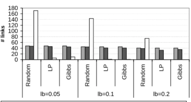
LM₂ Bernoulli loss model: Figure 7 shows the results

for 1000-node random topologies withd = 10and f =

rate threshold, lb, used to decide whether a link is lossy. We observe that the coverage is well over 80% for all the algorithms. As the loss threshold is increased, the false positive rate decreases while the coverage remains high. This suggests that the inference can be more accurate if we are only interested in highly lossy links.

1000-node random topologies with LM2 Bernoulli link loss model

0 20 40 60 80 100 120 140 160 180 R a n d o m _LP G ib b s R a n d o m _LP G ib b s R a n d o m _LP G ib b s lb=0.05 lb=0.1 lb=0.2 # li n k s

True lossy links # correctly identified lossy links # false positive Fig. 7. ALM2 Bernoulli loss model for 1000-node random

topologies with maximumdegree = 10andf = 0.95. We vary the loss thresholdlb, and only the links with loss rate higher thanlbare considered lossy.

LM1andLM2Gilbert loss models: Figure 8 and

Fig-ure 9 show the performance of inference for LM1 and

LM2 Gilbert loss models. The relative performance of

different inference schemes remains the same. The Gibbs sampling continues to be the best performer: it has around 90% coverage with the lowest false positive among all the schemes.

1000-node random topologies with LM1 Gilbert loss model

0 20 40 60 80 100 120 140 160 180 Random LP Gibbs # li n k s

# true lossy links # correctly identified lossy links # false positive Fig. 8. A LM1 Gilbert loss model for 1000-node random

topologies with maximumdegree= 10andf = 0.95.

C. Different Weights in LP

The linear optimization algorithm aims to minimize wP_iLi+

P

j|Sj|, where the weight,w, reflects the rel-ative importance between finding a parsimonious solution versus satisfying the end-to-end loss constraints. So far in our experiments, we usew= 1. In this section, we varyw and examine its effect on the performance of the inference.

1000-node random topologies with LM2 Gilbert loss model

0 10 20 30 40 50 60 70 80 90 100 R a n d o m _LP G ib b s R a n d o m _LP G ib b s R a n d o m _LP G ib b s lb=0.05 lb=0.1 lb=0.2 # li n k s

# true lossy links # correctly identified lossy links # false positive Fig. 9. A LM2 Gilbert loss model for 1000-node random

topologies with maximumdegree = 10andf = 0.95. We vary the loss thresholdlb, and only the links with loss rate higher thanlbare considered lossy.

Figure 10 and Figure 11 show the LP performance for 1000-node random topologies under GilbertLM1 and LM2 loss models, respectively. As we can see, the lower

thew, the better coverage the inference achieves, but at the cost of higher false positive rates. This is because when we decrease the weight, we emphasize more on satisfying the constraints than finding a parsimonious solution; as a result, we are more likely to attribute loss to several non-shared links than a single non-shared link in order to satisfy the constraints more closely. Moreover it is interesting that the performance of LP is less sensitive to the weights in theLM2loss model than in theLM1loss model.

1000-node random topologies with LM1 Gilbert loss model

0 10 20 30 40 50 60 70 80 LP(0.5) LP(1) LP(2) # li n k s

# true lossy links # correctly identified lossy links # false positive Fig. 10. Effects of different weights in LP: ALM1 Gilbert

loss model for 1000-node random topologies with maxi-mumdegree= 10andf = 0.95.

D. Real Topology

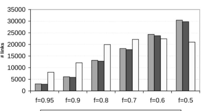
We also evaluate the effectiveness of inference using a real topology (constructed from traceroute data) spanning 123,166 clients. We assign a loss rate to each link based on theLM1Bernoulli loss model with different settings of f. Figure 12 shows the performance of random sampling. As with the random topologies, random sampling has very

1000-node random topologies with LM2 Gilbert loss model

0 10 20 30 40 50 60 L P (0 .2 5 ) L P (0 .5 ) L P (0 .7 5 ) L P (1 ) L P (2 ) L P (0 .2 5 ) L P (0 .5 ) L P (0 .7 5 ) L P (1 ) L P (2 ) L P (0 .2 5 ) L P (0 .5 ) L P (0 .7 5 ) L P (1 ) L P (2 ) lb=0.05 lb=0.1 lb=0.2

# true lossy links # correctly identified lossy links # false positive

Fig. 11. Effects of different weights in LP: ALM2 Gilbert

loss model for 1000-node random topologies with maxi-mumdegree= 10andf = 0.95. We vary the loss thresh-oldlb, and only the links with loss rate higher thanlbare considered lossy.

good coverage but a significant false positive rate. Real topology (random sampling)

0 5000 10000 15000 20000 25000 30000 35000 f=0.95 f=0.9 f=0.8 f=0.7 f=0.6 f=0.5 # li n k s

"# true lossy links" "# correctly identified lossy links" "# false positive"

Fig. 12. Real topology from the Dec 2000 traceroute. We were unable to evaluate the performance of LP and Gibbs sampling over the real topology because of compu-tational complexity.

VI. INTERNETRESULTS

In this section, we evaluate the passive tomography techniques using the Internet traffic traces from mi-crosoft.com. Validating our inferences is challenging since we only have end-to-end performance information and do not know the true link loss rates. The validation approach we use is to (i) check consistency in the inferences made by the three techniques, (ii) look at the characteristics of in-ferred lossy links, and (iii) examine whether clients down-stream of an inferred lossy link do in fact experience high loss rates.

The evaluation we present here is based on a tcpdump trace we gathered on 20 Dec 2000. This trace was 2.12 hours long and contained 100 million packets to or from 134,475 clinets. To compute loss rate, we only consider clients that receive at least a threshold number of packets,

t, which is set to 500 or 1000 packets in our evaluation. A. Consistency across different schemes

First, we examine the consistency in the lossy links identified by the three tomography techniques. Figure 13 shows the amount of overlap when we consider the topN lossy links found by different schemes. Gibbs sampling and random sampling yield very similar inferences, with an overlap that is consistently above 95% whenN is var-ied from 1 to 100.5The overlap between LP and the other techniques is also significant — over 60%.

0 10 20 30 40 50 60 70 80 90 100 0 20 40 60 80 100 120 N O v e rl a p in th e to p N id e n ti fi e d lo s s y li n k s

Random vs. Gibbs sampling LP vs. Gibbs sampling Random vs. LP All

N

Fig. 13. Overlap in the top N lossy links identified by different schemes.

B. Characteristics of Inferred Lossy Links

In this section, we examine the characteristics of the in-ferred lossy links. We are interested in knowing the loca-tion of the inferred lossy links in the Internet topology. As shown in Figure 14, more than 95% of lossy links detected through random sampling and Gibbs sampling terminate at leaves (i.e., clients). In other words, these are non-shared links that include the physical last-hop link to clients. (Re-call from Section IV-A that the tomography techniques operate on virtual links, which may span multiple physi-cal links.) Even though the linear optimization technique is biased toward ascribing lossiness to shared links, more than 75% of the inferred lossy links are non-shared links terminating at clients. These findings are consistent with the common belief that the last mile to clients is often the bottleneck in Internet paths [6]. Since many losses happen at non-shared links, it is not surprising that there is only a limited degree of spatial locality in end-to-end loss rate, as reported in Section III

We also examine how many of the links inferred to be lossy cross AS boundaries since such crossings (such as

5

This overlap is higher than we had expected, since random sampling has a relatively high false positive rate in our simulations. As we de-scribe in Section VI-B, most lossy links terminate at leaves and most internal links are not lossy. So clients whose last hop links are not lossy experience little or no loss. This places tighter constraints on the space of feasible solutions, which makes random sampling more accurate.

Number of leaves among the top 100 identified lossy links

0 10 20 30 40 50 60 70 80 90 100 Random LP Gibbs # li n k s te rm in a te a t le a v e s t=1000 t=500

Fig. 14. Number of lossy links that terminate at leaf nodes.

peering points) are thought to be points of congestion. We find that among all the virtual links in our topology (each of which may include multiple physical links), around 45% cross AS boundaries, and 45% have roundtrip delay (i.e., the delay between the two ends of the virtual link as determined from the traceroute data) over 100 ms. When we consider only the inferred lossy virtual links, the per-centage of links that cross AS boundaries or have long de-lay is considerably higher. For example, if we only con-sider those links with an inferred loss rate above 10%, 70% cross AS boundaries, and 80% have one-way delay over 100 ms. Some examples of such links we found include the connection from AT&T in San Francisco to IndoInt-ernet in Indonesia (inter-ISP and transcontinental), from Sprint to Trivalent (inter-ISP), and an international link in ChinaNet from U.S. to China.

C. Trace-driven Validation

We now consider the problem of validating our infer-ences more directly than the intuitive arguments made in Section VI-B. This is a challenging problem since we do not know the true loss rates of Internet links. (All the in-ferences were made offline. So we could not validate the results using active probing.)

We have developed the following approach for valida-tion. We partition the clients in the trace into two groups: tomography set and validation set. The partitioning is done by clustering all clients according to BGP address prefixes and dividing each cluster into two sets. One set is included in the tomography set and the other in the validation set. This partitioning scheme ensures that there is a significant overlap in the end-to-end path to clients in the two sets.

We apply the inference techniques to the tomography set to identify lossy links. For each lossy link that is iden-tified, we examine whether clients in the validation set that are downstream of that link experience a high loss rate on average. If they do, we deem our inference to be correct. Otherwise, we count it as a false positive. Clearly, this val-idation method can only be applied to shared lossy links.

Ll Method t Ni Nc 4% Rand 1000 5 5 Rand 500 5 4 LP 1000 8 5 LP 500 11 6 2% Rand 1000 11 10 Rand 500 14 13 LP 1000 22 14 LP 500 24 20 1% Rand 1000 24 17 Rand 500 23 19 LP 1000 46 28 LP 500 106 77 TABLE I

TRACE-DRIVEN VALIDATION FOR RANDOM SAMPLING AND LINEAR OPTIMIZATION.

We cannot use this method to validate the many “last-hop” lossy links reported in Section VI-B.

Table I shows our validation results for random sam-pling and linear optimization, where Ll is the loss rate threshold we used to deem a link to be lossy,tis the mini-mum number of packets a client should have received to be considered in the tomography computation,Niis the num-ber of inferred (shared) lossy links, andNcis the number of correct inferences according our validation method. In most cases random sampling and linear optimization have a false positive rate under 30%. Gibbs sampling identi-fied only 2 shared lossy links, both of which are deemed correct according to our validation method.

VII. CONCLUSIONS

In this paper, we present a study of wide-area Inter-net performance as observed from the busy microsoft.com Web site. We characterize the end-to-end loss rate expe-rienced by clients and present techniques to identify lossy links within the network based on passive monitoring of existing client-server traffic.

We find that the end-to-end packet loss rate correlates poorly with topological distance (i.e., hop count), remains stable for several minutes, and exhibits a limited degree of spatial locality.

These findings suggest that passive network tomogra-phy would be both useful and feasible. We develop and evaluate three different techniques for passive network tomography: random sampling, linear optimization, and Bayesian inference using Gibbs sampling. In general, we find that random sampling has the best coverage but also

a high false positive rate, which can be problematic when the number of lossy links is large. Linear optimization has a very low false positive rate but only a modest coverage. Gibbs sampling offers the best of both worlds: a high cov-erage (over 80%) and a low false positive rate (below 5%). On the flip side, however, Gibbs sampling is computa-tionally the most expensive of our techniques. On the other hand, random sampling is the quickest one. Therefore, we believe that random sampling may still be useful in prac-tice despite its high false positive rate. For instance, when the number of lossy links in (the portion of) the network of interest is small, it may be fine to apply random sampling since the number of false positives (in absolute terms) is likely to be small. Furthermore, if the number of lossy links is large (for instance, thef = 0.5configurations in Section V), it is a moot question as to whether network tomography will be very useful.

In addition to simulation, we have applied some of our tomography techniques to Internet packet traces. The main challenge is in validating our inferences. We validate the inference by first checking consistency across the results from different schemes. We find over 95% overlap be-tween the top 100 lossy links identified by random sam-pling and Gibbs samsam-pling, and over 60% overlap between LP and the other two techniques. We also find that most of the links identified as lossy are non-shared links terminat-ing at clients, which is consistent with common belief. Fi-nally we develop an indirect validation scheme, and show the false positive rate is manageable (below 30% in most cases and often much lower).

We are presently investigating an approach based on se-lective active probing to validate the findings of our pas-sive tomography techniques. To this end, we are working on making inferences in real time.

REFERENCES

[1] M. Allman. A web server’s view of the transport layer. ACM Computer Communication Review, October 2000.

[2] H. Balakrishnan, S. Seshan, M. Stemm, and R. H. Katz. Analyz-ing stability in wide-area network performance. In ProceedAnalyz-ings of ACM SIGMETRICS’98, June 1997.

[3] R. Caceres, N. G. Duffield, J. Horowitz, D. Towsley, and T. Bu. Multicast-based inference of network internal characteristics: Ac-curacy of packet loss estimation. In Proceedings of IEEE INFO-COM’99, March 1999.

[4] A. Downey. Using pathchar to estimate internet link characteris-tics. In ACM SIGCOMM, 1999.

[5] N. G. Duffield, F. Lo Presti, V. Paxson, and D. Towsley. Inferring link loss using striped unicast probes. In Proceedings of IEEE INFOCOM’2001, April 2001.

[6] C. Fraleigh, S. Moon, C. Diot, B. Lyles, and F. Tobagi. Packet-level traffic measurements from a tier-1 ip backbone. In Under submission, November 2001.

[7] S. Geman and D. Geman. Stochastic relaxation, gibbs

distribu-tions and the bayesian restoration of images. In IEEE Trans. Pattn. Anal. Mach. Intel., 1984.

[8] W. R. Gilks, S. Richardson, and D. J. Spiegelhalter. Markov Chain Monte Carlo in Practice. 1996.

[9] V. Jacobson. Traceroute software. 1989.

[10] D. Katabi, I. Bazzi, and X. Yang. A passive approach for detecting shared bottlenecks, October 2001.

[11] J.C. Mogul, F. Douglis, A. Feldman, and B. Krishnamurthy. Po-tential benefits of delta-encoding and data compression for http. In Proceedings of ACM SIGCOMM ’97, Sept. 1997.

[12] E. M. Nahum, C.-C. Rosu, S. Seshan, and J. Almeida. The effects of wide-area conditions on www server performance. In Proceed-ings of ACM SIGMETRICS, June 2001.

[13] J. Padhye, V. Firoiu, D. Towsley, and J. Kurose. Modeling tcp throughput: A simple model and its empirical validation. In Pro-ceedings of ACM SIGCOMM’98, August 1998.

[14] V. N. Padmanabhan, L. Qiu, and H. J. Wang. Server-based in-ference of internet performance. In Microsoft Research Technical Report MSR-TR-2002-39, May 2002.

[15] V. Paxson. Measurements and analysis of end-to-end internet dy-namics. In Proceedings of ACM SIGCOMM ’97, Sept. 1997. [16] S. Ratnasamy and S. McCanne. Inference of multicast routing

trees and bottleneck bandwidths using end-to-end measurements. In Proceedings of IEEE INFOCOM 1999, 1999.

[17] D. Rubenstein, J. Kurose, and D. Towsley. Detecting shared con-gestion of flows via end-to-end measurement. In Proceedings of ACM SIGMETRICS, 2000.

[18] S. Seshan, M. Stemm, and R. H. Katz. SPAND: Shared passive network performance discovery. In Proceedings of 1st Usenix Symposium on Internet Technologies and Systems (USITS ’97), December 1997.

[19] Y. Tsang, M. J. Coates, and R. Nowak. Passive network tomog-raphy using em algorithms. In Proceedings of the IEEE Interna-tional Conferenceon Acoustics, Speech, and Signal Processing, May 2001.

[20] Y. Zhang, N. Duffield, V. Paxson, and S. Shenker. On the con-stancy of internet path properties. In Proceedings of ACM SIG-COMM Internet Measurement Workshop, November 2001. [21] Y. Zhang, V. Paxson, and S. Shenker. The stationarity of internet

path properties: Routing, loss, and throughput. In ACIRI Techni-cal Report, May 2000.