COMPUTATION OF UNSTEADY MHD MIXED CONVECTIVE HEAT AND MASS TRANSFER IN DISSIPATIVE REACTIVE MICROPOLAR FLOW CONSIDERING SORTE AND DUFOUR EFFECTS

COMPUTATION OF UNSTEADY MHD MIXED CONVECTIVE HEAT AND

MASS TRANSFER IN DISSIPATIVE REACTIVE MICROPOLAR FLOW

CONSIDERING SORET AND DUFOUR EFFECTS

M.D. Shamshuddin

a*

_{, A.J. Chamkha}

b,c

_{, Thirupathi Thumma}

d

_{, M.C. Raju}

e

a _{Department of Mathematics, Vaagdevi College of Engineering (Autonomous) Warangal, Telangana-506005, India.}

b_{Mechanical Engineering Department, Prince Mohammad Bin Fahd University, Al-Khobar 3192, Saudi Arabia}

c_{Prince Sultan Endowment for Energy and Environment, Prince Mohammad Bin Fahd University, Al-Khobar 31952, Saudi Arabia} d _{Department of Mathematics, B V Raju Institute of Technology, Medak, Telangana-502313, India}

.

e_{Department of Mathematics, Annmacharya Institute of Technology and Sciences (Autonomous) Rajampet, Andhra Pradesh-516126, India}

A

BSTRACT

In the current paper, a finite element computational solution is conducted for MHD double diffusive flow characterizing dissipative micropolar mixed convective heat and mass transfer adjacent to a vertical porous plate embedded in a saturated porous medium. The micropolar fluid is also chemically reacting, both Soret and Dufour effects and also heat absorption included. The governing partial differential equations for momentum, heat, angular momentum and species conservation are transformed into dimensionless form under the assumption of low Reynolds number with appropriate dimensionless quantities. The emerging boundary value problem is then solved numerically with an efficient computational finite element method employing the weighted residual approach. The influence of various emerging physical parameters like thermal Grashof number, solutal Grashof number, Magnetic body force parameter, permeability parameter, radiation parameter, heat absorption parameter, Eckert number, Schmidt number, Soret and Dufour effects and first order chemical reaction parameter are examined, we observed that the microrotation velocity profiles do not show uniform variations with Eringen vortex viscosity parameter and graphical results visualize the velocity of a Newtonian fluid is lower as compared with a micropolar fluid one. Furthermore, finite element code is benchmarked with the results reported in the literature to check the validity and accuracy under some limiting cases and excellent agreement is seen with published solutions. Finally, results of skin friction coefficient, couple stress coefficient, Nusselt number and Sherwood number for invoked parameter are tabulated which shows that Sherwood number is enhances with increasing Soret number and homogeneous chemical reaction. Nusselt number is increasedwith an increase of Eckert number and Dufour number.

Keywords: Soret- Dufour effects, chemical reaction, micropolar fluid, mixed convection, finite element method.

1. INTRODUCTION

Modern fluid dynamics is an area of research provides a multi-disciplinary plat form for theoretical computational based investigations. Different materials exist which exhibit a considerable range of shear-stress strain relational ship which does not obey classical Newtonian fluids i.e. Navier-Stokes equation, which are called as polar fluids. Development in this area was pioneered by Eringen (1996), also Eringen (1972) provided summary of thermodynamics and hydro-dynamics of micropolar fluid Eringen (2001). Interesting aspects of theory and applications of micropolar fluids can be found in book by Lukaswiascz (1999), review articles by Ariman et al. (1973, 1974). These investigations have addressed numerous multi-physical phenomena including thermal dispersion, thermal radiation, electrophoresis, wavy surfaces, body rotations, oscillatory flow, squeezing hydrodynamics, fluid dynamic stability and magnetohydrodynamics. Micro-inertia itself is not important, some properties of microstructure do play vital role in determining the structure of boundary layer Peddieson (1968), Na and Pop (1997). Gupta et al. (2014) presented finite element analysis for microstructural boundary layer flow over stretching sheet. Recently, Bilal et al. (2017) demonstrated the boundary layer flow of magneto-micropolar nanofluid.

* _{Corresponding author. Email : [email protected] (or) [email protected]}

A Wide range of research has been implemented to study magnetohydrodynamics (MHD) effects in different fluids at different situations, which deals the interaction of conducting fluids with electromagnetic phenomena. Heat transfer flow of an electrically conducting micropolar fluid under influence of magnetic field on boundary layer in porous and non-porous media is exploited in numerous modern industrial processes including energy generators, ionized propulsion system, vortex control Chen et al. (2012) etc. Magento-micropolar flow are therefore greatly relevant to such systems. Pal and Talukdar (2012) used a perturbation technique to investigate unsteady MHD mixed convection periodic flow, heat and mass transfer in micropolar fluid with chemical reaction in the presence of thermal radiation. Reddy (2012) investigated magnetohydrodynamic and unsteady convection flow of micropolar fluid past a vertical porous plate with variable wall heat flux and also studied an unsteady magnetohydrodynamic radiative-convective flow of a micropolar fluid past a vertical porous plate with variable heat and mass fluxes Reddy (2013). Gupta et al. (2014) who used a variational finite element method to investigate strong radiative flux in both free and forced convection of micropolar liquids. However, it is worthwhile to mention the contribution made by several authors in this regard with numerical or analytical approach are Hayat and Qasim (2014) used Homotopy analysis to study thermal radiation effects on magnetohydrodynamic flow of micropolar fluid. Gupta et al. (2014) used variational finite element method to study

Frontiers in Heat and Mass Transfer

mixed convection flow of micropolar fluid over stretching sheet. Hayat et al. (2016) investigated magnetohydrodynamic peristaltic flow of micropolar fluid in curved channel, further Hayat et al. (2017) analyzed the magnetohydrodynamic flow of micropolar fluid over curved stretching surface. Recently, Bakr and Chamkha, (2016) employed small perturbation technique to investigate effects of variable heat flux and thermal radiation in rotating micropolar fluid. Ahmad et al. (2017) used Laplace transform technique to examine magnetohydrodynamic flow of micropolar fluid over oscillating vertical plate. Srinivasa Raju et al. (2016) studied both numerical and analytical solutions for exponentially moving vertical plate. Srinivasa Raju et al. (2017), Srinivasa Raju et al. (2017) used finite element method to examine Casson fluid flow over an inclined plate. Viscous dissipation term is conventionally neglected in most of investigations because of Eckert number is small based on an order of magnitude analysis, hence study of viscous dissipation is important in various physical aspects who consider are Han and Lee (2007) examined viscous dissipation effects in micro-channel theoretically in a fully developed laminar flow region. Das (2014) conducted a numerical investigation in magnetohydrodynamic mixed convection flow under chemical reaction and viscous dissipation effects. Siva reddy and Shamshuddin (2015) presented viscous dissipation effects in rotating micropolar fluid. Singh and Kumar (2016) numerically investigated the thermal radiation, viscous dissipation and heat generation or absorption effects over stretching surface of a micropolar fluid.

In the above investigations, the effect of Soret and Dufour in hydromagnetics has been excluded. However, in many physico-chemical heat and mass transfer studies, related to both Newtonian and non-Newtonian fluids, thermo-diffusion (Soret) and diffuso-thermo (Dufour) effects play a prominent role. These effects are often of smaller order of magnitude in comparison with the diffusive effects associated with thermal conduction (Fourier’s law) and mass diffusion (Fick’s laws) and are frequently neglected. However, these so-called cross diffusion effects become important if not dominant, in materials processing operations e.g. dendritic growth (Tsai and Huang, 2009), MHD power generators, magnetic separation of colloids, and aerospace combustion and flame dynamics where they arise in binary gas and supercritical fuel injection systems. Generally, when heat and mass transfer effects occur simultaneously in a moving fluid, the relationship between the fluxes and the driven potentials become significant. An energy flux can be generated not only by temperature gradient but also by composition gradient as well. The energy caused by a composition gradient is called the Dufour effect or diffusion- thermo effect. The energy caused by a temperature gradient is called the Soret effect or thermo-diffusion effect. The thermal Soret effect can for example also generate a very strong coupling force between the species (solute) and heat transport. Due to the significance importance of Soret and Dufour diffusion phenomena for fluids with medium molecular weight as well as very light molecular weights, in recent years’ substantial interest has emerged in simulation of these effects in many multi-physical transport problems. Postelnicu (2004) considered magnetic free convection in porous media with Soret and Dufour effects. Alam and Rahman (2005) investigated combined Dufour and Soret effects on hydromagnetic natural convection flow in a porous medium. Further studies of Newtonian flows with Soret/Dufour effects include Partha et al. (2006) for non-Darcian thermal convection, Alam and Ahammed (2011) for variable heat and mass flux effects, and (Aurangzaib et al. 2013) for mixed convection stagnation point flow, Srinivas Raju et al. (2016), Jithender Reddy et al. (2017) for vertical and inclined plates. Non-Newtonian heat and mass transfer with Soret and/or Dufour effects has also attracted some attention. Odelu and Naresh kumar (2016) used a quasi-linearization technique for mixed convection flow of micropolar fluid between porous parallel plates with soret and dufour effects. Other representative studies include Kundu et al. (2015) Shamshuddin (2016), Shamshuddin and Thirupathi (2017) for micropolar fluids.

In the present investigation, we generalize and extend existing studies Reddy (2012, 2013) to consider the combined effects of Soret and Dufour cross diffusion, heat absorption, first order chemical reaction and viscous dissipation on radiative magnetohydrodynamic micropolar flow, heat and mass transfer from a vertical plate adjacent to a porous medium with variable heat and mass fluxes. The non-dimensional conservation equations are solved with a finite element method. The effect of various physical parameters on the velocity, micro-rotation velocity, temperature and concentration profiles as well as on local skin friction coefficient, wall couple stress, Sherwood number and Nusselt number are tabulated. Validation of the analysis has been performed by comparing the present results with those of Reddy (2013). The current study is relevant to high temperature electromagnetic rheological flows in energy generators and magneto-rheological materials fabrication systems (where thermal radiation heat transfer is also significant) and has not appeared in technical literature thus far.

2. MATHEMATICAL MODELLING

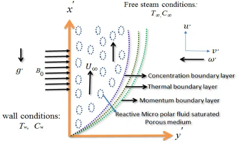
Consider the two-dimensional, unsteady free convection flow of an incompressible and electrically-conducting micropolar fluid, heat and mass transfer from an infinite vertical moving porous plate suspended in a homogenous, isotropic, porous medium. The physical configuration is illustrated in Fig. 1. The vertical plate is assumed to be subjected to a constant heat flux, q_w and a constant concentration gradient,

m

_w

. A

magnetic field of uniform strength B0is applied in a direction parallel

to the y′_{axis which is perpendicular to the flow direction. It is assumed}

that the induced magnetic field is negligible in comparison to the applied magnetic field, Cowling (1957). Magnetic Reynolds number is very small. The MHD term is derived from an order of magnitude analysis of the full Navier-Stokes equation.

Before we derive the governing equations, the following assumptions are made, incompressible flow, time dependent flow, mixed convection flow, unidirectional flow, non-Newtonian flow, Darcy’s law is assumed and low Reynolds number flow, applied or polarized voltage is neglected so that no energy is added or extracted from the fluid by electrical means, fluid is gray-absorbing-emitting but non-scattering medium, Rosseland approximation is used to describe radiative heat flux

in x′direction is considered negligible in comparison with that of y′

direction, heat generation and viscous dissipation is present as are Soret and Dufour effects, Ohmic dissipation is ignored, magnetic micropolar fluid contains a species which is reactive and obeys first order chemical. To simplify the formulation of the boundary conditions, we assumed the size of holes in the porous plate is significantly larger than the characteristic microscopic length scale of the micropolar fluid. It is assumed that the plate is infinite in extent and hence all physical quantities depend only ony′and

t

′

.

The governing equations by usingBoussinesq approximation for this investigation are based on the balances of mass, linear momentum, energy, and concentration species. Taking into consideration the assumptions made above, these equations can be written in Cartesian frame of reference, as follows:

0 = ′ ∂ ′ ∂ y v

(1)

(

)

(

)

(

)

( )

y r u B K u C w C c g T w T f g y u r x p z u v t u ′ ∂ ′ ∂ + ′ − ′ ′ − ∞′ − ′ + ∞′ − ′ + ′ ∂ ′ ∂ + + ′ ∂ ′ ∂ − = ′ ∂ ′ ∂ ′ + ′ ∂ ′ ∂ ω ν ρ σ ν β β ν ν ρ 2 2 0 2 2 1

(2)

2 2 y o y v t j ′ ∂ ′ ∂ =           ′ ∂ ′ ∂ ′ + ′ ∂ ′ ∂ ′ ω ω γ ω

ρ

(3)

(

)

2 2 2 1 2 2 y C cp cs T K m D y u p C T w T p C Q y r q p C y T p C y T v t T ′ ∂ ∂ +       ′ ∂ ′ ∂ + ∞′ − ′ ′ −           ′ ∂ ∂ −           ′ ∂ ∂ = ′ ∂ ∂ ′ + ′ ∂ ∂ ρ µ ρ ρ ρ κ

(4)

(

′ − _∞′

)

′ −           ′ ∂ ∂ +           ′ ∂ ∂ = ′ ∂ ∂ ′ + ′ ∂ ∂ C w C r K y T m T t K m D y C m D y C v t C 2 2 2 2

(5)

It is assumed that the porous plate moves with a constant velocity in the longitudinal direction, the free stream velocity follows an exponentially increasing (or) decreasing deviate slightly and the plate temperature and suction velocity differ exponentially with time, under these assumptions following spatial and temporal boundary conditions are: ∞ → ′     ∞ ′ → ′ ∞′ → ′ → ′       ₊ ′′ = ∞′ → ′ > ′ = ′               ₊ ′′ − = = ′       ′ ∂ ∂       ₊ ′′ − = = ′       ′ ∂ ∂ ′ ∂ ′ ∂ − = ′ = ′ ≤ ′ y for C w C , T w T , , t n e o U U u : t and y for t n Ee m D w m y y C , t n Be w q y y T , y u , u : t 0 1 0 0 1 0 1 0 2 1 0 0 ω ε ε ε κ ω

(6)

where Band E are real positive constants.

ε

is a small quantity,

such that

ε

B

<<

1

,

ε

E

<<

1

and

n

′

is constant. Integrating the mass conservation (continuity) equation (1) for variable suction velocity normal to the plate we consider a convenient solution to be:

      ′′ + − =

′ V Aent

v ₀1 ε

(7)

where A is real constant such that

ε

A

<<

1

and V0 is the normal velocity at the plate, negative sign indicates the suction velocity is directed towards the plate. Following Rosseland’s approximation (Brewster, 1992), the radiative heat flux term is given by

        ′ ∂ ∂ − = y T k r q 4 3 4σ

(8)

The assumed Rosseland model is quite accurate for optically-thick media for the present analysis where thermal radiation propagates a limited distance prior to encountering scattering or absorption. The refractive index of the fluid-particle suspension is assumed to be constant, intensity within the fluid is nearly isotropic and uniform and wavelength regions exist where the optical thickness is usually in excess

of five also eqn. (8) results in a highly nonlinear energy equation inTand it is difficult to obtain a solution. However, researchers have resolved this problem by assuming small temperature differences with in the fluid flow Adunson and Gebhert (1972), Raptis and Perdikis (1998). In this situation, Rosseland’s model can be linearized about ambient temperature T∞′ assuming that the difference in the temperature with in the flow such that T′4can be expressed as linear combination of the temperature. Using Taylor’s series expansion about T′ the expansion of

4

T′ can be written as follows, neglecting higher order terms:

(

T T

)

T

(

T T

)

...

T T

T′4= _∞′4+4 _∞′3 ′− _∞′ +6 _∞′2 ′− _∞′ 2+

(9) Neglecting higher order terms beyond the first degree in

(

T′−T_∞′

)

, we have 4 3 3 4 4 ∞′ − ∞′ ≅

′ T T T

T

(10)

Differentiating equation (8) w.r.t y′and using (10), we obtain:

2 2 3 3 16 y T k T y r q ′ ∂ ∂ ∞ − − = ′ ∂ ∂ σ

(11)

Now simply replacing T3in Eq. (8) withT∞3, Eq. (4) can be expressed

as follows:

(

)

2 2 2 2 2 3 3 16 1 y C cp cs T K m D y u p C T w T p C Q y T T k p C t T ′ ∂ ∂ +       ′ ∂ ′ ∂ + ∞′ − ′ ′ − ′ ∂ ∂         ∞ + =         ′ ∂ ∂ ρ µ ρ κ σ ρ κ (12)

Outside the boundary layer Eq. (2) gives

∞ ′ + ∞′ ′ + ′ ∞ ′ = ′ ′

− U BoU

K t d U d x d p d ρ σ ν ρ 2 1 (13)

Introducing the following non-dimensional variables:

(

)

(

)

(

(

)

)

(

)

(

)

(

)

                                     ′ = = = ∞′ − ′ = ′ = ∞ = = ∞ ′ − ′ = ∞′ − ′ = = = ′ = = Λ = + ′ = ′ Λ + = ′ = ∞ ′ − ′ ∞ ′ − ′ = ∞′ − ′ ∞′ − ′ = ′ = ′ = ∞ ′ = ∞ ′ = ′ = ′ = ′ = , o V v r K , w m m T w q T K m D Sr , cp cs w q w m T K m D u D , T w T p C o U Ec , o V Cp v Q H , k k T F , m D Sc , o V o U C w C c g Gm , o V o U T w T f g Gr , Cp Cp Pr , K o V K , V o B M , , j j , j V j , w m C w C m D V C C , w q T w T V k T T , V n n , V o U , U U U , V t t , y V y , V v v , V u u 2 2 2 3 3 16 2 2 2 2 2 0 2 2 1 2 0 2 2 0 0 0 2 0 0 0 2 0 0 0 0 γ κ ν ν ρ σ ν ν β ν β κ µ κ ρ ν ν ρ σ µ β β µ µ γ ν φ θ ν ω ν ω ν ν (14)

In view of Eqs (6) - (14) the governing equations (2) - (5) and dropping primes yields the following dimensionless equations:

2 2 1 1 y y nt Ae t _∂ ∂ = ∂ ∂       + − ∂ ∂ ω η ω ε ω (16)

(

)

          ∂ ∂ +       ∂ ∂ + + − ∂ ∂ + = ∂ ∂       + − ∂ ∂ 2 2 2 2 2 1 1 1 y Du y u Ec H y F Pr y nt Ae t φ θ θ θ ε θ (17) φ γ θ φ φ ε φ −           ∂ ∂ +           ∂ ∂ = ∂ ∂       + − ∂ ∂ 2 2 2 2 1 1 y Sr y Sc y nt Ae

t (18)

where j ,

β γ µ η + = ′ = 2 2 0

is the dimensionless gyro-viscosity

micropolar material parameter N=

(

M+

(

1/K

)

)

.The boundary conditions can be written in non-dimensional form as follows:

{

→ _∞ → → → →∞ >        =       + − =       ∂ ∂       + − =       ∂ ∂ ∂ ∂ − = = ≤ y for , , , U u : t and y for nt e E y , nt e E y , y u , u : t 0 0 0 0 0 1 1 2 1 0 0 φ θ ω ε φ ε θ ω

(19)

The mathematical statement of the problem is now complete and embodies the solution of Eqs. (15) -(18) focus to boundary conditions (19). Once the key variables are computed, a number of wall gradient functions may be automatically evaluated. For materials processing operations the physical quantities of principal interest are the wall skin-friction components (plate shear stress), wall couple stress components (micro-rotation gradient), Nusselt number (wall heat transfer rate) and Sherwood number (wall mass transfer rate):

, o V o U w f C ρ τ∗

= where

0 0

0  =

       ∂ ∂ = =         ∂ ∂ = ∗ y y u o V U y y u

w µ ρ

τ o U j w M m C µ

= where

0 = ∗         ∗ ∂ ∂ = y y w

M γ ω

In addition to that rate of heat transfer and rate of mass transfer at the

surface of wall are

0 = ∗         − ∞ ∂ ∂ = y w T T y / T x Nu _and 0 = ∗         − ∞ ∂ ∂ = y w C C y / C x Sh

The following skin friction, wall couple stress, Sherwood number and Nusselt number in non-dimensional for are

Skin-friction components are obtained as

0 =       ∂ ∂ = y y u f

C ₍₂₀₎

The couple stress coefficient at the plate, which in the non-dimensional form is given by

0 =       ∂ ∂ = y y m

C ω (21)

Nusselt number is computed as, which in the non-dimensional form is given by 0 =       ∂ ∂ − = y y x Re /

Nu θ (22)

Sherwood number is evaluated as, which in the non-dimensional form is given by

0 =       ∂ ∂ − = y y x Re /

Sh

φ

₍₂₃₎

whereRe_x=V_ox/ν is the Reynolds number.

3. GALERKIN FINITE ELEMENT NUMERICAL

SOLUTION

The finite element method (FEM) is employed to solve the transformed, coupled boundary value problem defined by eqns. (15)- (18) under (19). FEM is the most versatile technique available for engineering analysis and equally adept at handling ordinary or partial differential equations as well as integral equations. The general details of the variationalfinite element method are documented succinctly in (Reddy, 1985; Bathe, 1996). FEM has been applied to study many complex boundary value problems in micropolar fluid mechanics Norrie and De Vries (1978). Micropolar heat and mass transfer applications also include Beg et al. (2008), Bhargava et al. (2016). The fundamental steps involved in the finite-element analysis of a problem are as follows:

• Discretization of the infinite fluid domain into finite elements

• Derivation of element equations

• Assembly of Element Equations

• Imposition of boundary conditions

• Solution of assembled equations

The final matrix equation obtained can be solved by any efficient iterative scheme.

3.1 Variational Formulation

The variational formulation associated with Eqns. (15) - (18) over a typical two-node linear element

(

y_e,y_e+1

)

is given by:

(

)

0 1 4 2 2 3 2 1 1 = +                       ∂ ∂ − − ∞ − + −         ∂ ∂ − −       ∂ ∂ − ∂ ∂ dy e y e y y A u U N ) Gm Gr ( y u A A y u A t u w ω φ θ (24) 0 1 2 2 1 1 2 = +                 ∂ ∂       ∂ ∂ − ∂ ∂ dy e y e y y _ y A t w ω η ω ω (25) 0 1 2 2 2 2 2 5 1 3 = + _               ∂ ∂ −       ∂ ∂ − +         ∂ ∂ −       ∂ ∂ − ∂ ∂ dy e y e y y Du y u Ec H y Pr A y A t

w θ θ θ θ φ (26)

0 1 2 2 2 2 1 1 4 = +         +         ∂ ∂ −         ∂ ∂ −       ∂ ∂ − ∂ ∂ dy e y e y y Sr y Sc y A t

w φ φ φ θ γφ (27)

where       +

= Aent

A₁ 1 ε ,A₂=dU∞ /dt A₃=

(

1+

β

)

,A₄ =

(

2

β

)

(

F

)

( )

( )

( )

0 1 2

1 1 ₂

2 1 2 = +               ∂ ∂ − +               ∂ ∂       ∂ ∂ + ∂ ∂ − ∂

∂ ye

e y y w dy e y e

y y y

w y w A t

w ω ω

η ω ω (29)

( )

( )

( )

( )

( )

( )

( )

0

1 3 3 5 1 3 3 3 3 3 5 3 1 3 = +               ∂ ∂ −       ∂ ∂ − +                     ∂ ∂       ∂ ∂ −       ∂ ∂       ∂ ∂ − +       ∂ ∂       ∂ ∂ + ∂ ∂ − ∂ ∂ e y e y y w Du y w Pr A dy e y e y y y w w Du y u y u w Ec w H y y w Pr A y w A t w φ θ φ θ θ θ θ (30)

(

)

(

)

(

)

₍

₎

0 1 4 4 1 4 4 4 1 4 1 4 = +               ∂ ∂ −       ∂ ∂ − +               +       ∂ ∂       ∂ ∂ −       ∂ ∂       ∂ ∂ +       ∂ ∂ − ∂ ∂ e y e y y w Sr y Sc w dy e y e y ) w ( y y w Sr y y w Sc y w A t w θ φ φ γ θ φ φ φ (31)

3.2 Finite Element Solution

The finite element model may be obtained from Eqs. (28) - (31) by substituting finite element approximations of the form:

, u u p j e j e j



= = 1 ψ , p j e j e j



= = 1 ψ ω ω



= = p j e j e j and 1 ψ θ θ



= = p j e j e j 1 ψ φ

φ (32)

with

w

1

=

w

2

=

w

3

=

w

4

=

ψ

ej

(

i

=

1

,

2

,...

p

),

where

u

ej

,

ω

ej

,

θ

ej

and

φ

ej are the velocity in the direction of x-axis, y-axis and temperature respectively at the jth node of typical eth element

(

y_e,y_e+1

)

. In our computations, the shape functions for a typical element

(

ye,ye+1

)

, the global coordinates are represented as below

where

₍

(

₎₍

)(

)

(

₎

₍

)

(

₎

₍

)

₎

(

₍

)

₎

1 4 3 2 1 4 3 2 1 x i x .. ... ... x x x i x x i x x i x p x x ... ... ... x x x x x x x x

i _{− − − − −}

− − − − − =

ψ for i=1,

2, …. p. In local coordinates we considered linear element for which p=2 represented as follows

Now

ψ

_ie are the shape functions for this element

(

y_e,y_e+1

)

and are taken as: and y y y y e e e e − − = + + 1 1 1 ψ , y y y y e e e e − − = +1 2

ψ y_e≤y≤y_e+1

(33)

The finite element model of the equations for the eth element thus formed is given by.

where

{

[

Kmn

][

,M mn

]

}

and

{ } { } { } { } { } { }

ue , ωe , θe , φe , u′e , ω′e

{ }{ }

e e

{ }

me

b and ,φ

θ′ ′

(

m

,

n

=

1

,

,

2

,

3

,

4

)

are the set of matrices of order

2

2× and 2×1 respectively andprime(′)indicatesd/dy. These matrices are defined as follows:

( )

( )( )

[

]

( )

( )

[

]

( )( )

( )( )















































































































































= = = + = + + − = + ∂ ∂ − = + + ∞ − + = + ∂ ∂ ∂ ∂ + + ∂ ∂ − = 0 14 13 12 1 11 1 14 1 4 13 1 2 1 12 1 1 1 11 ij M ij M ij M , dy e z e z e j e i ij M , dy e y e y e j e i Gm Gr ij K , dy e y e y y e j e i A ij K , dy e y e y e i A NU dy e y e y e j e i N ij K , dy e y e y y e j y e i dy e y e y y e j e i A ij K ψ ψ ψ ψ ψ ψ ψ ψ ψ ψ ψ ψ ψ

(35)

( )

( )

                 = +       = = = = = +                     ∂ ∂         ∂ ∂ − = +                     ∂ ∂ − = , ij M , dy e y e y e j e i ij M , ij M ij M , ij K , ij K , dy e y e y y e j y e i ij K , dy e y e y y e j e i A ij K 0 24 1 23 0 22 21 0 24 0 23 1 1 22 1 1 21 ψ ψ ψ ψ η ψ ψ

(36)

( )

( )

[ ]

( )

                   = +       = = = = +                     ∂ ∂         ∂ ∂ − + = +                     ∂ ∂         ∂ ∂ + +                     ∂ ∂ − = +           ∂ ∂       ∂ ∂ − = 0 34 1 33 0 32 0 31 0 34 1 1 33 1 5 1 1 32 1 31 ij M , dy e y e y e j e i ij M , ij M , ij M , ij K , dy e y e y y e j y e i Du dy e y e y e i H ij K , dy e y e y y e j y e i Pr A dy e y e y y e j e i A ij K , dy e y e y y e j y u e i Ec ij K ψ ψ ψ ψ ψ ψ ψ ψ ψ ψ ψ

(37)

( )( )

( )

( )( )

                                                                              = + = = = = + ∂ ∂ ∂ ∂ + + ∂ ∂ − = + + + ∂ ∂ ∂ ∂ − = = 0 44 1 43 0 42 0 41 0 44 1 1 1 1 43 1 1 42 0 41 ij M , dy e y e y e j e i ij M , ij M , ij M , ij K , dy e y e y y e j y e i Sc dy e y e y y e j e i A ij K , dy e y e y e j e i dy e y e y y e j y e i Sr ij K , ij K ψ ψ ψ ψ ψ ψ ψ ψ γ ψ ψ

(38)

ۏ ێ ێ ێ ۍܭଵଵ ܭଵଶ ܭଵଷ ܭଵସ ܭଶଵ _ܭଶଶ _ܭଶଷ _ܭଶସ ܭଷଵ ܭସଵ ܭ ଷଶ ܭସଶ ܭ ଷଷ _ܭଷସ ܭସଷ _ܭସସ_ےۑ ۑ ۑ ې ൦ ݑ௘ ߱௘ ߠ௘ ߶௘ ൪ + ۏ ێ ێ ێ ۍܯଵଵ ܯଵଶ ܯଵଷ ܯଵସ ܯଶଵ _ܯଶଶ _ܯଶଷ _ܯଶସ ܯଷଵ ܯସଵ ܯ ଷଶ ܯସଶ ܯ ଷଷ _ܯଷସ ܯସଷ _ܯସସ_ےۑ ۑ ۑ ې ൦ ݑᇱ௘ ߱′௘ ߠ′௘ ߶′௘ ൪ = ൦ ܾଵ௘ ܾଶ௘ ܾଷ௘ ܾସ௘

( )

( )

( )

_{( )}

( )

_{( )}

      

      

 

+

 

 

 

 

     

∂ ∂ −

     

∂ ∂ =

+

   

   

     

∂ ∂ −

     

∂ ∂ =

+

   

   

     

∂ ∂ = +

   

   

     

∂ ∂ =

1 4

1 3

1 2

1 1

e y

e y y e i Sr y Sc

e i e i b

, e y

e y y e i Du y Pr

e i e i b

, e y

e y y e i e i b , e y

e y y u e i e i b

θ ψ φ ψ

φ ψ θ

ψ

ω ψ ψ

(39)

In general, to verify that the converged solutions are indeed correct, i.e. to guarantee grid (mesh) independency, a grid refinement test is carried out by dividing the whole domain into successively sized grids 81x81, 101x101 and 121x121 in the z-axis direction. Furthermore, the finite element code is run for different grid sizes and for a grid size of 101x101 the solutions are observed to achieve mesh independence. Therefore, for all subsequent computations, a grid size of 101 intervals is elected, with equal step size 0.01. At each node 4 functions are to be evaluated and after assembly of element equations, a set of 404 non-linear equations are obtained. These are solved with an iterative scheme by introducing the boundary conditions. Finally, the solution is assumed to be convergent whenever the relative difference between two

successive iterations attains a prescribed value i.e. the iterative process is terminated when the following condition is fulfilled:

6

1 ₁₀−

+ _{− ≤}



j , i

n

n _ξ

ξ

(40)

where ξ=u,v,ω₁,ω₂,θ,φand

n

denotes the iterative step. This criterion maintains high accuracy for coupled multi-physical boundary layer equations.

4. VALIDATION OF FINITE ELEMENT NUMERICAL

RESULTS

To verify the accuracy and validity of the numerical results employed by the weighted residual approach and the Galerkin finite element method, the results have been compared to the analytical solutions for local skin friction coefficient and wall couple stress coefficient reported by Reddy (2013) for different values of Gr,Gm, M, Pr, Fand Sc through Table 1. These solutions negate thermal radiation, viscous dissipation and homogeneous chemical reaction effects, since these terms were ignored in the model of Reddy (2013). Generally, very good correlation is achieved.

Table 1: Comparison of Skin frictionC_fand wall couple stressC_mwhen H=0,Ec=0,Du=0,Sr=0,γ=0

Reddy (2013) FEM results

Gr Gm M Pr F Sc C_f C_m Cf Cm

2.0 2.0 2.0 0.71 2.0 0.6 10.2353 4.3700 10.235312 4.370003 4.0 2.0 2.0 0.71 2.0 0.6 14.3004 6.1820 14.300407 6.182011 2.0 4.0 2.0 0.71 2.0 0.6 13.0303 5.5462 13.030315 5.546202 2.0 2.0 3.0 0.71 2.0 0.6 9.5439 4.0442 9.543901 4.044215 2.0 2.0 2.0 1.0 2.0 0.6 8.8569 3.7888 8.856904 3.788807 2.0 2.0 2.0 0.71 5.0 0.6 9.0886 3.8868 9.088619 3.886802 2.0 2.0 2.0 0.71 2.0 1.0 9.0147 3.8569 9.014702 3.856908

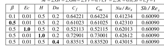
Table 2: Effect of various parameters on C_f ,

C

_m

,

Nu

/

Re

_x

,

and Sh/Re_xfor values of β,Ec,H Du, with

1 1 6 0 2 71 0 2 2

2 = = = = = = =

= ,Gr ,Gm ,Pr . ,F ,Sc . ,Sr ,γ M

β Ec H Du C_f C_m Nu/Re_x Sh/Re_x

0.1 0.01 0.5 0.2 0.64221 0.64224 0.41234 0.60090 0.5 0.01 0.5 0.2 0.61023 0.61025 0.42310 0.60090 0.5 1.0 0.5 0.2 0.52113 0.52115 0.62013 0.60090 0.5 0.01 1.0 0.2 0.72901 0.73001 0.42612 0.60090 0.5 0.01 0.5 0.4 0.83515 0.83520 0.43015 0.60090

Table 3: Effect of various parameters on C_f,C_m, Nu/Re_x, and Sh/Re_x for values of Sc, Sr,

γ

with

5 0 5 0 2 0 01 0 2 71 0 2 2

2,Gr ,Gm ,Pr . ,F ,Ec . ,Du . ,H . , .

M= = = = = = = = β=

Sc Sr γ C_f C_m Nu/Re_x Sh/Re_x

5. RESULTS AND DISCUSSIONS

The nonlinear boundary value problem solved in the previous section is dictated by an extensive number of thermal and hydrodynamic parameters. In order to gain a clear insight into the physical problem, numerical calculations for distribution of the velocity, microrotation (angular) velocity, temperature and concentration for different values of these parameters is conducted with graphical illustrations (Figs. 2-28). For the purpose of our computation, we adopted the following default parameters:ε=0.001, n=0.1,

t

=

1

,

A=0.5, B=0.1,E=0.1,β=0.2,

,

Gr=2 Gm=2, M=2, K=2, Pr=0.71, Sc=0.6,F=0.5,H=0.1, ,

.

Ec=001 Du=0.5,Sr=1.0,γ =1.0and all the graphs therefore correspond to these values, unless specifically indicated on the appropriate graph. The permeability in all the figures plotted is set at 0.5 which corresponds to a highly porous regime, characteristic of many materials operations and working MHD generators.The value of Pr is taken to be 0.71 which corresponds to air at 20°C and 1 atmospheric pressure and the value of Sc is 0.6 (water-vapour). Numerical values of the coefficient proportional to the skin friction C_f

, couple stress

coefficient Cm

, Nusselt number

Nu and Sherwood number Sh are given in Table 2 and Table 3 for the general model with all parameters invoked.

Analysis of the tabular data has been presented in Table 2 and Table 3. Table 2 depicts the effect ofβ,Ec,H,Duon C_f,C_m,Nu/Rexand

x Re /

Sh respectively. It is evident that both skin friction and wall couple stress decreases as β,Ecincreases while it increases as H,Duincreases. Further, it is observed that the Nusselt number decreases as Hincreases but it decreases as β,EcandDu increases. Sherwood number has no effect onβ,Ec,H,Du.Table 3, depicts the effect of Sc,Sr,γ on

x Re / Sh , x Re / Nu , m C , f

C respectively. The skin friction coefficient

decreases as Sc,Sr,γ increases. In case of wall couple stress same trend is observed. Further, Sherwood number increases as Sc,Sr,γincreases. But Nusselt number shows no variations on Sc,Sr,γ.

CPU took 6.52 seconds to compute the velocity and angular velocity profiles, 5.37 seconds to compute the temperature profiles, 4.96 seconds to compute the concentration profiles for 1001 nodal points with the Intel CORE i3 processor under windows platform, which are computed by using the Matlab command tic; {statements … …} toc;

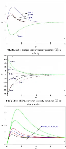
Figs 2 and 3 illustrate the influence of the Eringen vortex viscosity ratio parameter

( )

β on velocity and microrotation velocity profiles across the boundary layer. It is observed that the viscosity ratio less than 0.7 and fixed flow, the magnitude of the stream wise velocity increases and the inflection point for the velocity profiles moves farther away from the surface. The numerical results visualize the velocity of a Newtonian fluid

(

β=0

)

is lower as compared with a micropolar fluid one. When βtakes the values larger than 0.7, the flow near the porous plate decreases. The microrotation velocity profiles do not show consistent variations withβ. Figs 4 and 5 show the variations in velocity and microrotation velocity profiles for various values of thermal Grashof number,Gr. This parameter describes the relative magnitude of the buoyancy force and viscous force acting on the micropolar fluid. Grashof number

Gr

>

0

for cooling,

Gr

<

0

for heating and

Gr

=

0

implies absence of free convection currents. The velocity magnitudes are evidently enhanced for a vertical plate with an increase in thermal Grashof number. Momentum boundary layer thickness is therefore reduced. This is due to the dominance of buoyancy forces over the viscous forces, which in turn induce more flow and hence accelerates the fluid velocities. Furthermore, it is also noticed from the figure that the velocity starts with the velocity of the plate increases with a distance from the surface, reaches to maximum value in the vicinity of the plate, and decrease monotonically

to zero at the free stream. Conversely an increase in thermal Grashof number strongly damps the micro-rotation field i.e. decreases angular velocity of the micro-elements. Again values are consistently negative indicating a reverse spin in the micro-elements. As with linear velocity, in the free stream micro-rotation vanishes and is generally minimized at the plate.

Fig. 2 Effect of Eringen vortex viscosity parameter

( )

β

on velocity.

Fig. 3Effect of Eringen vortex viscosity parameter

( )

β

on micro-rotation.

Fig. 5 Effect of thermal Grashof number (Gr) on angular velocity

Figs 6 and 7 present the response in linear velocity and micro-rotation to a variation in species (solutal) Grashof number i.e. Gm. This parameter embodies the relative contribution of species buoyancy force to viscous hydrodynamic force. With increasing Gm, the mass diffusion effect leads to an acceleration in the flow i.e. increase in velocity values and an associated decrease in hydrodynamic boundary layer thickness. We note that for the case Gm = 0, species buoyancy effect vanishes and the momentum eqn. (16) is de-coupled from the species diffusion (concentration) eqn. (19). Micro-rotation values are significantly reduced with increasing Gm values i.e. increasing species buoyancy (associated with greater concentration gradient) exerts a similar influence to increasing thermal buoyancy and strongly damps the angular velocity. The spin of the micro-elements is therefore markedly inhibited with greater buoyancy effects.

Fig. 6 Effect of species (solutal) Grashof number (Gm) on velocity

Figs 8 and 9 show the pattern of the velocity and angular velocity for different values of magnetic field parameter M . It is observed that the amplitude of the velocity as well as the boundary layer thickness decreases when M is increased. Physically, it may also be expected due

to the fact that the magnetic field exerts a retarding effect on the free convective flow and upon increasing the values ofM , this type of

resisting force slows down the fluid, hence it is obvious that the effect of increasing values of the parameter M results in a decreasing velocity

distribution across the boundary layer. Similarly, in fig. 9 an increase in magnetic parameter is observed to significantly decelerate the angular velocity i.e. reduce the magnitude of micro-rotation, although the effect

from the plate. In both figs. 8 and 9 asymptotically smooth solutions are obtained indicating that a sufficiently large infinity boundary condition is prescribed in the free stream.

Fig. 7 Effect of species (solutal) Grashof number (Gm) on angular velocity.

Fig. 8 Effect of magnetic body force parameter (M) on velocity.

Fig. 9 Effect of magnetic body force parameter (M) on angular velocity.

medium. It arises in the Darcian drag force term in the composite linear momentum Eq. (16), viz −

(

1/ K

)

u. With increasing permeability, the regime solid fibers progressively decrease. The Darcian bulk impedance to flow is therefore also decreased. This results in acceleration in the velocity

u

, as observed in fig. 10. This behavior is sustained across the boundary layer i.e. for all values of transverse co-ordinate,

y

. It is also apparent that micro-rotation i.e. angular velocity is enhanced with greater permeability parameter although the effect is prominent near the plate surface and is weakened with further distance into the boundary layer. Since the permeability parameter does not arise in the angular momentum conservation (boundary layer) eqn. (17) the accelerating effect on micro-rotation is sustained via the boost in linear momentum experienced through the coupling terms which link both linear and angular momentum fields. The increase in permeability implies greater void space in the porous medium. This allows an enhancement in gyratory motions as the micro-elements are afforded greater space in which to spin.

Fig. 10 Effect of permeability parameter (K) on velocity.

Fig 11 Effect of permeability parameter (K) on angular velocity

Figs 12 and 13 illustrate the influence of Prandtl number (Pr) on the linear velocity and temperature profiles. With greater Prandtl number, it is observed in fig. 12, that the velocity is significantly decreased throughout the boundary layer. Prandtl number represents the relative rate of momentum diffusion to energy diffusion. With Pr > 1 the

momentum diffusion rate also exceeds the thermal diffusion rate in the fluid. Also fluids with higher Prandtl number possess greater viscosities and as Pr increases from 0.71 through 1, 2, to 5, the viscous resistance leads to depletion in velocity. This will also manifest in an increase in momentum (hydrodynamic) boundary layer thickness. Similarly, there is a strong depression in temperature with greater Prandtl number (Pr), greater Prandtl number corresponds to a lower thermal conductivity. This leads to a reduction in thermal energy convected through the fluid from the plate (Gr >0 i.e. plate cooling) and also depresses the thermal boundary layer thickness.

Fig. 12 Effect of Prandtl number (Pr) on velocity

Fig. 13 Effect of Prandtl number (Pr) on temperature

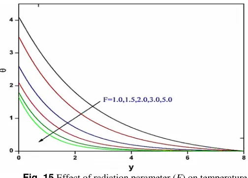
Fig. 15 Effect of radiation parameter (F) on temperature

Figs. 14 and 15 present the effect of thermal radiation-conduction parameter

( )

F on respectively linear velocity and temperature profiles. This parameter is defined as F=16

σ

T∞3

/

3kk and features in the augmented thermal diffusion term in eqn. (18) i.e.

₍

₎

2 2 1 1

y F

Pr ∂

∂

+ θ . This

parameter defines the relative contribution of thermal radiation heat transfer to thermal conduction heat transfer. When

F

>

1

thermal radiation dominates over thermal conduction, for

F

<

1

thermal conduction dominates. When

F

=

1

both thermal conduction and thermal radiation contributions are equal. For the present simulations, we confine attention to the case of

F

<

1

. Fig. 14 clearly reveals that there is a strong deceleration in the linear velocity with increasing F values. The energizing of the flow enhances thermal diffusion but counteracts momentum diffusion. This leads to an increase in momentum boundary layer thickness. A similar observation has been reported by Pal and Talukdar (2012). Increasing radiation-conduction parameter is also found to decrease temperatures in the boundary layer (fig. 15). Thermal boundary layer thickness is therefore also reduced with greater values of

F.

Fig. 16 Effect of heat absorption parameter

( )

H on velocity Figs. 16 and 17 depict the influence of heat generation parameter,

H, on velocity and temperature distribution, respectively in the flow. The heat absorption parameter Happearing in (18) quantifies the amount of heat absorbed per unit volume which is given byQ′

(

T_w′ −T_∞′

)

,Q′being a constant coefficient, which may take as either positive or negative or zero (no heat source/sink). The source term represents heat absorption

presence of heat absorption (thermal sink) effects has the tendency to reduce the fluid temperature. This de-energizes the flow and also causes a strong deceleration i.e. net reduction in the fluid velocity, as observed in Fig. 16. Greater heat absorption (H) clearly reduces the temperatures in the domain as observed in Fig. 17, and the effect is most prominent at the wall. Heat sources and sinks may therefore be utilized to great effect in materials processing systems and indeed can be introduced relatively easily in porous media.

Fig. 17 Effect of heat absorption parameter

( )

H on

temperature

Figs. 18 and 19 illustrate the influence of the Eckert number i.e. viscous dissipation parameter (Ec) on velocity and dimensionless temperature profiles.

Ec

expresses the relationship between the kinetic energy in the flow and the boundary layer enthalpy difference. It embodies the conversion of kinetic energy into internal energy by work done against the viscous fluid stresses. It is an important parameter for describing real working fluids in MHD energy generators and materials processing where dissipation effects are not trivial. Positive Eckert number corresponds to cooling of the wall (plate) and therefore a transfer of heat from the plate to the micropolar fluid. Convection is enhanced and we observe in consistency with that the fluid is accelerated i.e. linear velocity is increased in the micropolar fluid. Temperatures are also enhanced markedly with greater Eckert number, as shown in Figure 19 since internal energy is increased due to kinetic energy dissipation.

Fig 19 Effect of Eckert number (Ec) on temperature

Fig 20 Effect of Dufour number

( )

Du on velocity.

Fig 21 Effect of Dufour number

( )

Du on temperature

Figs. 20 and 21 depict the evolution in velocity and temperature function, respectively, with different values of diffuso-thermal parameter i.e. the Dufour number, _{mw / qw cs cp}

T K m D u

D = ν . The

Dufour effect refers to heat flux produced by a concentration (solutal) gradient. The fluid velocity increases with increase in Dufour number as seen in fig. 20. The augmented heat flux via the concentration field, therefore results in a thinning in the momentum boundary layer (acceleration). Increasing diffusion-thermo parameter (Du) also accentuates the temperature profiles as shown in Figure 21. The temperature profiles in the presence of the Dufour effect are higher in

comparison to in the absence of Dufour effect. The Dufour

cross-diffusion term, _

  

 

∂ ∂

+Du 2φ/ y2 in the energy (heat) conservation eqn.

(18) encourages diffusion of heat in the boundary layer via the solutal (concentration) gradient. The boundary layer flow is therefore energized with increasing Dufour number and thermal boundary layer thickness increases considerably in the presence of strong Dufour effects.

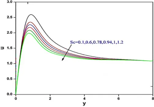
Fig 22 Effect of Schmidt number (Sc) on velocity.

Fig 23 Effect of Schmidt number (Sc) on concentration

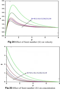
Fig 24 Effect of Soret number (Sr) on velocity

Fig 25 Effect of Soret number (Sr) on concentration

Figs. 24 and 25 present the effect of thermo-diffusive parameter i.e. Soret number which is defined as Sr = D_mK_T q_w /κ m_w ,on the translational velocity and concentration distributions, respectively. The Soret effect arises where small light molecules and large heavy molecules separate under a temperature gradient. Usually this effect is important where more than one chemical species is present under a very large temperature gradient such as CVD (chemical vapor deposition) in polymer materials processing, chemical reactors and energy generators. Figure 24 shows that a substantial elevation in velocity is induced with

increasing of

Sr

and therefore thermo-diffusion assists momentum development in the boundary layer, leading to a decrease in momentum boundary layer thickness. A marked enhancment in concentration profiles increases significantly with an increase of Soret numberSr. The Soret cross-diffusion term in the species conservation eqn. (19) i.e.

   

 

∂ ∂

+Sr 2θ/ y2 , encourages diffusion of solute in the boundary layer via

the thermal gradient. This results in a significant increase in concentration boundary layer thickness.

Figs. 26 and 27 illustrate the evolution in velocity and concentration with a change in chemical reaction parameter (γ). The reaction parameter is based on a first-order irreversible chemical reaction which takes place both in the bulk of the fluid (homogeneous) as well as at plate which is assumed to be catalytic to chemical reaction. Although chemical reactions generally fall into one of two categories i.e. homogenous or heterogenous, the former is of interest in the present study. Homogenous chemical reactions take place uniformly throughout a given phase and are similar in nature to an internal source of heat generation. We consider

values are found, in fig. 26, to instigate a considerable reduction in the velocity i.e. flow deceleration. The momentum boundary layer thickness is therefore also decreased substantially with greater chemical reaction effect. Fig. 27 shows that concentration is also depleted in the boundary layer with greater chemical reaction, since more species is destroyed via the chemical reaction. This results in a reduction in the thickness of the concentration boundary layer.

Fig 26 Effect of chemical reaction number (

γ

) on velocity

Fig 27 Effect of chemical reaction number (

γ

) on concentration

Fig 28 Comparison of fluid velocity with (Reddy, 2013).