A two-phase fuzzy programming model for a complex bi-objective no-wait flow shop scheduling Pages 617-626 Download PDF

(1)

Contents lists available at GrowingScience

International Journal of Industrial Engineering Computations

homepage: www.GrowingScience.com/ijiec

A two-phase fuzzy programming model for a complex bi-objective no-wait flow shop scheduling

Mahdi Naderi-Benia*, Reza Tavakkoli-Moghaddamb, Bahman Naderic, Ehsan Ghobadiana and Alireza Pourroustaa

a

Department of Industrial Engineering, Islamic Azad University, South Tehran Branch, Tehran, Iran

b

Department of Industrial Engineering, College of Engineering, University of Tehran, Tehran, Iran, Tehran, Iran

c

Young Researchers Club, Qazvin Branch, Islamic Azad University, Qazvin, Iran

A R T I C L E I N F O A B S T R A C T

Article history:

Received 25 January 2012 Accepted March, 5 2012 Available online 12 March 2012

In this paper, we study no-wait flow shop problem where setup times depend on sequence of operations. The proposed problem considers sequence-independent removal times, release date with an additional assumption that there are some preliminary setup times. There are two objectives of weighted mean tardiness and makespan associated with the proposed model of this paper. We formulate the resulted problem as a mixed integer programming, where a two-phase fuzzy programming is implemented to solve the model. To examine the performance of the proposed model, we generate several sample data, randomly and compare the results with other methods. The preliminary results indicate that the proposed two-phase model of this paper performed relatively better than Zimmerman's single-phase fuzzy method.

Keywords:

Flowshop No-wait Setup times Removal times bi-objective

Two phase fuzzy programming

1. Introduction

(2)

Wang et al. (2010) used accelerated Tabu search for NWFP problem for maximum lateness ( ). They increased the basic operations of generating better candidate solutions using Tabu search and reduced the complexity of the operations of NEH. Note that Hall et al. (1996) performed a comprehensive survey of scheduling problems with blocking and no-wait in process. There are many industries where setup times as well as processing times are independent from the operational times. Setup times include the necessary times for adding or exchanging equipments on facilities (Eren, 2009). Setup times and other related times are divided into two groups of independent and dependent times. There are many industrial cases where setup times depend on the operations such producing different colors using some common machines and the problem is called sequence-dependent setup time flow shop problem (SDSTFP).

Based on the notations developed by Graham et al. (1979), Allahvedi et al. (2008), Eren (2007),

different metaheuristics based on tabu search, random search for | | ∑ ∑

∑ ∑ have been developed. There are some mixed integer programming techniques,

which can be used to solve problems in small scales. For instance, Eren (2010) presented a mathematical programming to solve | | ∑ for relatively large-scale problems and gave three heuristics to solve the resulted problem. Mirabi (2010) presented a hybrid ant colony to solve | | . For a complete review of the literature, interested readers are referred to Allahverdi et al. (1999, 2008). Franca et al. (2006) proposed a genetic algorithm for | , ,

| and compared the performance of their method with Bianco et al. (1999).

Ruiz and Allahverdi (2007) investigated on SDSTFP problem in a form of | , | .

They investigated different heuristics as well as metaheuristics to solve the resulted problem and presented a dominance ratio for three-machine problem. Aldowaisan and Allahverdi (1998) provided a

solution methodology for | , | ∑ and presented one elimination criterion and

developed optimal solution for two special cases. Aldowaisan (2001) considered | , | ∑ problem one more time and tried to find a local and global dominance relations. In addition, they proposed some metaheuristics to solve the resulted problem, which seem to provide better quality solutions. They also used branch and bound method to provide a lower bound on this problem. Stafford and Tseng (2002) developed two models for family of flowshop sequencing problems of the form

| , | .

Gupta et al. (1997) provided a two-stage operations research models with setup and removal times separated. In their method, they considered setup times independent from operational times and proposed a method for minimizing makespan, which could be solved in polynomial time. Wang and Cheng (2006) proposed a heuristic approach for two-machine no-wait flowshop scheduling with due dates and class setups. They divided jobs to different groups with various setup times with an objective of minimizing the maximum lateness. The proposed model of this paper was developed for multi-objective problems. Jenabi et al. (2010) considered a bi-multi-objective NWFP problem. They first proposed two multi-objective mixed integer programming techniques and presented a local search to find efficient solutions. Javadi et al. (2008) presented fuzzy multi-objective problem for |

| , to find efficient solutions.

(3)

different areas of scheduling (Gharegozli et al., 2009; Tavakkoli-Moghaddam et al., 2010; Khademi-Zare & Fakhrzad, 2011).

In this paper, we present a multi-objective NWFP problem where the first objective is the minimization

of weighted average of lateness and the other objective is minimization of makespan. All setup times depend on the sequences of different jobs and machines. We also consider a preliminary setup time when the operations start, which is independent from the sequence of operations and only depends on the machines. The other assumption with the proposed model of this paper is that not all jobs are available at the beginning of the operations. In summary, the proposed model is denoted as

, , , , | , . There are literally many real-world applications where we can use the proposed model of this paper (Ruiz et al., 2008). The proposed model of this paper considers two objectives and it is formulated in a form of mixed integer programming and it is solved using the method proposed by Li et al. (2006). The organization of this paper first presents the mathematical model in section 2. The proposed solution methodology is given in section 3 and the performance of the proposed model is examined using different test problems and the results are given in section 4. Finally, concluding remarks are given in the last to summarize the contribution of the paper.

2. The proposed model

The proposed model of this paper considers , , , , , where IST is the

initial setup times for processing jobs located in the first stage of operations.

2.1 Assumptions

• All parameters are assumed deterministic.

• There must be no interruption when an operation starts on a particular machine.

• All jobs must precede the other operations on other machines as soon as they are finished with a particular machine unless the operations belong to the last machine.

• Each machine can only process one job at the same time.

• Processing times do not depend on sequence and they are all deterministic. • Not all jobs can be processed at the beginning of the operations.

• All machines are available in planning time horizon and there is no failure or interruption. • Removal time is independent from the processing and order of sequence and it is predefined.

Sets and indexes

J: Set of jobs 1,2, … , ; :

I: Set of machines 1,2, … , ; :

P: Set of positions 1,2, … , ; : ;

j,k: Job indexes , )

i: Machine indexes

p: Index of positions

Parameters

Weight of job

wj:

Release date for job

rj:

Due date of job

dj:

Processing time of job on machine

pji:

Removal time of job on machine

rtji:

Setup time of job on machine if it is processed immediately after job

sjik :

Initial setup time of job on machine if the job is in the first position of the sequence.

istji1:

Big number

(4)

Variables

Tardiness of job

Tj:

Maximum completion time

Cmax:

1 if job is in position

0 otherwise

j p

⎧ ⎨ ⎩

Xjp:

1 if job is processed right after job in position

0 otherwise

k j p

⎧ ⎨ ⎩

Yjkp:

The completion time of job on machine if it is in position in terms of sequence

Cjip:

The completion time of job on the last machine if it is in position in terms of sequence

Cjmp:

The earliest starting time of processing job on machine if it is in position

STjip:

The earliest starting time of processing job on the first machine if it is in position

STj1p:

The weighted mean lateness ∑ ∑_∑ :

2.2. The proposed bi-objective mixed integer programming (BMILP)

(1) min (2) min subject to: (3) ; ∑ 1 (4) ; ∑ 1 (5)

; , ; ; 2

(6)

; , ; ; 2

(7)

; ; 2

∑ ∑ 1

(8)

; , , .

(9)

; 1; , .

(10)

; , ; ; 2

1

(11)

; 1; , .

(12)

; 2; , .

(13)

; , ; ; 2

1 (14) ; , , (15) ; , , (16) ; , (17) ; , , (18) ; , 0,1 (19) ; , ; 0,1 (20) ; , ,

, , 0

(5)

shows the relationship between completion times of two sequential jobs. According to Eq. (14) and Eq. (15), we can make sure that if job in not in position then the earliest starting and completion times are equal to zero, otherwise, 1. Eq. (16) shows that makespan cannot be less than completion time of the last machine. Eq. (17) is also associated with the tardiness of job . Finally, Eqs. (18-20) show variable types definitions.

3. The proposed model

The proposed model of this paper uses a two-stage fuzzy programming, which is based on the method developed by Li et al. (2006) and the first stage uses Zimmerman's method (Zimmerman, 1978). We first present the necessary notations associated with the proposed model.

3.1. Notations

Satisfaction degree :

Satisfaction degree after the first stage

λ_ 1:

Satisfaction degree after the second stage

λ_ 2:

Satisfaction degree of the th

f objective function after the second stage 1,2

:

weight of satisfaction degree of the th

f objective function in the second stage 1,2 :

The lower bound of the first objective function :

The lower bound of the second objective function :

The value of the first objective function when the second objective function has the minimum

value z

:

The value of the second objective function when the first objective function has the minimum

value z

:

The value of the first objective function after the first stage terminates :

The value of the second objective function after the first stage terminates :

3.2 Solution procedure

3.2.1 Phase one

Step 1. The proposed BMILP is solved based on and the optimal value is called .

Step 2. Based on the solution obtained from the first step, is computed.

Step 3. The proposed BMILP is solved based on and the optimal value is called .

Step 4. Based on the solution obtained from the third step, is computed. Step 5. Solve the following linear programming problem.

(21)

max

subject to:

(22)

(23)

(24)

0,1

(25)

(6)

Step 6. Set λ_ 1 to computed λ in step 5.

3.2.2 Phase two

Step 7. Compute

و

based on the results of step 5 and store them in and , respectively. Solve the following linear programming problem,

(26)

max v λ v λ

subject to

(27)

(28)

(29)

(30)

(31)

1

(32)

, 0,1

(33)

Constraints (5-19)

Step 8. _ 2 is equal to optimal value obtained from Eq. (26) achieved from step 7.

Step 9. Repeat computations to calculate and until the final solutions are achieved.

4. Numerical examples

In order to measure the relative efficiency of the proposed model of this paper, we have solved 102 randomly generated test problems. Except and , which are determined by decision maker, all other values are predefined. Table 1 shows details of our input parameters.

Table 1

The method of generating input parameters

Parameters Values

The number of machines (m) 2,3,4

The number of jobs (n) 6,7,8

Processing time (pji) ~ 1,50

Release date (rj) ~ 0.100

Due date (dj)

∑ ∑ ∑ ∑ ∑ ∑ ∑ ∑ ∑

1

Weight (wj) ~ 1,10

Removal time (rtji) ~ 1,17

Setup time (sjik) ~ 1,17

Initial setup time (istji1) ~ 1,25

0.5

Total problem 3 3 5 45

(7)

In this section, we discuss the performance of the proposed model of this paper and compare the performance of two phase fuzzy method with Zimmerman's approach. We have solved all our test problems using LINGO-8 and the results are summarized in Table 2, Table 3 and Table 4.

Table 2

Results for 2-machine problems

Number of machines

Number of jobs

Number of

test λ of phase 1λ_PH1 λof phase 2λ_PH1

Objectives values of phase 1

T, C

Improvement in objectives

values

2 6 1 0.900 0.917 (33.533,305) (33.533,305) No

2 0.297 0.379 (65.476,314) (65.476,311) Yes

3 0.714 0.814 (52.963,302) (52.963,302) No

4 0.431 0.599 (71.792,331) (71.792,320) Yes

5 0.384 0.513 (72.844,334) (72.844,330) Yes

7 1 0.737 0.772 (59.342,358) (57.368,358) Yes

2 0.741 0.759 (60.089,295) (58.489,295) Yes

3 0.660 0.713 (64.65,343) (64.65,336) Yes

4 0.500 0.571 (74.586,416) (74.448,416) Yes

5 0.556 0.563 (63.407,351) (63.407,351) No

8 1 0.627 0.767 (70.830,459) (70.830,459) No

2 0.420 0.467 (60.830,420) (60.830,413) Yes

3 0.579 0.757 (85.587,398) (81.239,398) Yes

4 0.750 0.781 (58.745,348) (58.745,348) No

5 0.722 0.755 (44.789,363) (44.000,363) Yes

Table 3

Number of

machines Number of jobs Number of test λ of phase 1λ_PH1 λof phase 2λ_PH2 Objectives values of phase 1

T, C

values

3 6 1 0.533 0.594 (50.263,317) (43.688,317) Yes

2 0.755 0.801 (40.333,298) (40.333,296) Yes

3 0.475 0.593 (47.684,347) (43.895,347) Yes

4 0.465 0.625 (66.273,345) (66.273,340) Yes

5 0.579 0.640 (58.879,390) (58.879,390) No

7 1 0.551 0.627 (97.206,412) (82.5,412) Yes

2 0.778 0.836 (73.788,427) (73.788,418) Yes

3 0.428 0.507 (45.767,375) (45.767,367) Yes

4 0.555 0.635 (52.118,408) (52.118,404) Yes

5 0.243 0.312 (72.364,448) (72.364,442) Yes

8 1 0.475 0.679 (93.796,442) (93.796,435) Yes

2 0.404 0.450 (71.245,427) (68.981,427) Yes

3 0.384 0.387 (74.889,441) (74.889,440) Yes

4 0.750 0.817 (67.265,418) (67.265,418) No

5 0.772 0.781 (68.870,429) (68.870,427) Yes

Table 4

Number of machines

Number of jobs

Number of

test λ of phase 1λ_PH1 λof phase 2λ_PH1

T, C

values

4 6 1 0.324 0.638 (45.472,427) (45.672,400) Yes

2 0.243 0.590 (53.256,391) (53.256,368) Yes

3 0.557 0.716 (56.027,400) (56.027,387) Yes

4 0.696 0.765 (74.263,410) (74.263,408) Yes

5 0.533 0.535 (60.65,374) (60.65,374) No

7 1 0.625 0.653 (69.341,482) (69.431,480) Yes

2 0.704 0.736 (48.829,380) (48.829,377) Yes

3 0.571 0.620 (81.697,477) (74.485,477) Yes

4 0.545 0.547 (65.151,446) (65.151,445) Yes

5 0.500 0.613 (102.389,453) (102.389,453) No

8 1 0.909 0.942 (50.855,401) (49.873,401) Yes

2 0.612 0.682 (158.568,523) (88.864,523) Yes

3 0.130 0.322 (98.841,512) (96.884,512) Yes

4 0.393 0.562 (74.553,489) (72.319,489) Yes

(8)

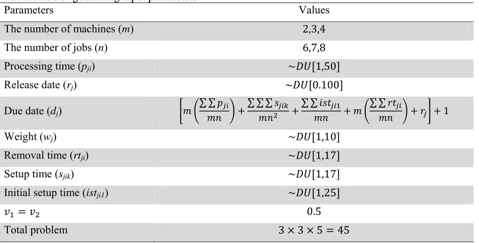
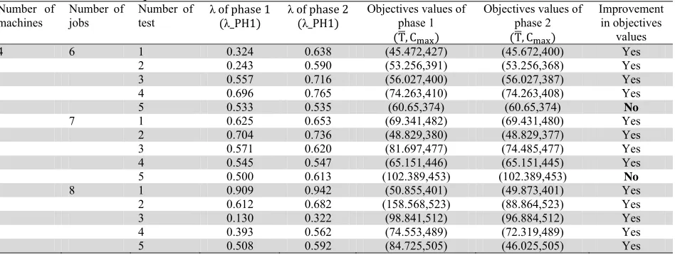
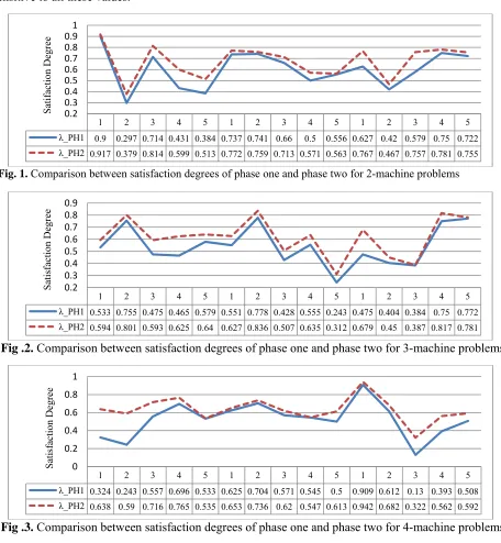
As we can observe from the results of Tables, the level of satisfaction degree of phase 2 is relatively better than the first level. In addition, Li et al. (2006) proved that the level of second level satisfaction will not be worse than the first level. Besides, 36 out of 45 sample test problems yields better results, which implies that the two-phase method performs better than the Zimmerman's method. Table 5 shows details of our results for different values of and . As we can observe the final solutions are sensitive to all these values.

Fig .2. Comparison between satisfaction degrees of phase one and phase two for 3-machine problems

Fig .3. Comparison between satisfaction degrees of phase one and phase two for 4-machine problems

5. Conclusions

In this paper, we have presented a no-wait flow shop problem where setup times depend on sequence of operations. The proposed problem considered sequence-independent removal times, release date with an additional assumption that there were some preliminary setup times. There were two objectives of weighted mean tardiness and makespan associated with the proposed model of this paper. The proposed model of this paper formulated the resulted problem as a mixed integer programming, where a two phase fuzzy programming was implemented to solve the model. To examine the performance of the proposed model, we have generated

1 2 3 4 5 1 2 3 4 5 1 2 3 4 5

λ_PH1 0.9 0.297 0.714 0.431 0.384 0.737 0.741 0.66 0.5 0.556 0.627 0.42 0.579 0.75 0.722

λ_PH2 0.917 0.379 0.814 0.599 0.513 0.772 0.759 0.713 0.571 0.563 0.767 0.467 0.757 0.781 0.755

0.2 0.3 0.4 0.5 0.6 0.7 0.8 0.9 1

Sa

ti

fact

ion De

gree

1 2 3 4 5 1 2 3 4 5 1 2 3 4 5

λ_PH1 0.533 0.755 0.475 0.465 0.579 0.551 0.778 0.428 0.555 0.243 0.475 0.404 0.384 0.75 0.772

λ_PH2 0.594 0.801 0.593 0.625 0.64 0.627 0.836 0.507 0.635 0.312 0.679 0.45 0.387 0.817 0.781

0.2 0.3 0.4 0.5 0.6 0.7 0.8 0.9

Sa

ti

sfa

ct

ion Degree

1 2 3 4 5 1 2 3 4 5 1 2 3 4 5

λ_PH1 0.324 0.243 0.557 0.696 0.533 0.625 0.704 0.571 0.545 0.5 0.909 0.612 0.13 0.393 0.508

λ_PH2 0.638 0.59 0.716 0.765 0.535 0.653 0.736 0.62 0.547 0.613 0.942 0.682 0.322 0.562 0.592

0 0.2 0.4 0.6 0.8 1

Sa

ti

sfa

ct

ion Degree

(9)

several sample data, randomly and compared the results with other methods. The results indicated that the proposed two-phase model of this paper performed relatively better than Zimmerman's single phase fuzzy method.

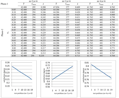
Table 5

The result of the implementation of the proposed 2-phase fuzzy programming with changing in value of

Phase-1 m=2,n=6 m=3,n=6 m=4,n=6

42.400 295 0.208 67.036 377 0.609 61.763 444 0.762

Ph

ase-2

0.05 42.400 294 0.248 64.286 377 0.614 61.763 441 0.804

0.10 42.400 294 0.246 64.286 377 0.620 61.763 441 0.802

0.15 42.400 294 0.244 64.286 377 0.625 61.763 441 0.800

0.20 42.400 294 0.242 64.286 377 0.631 61.763 441 0.798

0.25 42.400 294 0.240 64.286 377 0.636 61.763 441 0.795

0.30 42.400 294 0.237 64.286 377 0.642 61.763 441 0.793

0.35 42.400 294 0.235 64.286 377 0.647 61.763 441 0.791

0.40 42.400 294 0.233 64.286 377 0.653 61.763 441 0.789

0.45 42.400 294 0.231 64.286 377 0.658 61.763 441 0.786

0.50 42.400 294 0.229 64.286 377 0.664 61.763 441 0.784

0.55 42.400 294 0.227 64.286 377 0.669 61.763 441 0.782

0.60 42.400 294 0.225 64.286 377 0.675 61.763 441 0.780

0.65 42.400 294 0.223 64.286 377 0.680 61.763 441 0.778

0.70 42.400 294 0.221 64.286 377 0.686 61.763 441 0.775

0.75 42.400 294 0.219 64.286 377 0.691 61.763 441 0.773

0.80 42.400 294 0.217 64.286 377 0.697 61.763 441 0.771

0.85 42.400 294 0.215 64.286 377 0.702 61.763 441 0.769

0.90 42.400 294 0.212 64.286 377 0.708 61.763 441 0.767

0.95 42.400 294 0.210 64.286 377 0.713 61.763 441 0.764

Fig. 4. The impact of the changes in on satisfaction degree of phase two References

Aldowaisan, T., & Allahverdi, A. (1998). Total flowtime in no-wait flowshops with separated setup times.

Computers & Operation Research, 25, 757-765.

Aldowaisan, T. (2001). A new heuristic and dominance relations for no-wait flow shops with setups. Computers & Operations Research, 28, 563-584.

Allahverdi, A., Gupta, J.N.D., & Aldowaisan, T. (1999). A review of scheduling research involving setup considerations. Omega, The International Journal of Management science, 27, 219-239.

Allahvedi, A., Ng, C.T., Cheng, T.C.E., & Kovalyov, M.Y. (2008). A survey of scheduling problems with setups or costs. European Journal of Operational Research, 187, 985-1032.

Bianco, L., Dell’Olmo, P., & Giordani.S. (1999). Flowshop no-wait scheduling with sequence dependent setup times and release dates. INFOR, 37, 3-19.

Eren, T. (2007). A multicriteria flowshop scheduling problem with setup times. Journal of Materials Processing Technology, 186, 60-65.

0.19 0.2 0.21 0.22 0.23 0.24 0.25 0.26

1 4 7 10 13 16 19

satisf

action

deg

ree

test problem (m=2,n=6)

0.56 0.58 0.6 0.62 0.64 0.66 0.68 0.7 0.72 0.74

1 4 7 10 13 16 19

sati

sfacti

o

n

de

gr

ee

test problem (m=3,n=6)

0.74 0.75 0.76 0.77 0.78 0.79 0.8 0.81

1 4 7 10 13 16 19

sa

tisf

action

degree

(10)

Eren, T. (2009). A bicriteria parallel machine scheduling with a learning effect of setup and removal times.

Applied Mathematical Programming, 33, 1141-1150.

Eren, T. (2010). A bicriteria m-machine flowshop scheduling with sequence-dependent setup times. Applied Mathematical Programming, 34, 284-293.

Franca, P.M., Tin, Jr.G., & Buriol, L.S. (2006). Genetic algorithms for the no-wait flowshop sequencing problem with time restrictions. International Journal of Production Research, 44(5), 939-957.

Gharegozli, A.H., Tavakkoli-Moghaddam, R., & Zaerpour, N. (2009). A fuzzy-mixed-integer goal programming model for a parallel-machine scheduling problem with sequence-dependent setup times and release dates.

Robotics and Computers-Integrated Manufacturing, 25, 853-859.

Graham, R.L., Lawler, E.L., Lenstra, J.K., & Rinnooy Kan, A.H.G. (1979). Optimization and approximation in deterministic sequencing and scheduling: A survey. Annals of Discrete Mathematics, 5, 287-326.

Gupta, J.N.D., Strusevich, V.A., & Zwaneveld, C.M. (1997). Two-stage operations research models with setup and removal times separated. Computers & Operations Research, 24(11), 1025-1031.

Hall, N.G., & Sriskandarajah, C. (1996). A survey of scheduling problems with blocking and no-wait in process.

Operations Research, 44, 510-525.

Ishibuchi, H., Yamamoto, M., Misaki, S., & Tanaka, H. (1994). Local search algorithms for flow shop scheduling with fuzzy due-dates. International Journal of Production Economics, 33, 53-66.

Javadi, B., Saidi-Mehrabad, M., Haji, A., Mahdavi, I., Jolai, F., & Mahdavi-Amiri, N. (2008). No-wait flow shop scheduling using fuzzy multi-objective linear programming. Journal of Franklin Institute, 345, 452-467.

Jenabi, M., Naderi, B., & Ghomi, S.M.T.F. (2010). A bi-objective case of no-wait flowshops. IEEE, Changsha,

1048-1056.

Khademi-Zare, H., & Fakhrzad, M.B. (2011). Solving flexible flow-shop problem with a hybrid genetic algorithm and data mining: A fuzzy approach. Expert Systems with Applications, 38(6), 7609-7615.

Li, X.Q., Zhang, B., & Li, H. (2006). Computing efficient solutions to fuzzy multiple objective linear programming problems. Fuzzy Sets and Systems, 157, 1328-1332.

Liu, B., Wang, L., & Jin, Y.H. (2007). An effective hybrid particle swarm optimization for no-wait flow shop scheduling. International Journal of Advanced Manufacturing Technology, 31, 1001-1011.

Mirabi, M. (2010). Ant colony optimization technique for the sequence-dependent flowshop scheduling problem.

International Journal of Advanced Manufacturing Technology, 55(1-4), 317-326.

Pan, Q.K., Tasgetiren, M.F., & Liang, Y.C. (2008). A discrete particle swarm optimization algorithm for the no-wait flowshop scheduling problem. Computers & Operations Research, 35, 2807-2839.

Pinedo, M.L. (2008). Scheduling: Theory Algorithms and Systems. Third Edition, Springer.

Ruiz, R., & Allahverdi, A. (2007). No-wait flowshop with separated setup times to minimize maximum lateness. International Journal of Advanced Manufacturing Technology, 35, 551-565.

Ruiz, R., Serifoglu, F.S., & Urlings, T. (2008). Modeling realistic hybrid flexible flowshop scheduling problems.

Computer & Operations Research, 35, 1151-1175.

Stafford, E.F., & Tseng, F.T. (2002). Two models for family of flowshop sequencing problems. European Journal of Operational Research, 142, 282-293.

Tavakkoli-Moghaddam, R., Javadi, B., Jolai, F., & Ghodratnama, A. (2010). The use of a fuzzy multi-objective linear programming for solving a multi-objective single machine scheduling problem. Applied Soft Computing, 10, 919-925.

Tseng, L.Y., & Lin, Y.T. (2010). A hybrid genetic algorithm for no-wait flowshop scheduling problem. International Journal of Production Economics, 128, 144-152.

Wang, C., Li, X., & Wang, Q. (2010). Accelerated tabu search for no-wait flowshop scheduling problem with maximum lateness criterion. European Journal of Operational Research, 206, 64-72.

Wang, X., & Cheng, T.C.E. (2006). A heuristic approach for two-machine no-wait flowshop scheduling with due dates and class setups. Computers & Operations Research, 33, 1326-1344.

Wu, H.C. (2010). Solving the fuzzy earliness and tardiness in scheduling problems by using genetic algorithms.

Expert Systems with Applications, 37, 4860-4866.

Yao, J.S., & Feng, T.S. (2002). Constructing a fuzzy flow-shop sequencing model based on statistical data.

International Journal of Approximate Reasoning, 29, 215-234.

Zimmerman.H.J., (1978), Fuzzy programming with several objective functions, Fuzzy Sets and Systems, 1,