Vol. 7, No. 3, 2015 Article ID IJIM-00647, 8 pages Research Article
Two new three and four parametric with memory methods for solving
nonlinear equations
T. Lotfi ∗†, P. Assari ‡
————————————————————————————————–
Abstract
In this study, based on the optimal free derivative without memory methods proposed by Cordero et al. [A. Cordero, J.L. Hueso, E. Martinez, J.R. Torregrosa, Generating optimal derivative free iterative methods for nonlinear equations by using polynomial interpolation, Mathematical and Computer Modeling. 57 (2013) 1950-1956], we develop two new iterative with memory methods for solving a nonlinear equation. The first has two steps with three self-accelerating parameters, and the second has three steps with four self-accelerating parameters. These parameters are calculated using information from the current and previous iteration so that the presented methods may be regarded as the with memory methods. The self-accelerating parameters are computed applying Newton’s interpolatory polynomials. Moreover, they use three and four functional evaluations per iteration and corresponding R-orders of convergence are increased from 4 ad 8 to 7.53 and 15.51, respectively. It means that, without any new function calculations, we can improve convergence order by 93% and 96%. We provide rigorous theories along with some numerical test problems to confirm theoretical results and high computational efficiency.
Keywords : Nonlinear equation; With memory method; R-order of convergence; Self accelerating parameter; Efficiency index.
—————————————————————————————————–
1
Introduction
M
uory methods for solving a nonlinear equa-lti-point iterative with and without mem-tion are great importance among the researchers in this field. Without doubt, Traub [14] and Os-trowski [12] made major contributions. Kung and Traub conjectured any optimal multi-point with-out memory method has convergence order 2n us-ing exactly n+ 1 functional evaluations per full cycle [4].In addition, Ostrowski introduced a criteria for
∗Corresponding author. [email protected]
†Department of Mathematics, Hamedan Branch, Is-lamic Azad University, Hamedan, Iran.
‡Department of Mathematics, Hamedan Branch, Is-lamic Azad University, Hamedan, Iran.
comparing different methods, say, efficiency in-dex which is defined byEI =p1n, wherep and n represent convergence order and functional eval-uations, respectively.
Based on Kung and Traub’s conjecture, during the last two decades many researchers have de-signed many optimal without memory methods [1,5,17] and over recent years several with mem-ory methods have presented [2,3] and [6-11], too. In this study, we consider two kind of Cordero et al.’s methods [1] and try to develop two new with memory methods. Our improvements have not been studied before. As the main contribu-tion of this work, convergence orders have been increased from 4 and 8 to 7.53 and 15.51, respec-tively, without any new functional evaluations. First, we modify the first two and three steps of
Cordero et al.’s method [1] in such a way that they are still optimal. Then, introducing the best approximations for considered accelerators, we attempt to derive our new with memory meth-ods.
The rest of this paper is organized as follows: Sec-tion 2is devoted to modifications of the two and three steps of Cordero et al.’s methods [1]. Sec-tion3concerns with developing new with memory methods. Section4includes some numerical per-formances. And, Section 5 comprises conclusion remarks.
2
Modified
three-
and
Four-parametric methods
2.1 three-parametric two-point method
In this section, our goal is to modify two opti-mal without memory methods by Cordero et al. [1]. Let start by the following optimal two-point without memory method
zn=xn−
f(xn)
f[xn, wn]
,
xn+1 =zn−
f(zn)
p′2(zn)
,
(2.1)
with this error equation
en+1 = (1 +f′(α))2c2(c22−c3)e4n+O(e5n). (2.2)
Where wn = xn + f(xn), and p2(zn) is the interpolating polynomial of the points (xn, f(xn)),(wn, f(wn)), (zn, f(zn)). This poly-nomial can be written as
p2(x) = xxnn−−wznnf[wn, zn] +wwnn−−zxnnf[xn, zn], (2.3)
so, we have
p′2(zn) =f[xn, zn]−f[xn, wn] +f[wn, zn]. (2.4)
Now, we consider the following modification of (2.1) by adding three free parametersγ,p, andλ
wn=xn+γf(xn),
zn=xn−
f(xn)
f[xn, wn] +pf(wn)
,
xn+1 =zn−
f(zn)
p′2(zn) +λ(zn−xn)(zn−wn)
.
(2.5) This method is of four convergence order and we state it formally in the following theorem
Theorem 2.1 Let f :D→R be sufficiently dif-ferentiable function with a simple root α ∈ D,
D ⊂R be an open set, x0 be close enough to α, then the method (2.5) is at least of fourth-order, and satisfies α the error equation
en+1 = (1+γf
′(α))2(p+c
2)(λ+c2f′(α)(p+c2)−c3f′(α))e4n f′(α)
+O(e5n), (2.6)
where en=xn−α andcj = f
(j)(α)
j!f′(α).
Proof. We use the Mathematica for finding the error equation.
f[e ] =f1a∗(e+∑4k=2ck∗ek
)
;
ew=e+'f[e] (∗ew=w−α∗);
f[x ,y ] := f[xx]−−fy[y];
ez=e−Series[f[e,ewf]+[e]pf[ew],{e,0,4}] (∗ez=z−α∗)
Out[a] : (1+ f1a')(p+c2)e2+O[e]3.
p2[t] =a0+a1(t−ez) +a2(t−ez)2;
dp2[t] :=a1+2a2(t−ez);
a1:=f[e,ez]−f[e,ew] +f[ew,ez];
en+1 =ez−
f[ez]
dp2[ez]+˘(ez−e)(ez−ew)//Simplify;
Out[b] : (1+f1a')2(p+c2)(˘+c2f1a(p+c2)−c3f1a)e4
f1a +O[e]5.
Therefore, we have
en+1 = (1+γf
′(α))2(p+c
2)(λ+c2f′(α)(p+c2)−c3f′(α))e4n f′(α)
+O(e5n).
2.2 Four-parameteric three-point method
Now, we consider the following optimal three-point without memory method that has proposed by Cordero et al. [1]
zn=xn−
f(xn)
f[xn, wn]
,
un=zn−
f(zn)
p′2(zn)
, n= 0,1,· · ·,
xn+1 =un−
f(un)
p′3(un)
,
(2.7)
with this error equation
en+1 = (1 +f′(α))4c22(c22−c3)
(c32−c2c3+c4)e8n+O(e9n). (2.8)
(un, f(un)). This polynomial can be written as
p3(x) = ((xxn−n−wun)(n)(zzn−n−uwn)n)f[wn, un]
+((wwn−n−xun)(n)(zzn−n−uxn)n)f[xn, un] (2.9)
+(wn−un)(xn−un)
(wn−zn)(xn−zn)f[zn, un], so, we have
p′3(un) =−
(
f[zn, un](wn−un)(xn−un)
(xn−wn) +f[xn, un](wn−un)
(zn−un)(wn−zn) +f[wn, un]
(xn−un)(zn−un)(zn−xn)
)
/
(
(xn−un)((wn−un)(1−xn−zn
+ 2un) + (xn−un)(zn−un))
)
.
(2.10)
Then, we modify (2.7) as follows similar to (2.5)
wn=xn+γf(xn),
zn=xn−f[xn,wfn]+(xn)pf(wn),
un=zn−p′ f(zn)
2(zn)+λ(zn−xn)(zn−wn),
xn+1=un−p′ f(un)
3(un)+β(un−wn)(un−xn)(un−zn).
(2.11) This method is of eight convergence order and we demonstrate it officially in the following theorem
Theorem 2.2 Let f :D→R be sufficiently dif-ferentiable function with a simple root α ∈ D,
D ⊂R be an open set, x0 be close enough to α, then the method (2.11) is at least of eighth-order, and satisfies α the error equation
en+1 = (
1 +γf′(α))4(p+c2)2(λ+c2f′(α)
(p+c2)−c3f(α))(−β+c2(λ+c2f′(α)
(p+c2)−c3f′(α)) +c4f′(α))e8n
)
f′(α)2
+O(e9n), (2.12)
where en=xn−α and cj = f
(j)(α)
j!f′(α).
Proof. We use the Mathematica for finding the error equation.
f[e ] =f1a∗(e+∑5k=2ck∗ek
)
;
ew=e+'f[e] (∗ew=w−α∗);
f[x ,y] := f[xx]−−fy[y];
ez=e−Series[f[e,ewf]+[e]pf[ew],{e,0,8}]
(∗ez=z−α∗)
Out[a] : (1+ f1a')(p+c2)e2+O[e]3.
p2[t ] =a0+a1(t−ez) +a2(t−ez)2;
dp2[t ] :=a1+2a2(t−ez);
a1:=f[e,ez]−f[e,ew] +f[ew,ez];
eu=ez−dp f[ez]
2[ez]+˘(ez−e)(ez−ew)//Simplify
(∗eu=u−α∗)
Out[b] : (1+f1a')2(p+c2)(˘+c2f1a(p+c2)−c3f1a)e4
f1a +O[e]5.
p3[t ] =b0+b1(t−eu) +b2(t−eu)2 +b3(t−eu)3;
dp3[t ] :=b1+2b2(t−eu) +3b3(t−eu)2;
b1:=−
(
f[ez,eu](ew−eu)(e−eu)(e−ew) +f[e,eu](ew−eu)(ew−eu)(ew−ez)
+f[ew,eu](e−eu)(ez−eu)(ez−e)
)
/
(
(e−eu)((ew−eu)(1−e−ez
+2eu) + (e−eu)(ez−eu))
)
;
en+1 =eu−dp3[eu]+↓(eu−few[eu)(]eu−e)(eu−ez)
Out[c] :
(
(1+f1a')4(p+c
2)2(˘+c2f1a (p+c2)−c3f1a)(−↓+c2(˘+c2f1a
(p+c2)−c3f1a) +c4f1a)e8
)
/f1a2
+O[e]9.
Therefore, we gain
en+1 = (
(1 +γf′(α))4(p+c2)2(λ+c2f′(α)
(p+c2)−c3f′(α))(−β+c2(λ
+c2f′(α)(p+c2)−c3f′(α))
+c4f′(α))e8n
)
/f′(α)2+O(e9n).
3
The
developments
of
new
with memory methods
3.1 A new family of two-step with memory methods
to increase convergence order, we consider
1 +γnf′(α) = 0,
pn+c2= 0,
λn+f′(α)c2(p+c2)−f′(α)c3= 0,
(3.13)
So, we have
γn=−f′1(α), pn=−f ′′(α)
2!f′(α), λn= f′′′(α)
3! . (3.14)
Becauseαis unknown, therefore, we can not com-pute f(J)(α), j = 1,2,3. Then, we use interpola-tion to approximate them as follows
γn=−N′1
3(xn), pn=−
N4′′(wn)
2!N4′(wn), λn= f5′′′(zn)
3! ,
whereN3(t) andN4(t) are Newton’s iterpolatory polynomials of third and fourth degrees. Hence, the new with memory method is given by
x0, γ0, p0 are given, then w0=x0+γ0f(x0),
γn=−N′1
3(xn), pn=−
N4′′(wn)
2N4′(wn), λn= f5′′′(zn)
3! ,
wn=xn+γnf(xn),
zn=xn−f[xn,wn]+f(xn)pnf(wn), n= 1,2,· · ·,
xn+1 =zn−p′ f(zn)
2(zn)+λn(zn−xn)(zn−wn).
(3.15) To prove its convergence order, we need to fol-lowing lemma
Lemma 3.1 If γn = −1/N3′(xn) and pn =
−N4′′(wn)/(2N4′(wn)), n = 1,2, . . ., then the es-timates
1 +γnf′(α)∼en−1,zen−1,wen−1, (3.16)
and
c2+pn∼en−1,zen−1,wen−1, (3.17)
and
λn+f′(α)c2(pn+c2)−f′(α)c3
∼en−1,zen−1,wen−1, (3.18)
hold.
Proof. Similar to Lemma 1 in [15] and Lemma 4 and 6 in [9].
The following theorem determines the conver-gence order of the two-point iterative with mem-ory method (3.15).
Theorem 3.1 If an initial estimationx0 is close enough to a simple root α of f(x) = 0, being f
a real sufficiently differentiable function, then the
R-order of convergence of the two-point method with memory (3.15) is at least 7.5311.
Proof. Let{xn} have converged orderR. Then, we can write
en+1∼eRn, en=xn−α, (3.19)
Hence
en+1∼eRn = (eRn−1)R=eR
2
n−1. (3.20)
Suppose sequences{wn}and{yn}have converged
p and q, respectively,
en,w ∼epn= (eRn−1)p =e Rp
n−1 (3.21)
and
en,z ∼eqn= (eRn−1)q =e Rq
n−1. (3.22)
By (3.22), (3.21), and Lemma 3.1, we obtain
1 +γnf′(α)∼epn+−q1+1, (3.23)
c2+pn∼epn+−q1+1. (3.24)
Substituting these into en,w, en,y, and en+1 in Theorem3.1, we have
en,w ∼
(
1 +γnf′(α)
)
en=e(1+n−1p+q)+R, (3.25)
en,z ∼c2 (
1 +γnf′(α)
)
(c2+pn)e2n
=e2(1+n−1p+q)+2R, (3.26)
and
en+1∼A4 (
1 +γnf′(α)
)2
(c2+pn)
(λ+f′(α)c2(p+c2)−f′(α)c3)e4n
∼e4(1+n−1p+q)+4R. (3.27)
Equating the powers of error exponents ofen−1in pairs of relations (3.21)-(3.25), (3.22)-(3.26), and (3.20)-(3.27), we have
Rp−R−(p+q+ 1) = 0, Rq−2R−2(p+q+ 1) = 0,
R2−4R−4(p+q+ 1) = 0.
(3.28)
This system has the solution p = 1.8828, q = 3.7656, and R = 7.5311 which specifies the R-order of convergence of the derivative-free scheme
3.2 A new family of three-step with memory methods
In a similar way to former section, in addi-tion to menaddi-tioned parameters, due to three-point method error equation (2.12), we modifyβ →βn, too. Then, we have
1 +γnf′(α) = 0,
pn+c2 = 0,
λn+f′(α)c2(p+c2)−f′(α)c3 = 0, −βn+c2(λ+c2f′(α)(p+c2)−c3f′(α)) +c4f′(α) = 0.
(3.29) So, we gain
γn=−f′1(α), pn=−f ′′(α) 2!f′(α),
λn= f ′′′(α)
3! , βn=
f(4)(α)
4! . (3.30)
Becauseαis unknown, therefore, we can not com-putef(J)(α), j = 1,2,3,4. Then, we use interpo-lation to approximate them as follows
γn=−N′1
4(xn), pn=−
N5′′(wn) 2!N5′(wn),
λn= N ′′′
6 (zn)
3! , βn=
N7(4)(un) 4! ,
where Ni(t),(i= 4,5,6,7), are Newton’s iterpo-latory polynomials of i degrees. As we state in previous section by estimating γn, pn, λn, and
βn with Newton’s interpolatory polynomials, we find out new three-point methods with memory as follows
x0, γ0, p0 are given, then w0=x0+γ0f(x0),
γn=−N′1
4(xn), pn=−
N5′′(wn) 2N5′(wn),
wn=xn+γnf(xn), n= 1,2, . . . ,
zn=xn−f[xn,wfn]+(xn)pnf(wn),
un=zn−p′ f(zn)
2(zn)+λn(zn−xn)(zn−wn),
xn+1 =un−p′ f(un)
3(un)+βn(un−wn)(un−xn)(un−zn).
(3.31) To demonstrate the convergence order of (3.31), we require this lemma
Lemma 3.2 If γn = −1/N4′(xn) and pn =
−N5′′(wn)/(2N5′(wn)), n = 1,2, . . ., then the
es-timates
1 +γnf′(α)∼en−1,uen−1,zen−1,wen−1, (3.32)
and
c2+pn∼en−1,uen−1,zen−1,wen−1, (3.33)
λn+f′(α)c2(pn+c2)−f′(α)c3
∼en−1,uen−1,zen−1,wen−1, (3.34) −β+c2(λ+c2f′(α)(p+c2)−c3f′(α))
+c4f′(α)∼en−1,uen−1,zen−1,wen−1, (3.35)
hold.
Proof. Similar to Lemma 1 in [15] and Lemma 4 and 6 in [9].
The next theorem shows that the convergence order of the three-step iterative with memory method (3.31).
Theorem 3.2 If an initial estimationx0 is close enough to a simple root α of f(x) = 0, being f
a real sufficiently differentiable function, then the
R-order of convergence of the three-step method with memory (3.31) is at least 15.5156.
Proof. Let{xn} have converged orderR. Then, we can write
en+1∼eRn, en=xn−α, (3.36)
Hence
en+1∼eRn = (eRn−1)R=eR
2
n−1. (3.37)
Assume sequences {wn}, {zn}, and {un} have convergedp,q, and s, respectively, that is
en,w ∼epn= (eRn−1)p=e Rp
n−1, (3.38)
en,z ∼eqn= (eRn−1)q =e Rq
n−1, (3.39)
and
en,u∼esn= (eRn−1)s=eRsn−1. (3.40)
By (3.38), (3.39), (3.40), and Lemma3.2, we ob-tain
1 +γnf′(α)∼enp+−q1+s+1, (3.41)
c2+pn∼enp+−q1+s+1. (3.42)
Substituting these into en,w, en,z, en,u, and en+1 in Theorem3.2, we have
en,w ∼
(
1 +γnf′(α)
)
Table 1: Computational order of convergence of (3.31)
functions |x1−α| |x2−α| |x3−α| COC
f1(x) 8.2290(−3) 1.0503(−30) 1.4474(−472) 15.848 f2(x) 1.2212(−2) 7.8503(−36) 1.9533(−549) 15.475 f3(x) 3.3663(−3) 5.6416(−46) 1.6379(−713) 15.605 f4(x) 6.2164(−4) 7.3597(−43) 1.3871(−652) 15.664 f5(x) 2.8111(−7) 9.0115(−107) 8.5433(−1644) 15.448
Table 2: Computational order of convergence of (3.15)
functions |x1−α| |x2−α| |x3−α| COC
f1(x) 1.0831(−2) 1.1281(−13) 2.1218(−99) 7.7936 f2(x) 4.6845(−2) 3.0552(−10) 2.1117(−74) 7.8469 f3(x) 1.1972(−2) 4.8007(−19) 8.2100(−142) 7.4840 f4(x) 1.4378(−3) 7.6488(−12) 4.8261(−85) 8.8502 f5(x) 4.5624(−4) 3.6324(−26) 1.3751(−192) 7.5307
en,z ∼c2 (
1 +γnf′(α)
)
(c2+pn)e2n
=e2(1+n−1p+q+s)+2R, (3.44)
en,u∼an,4 (
1 +γnf′(α)
)2
(c2+pn)
(λ+f′(α)c2(p+c2)−f′(α)c3)e4n
=e4(1+n−1p+q+s)+4R, (3.45)
and
en+1∼an,8 (
1 +γnf′(α)
)4
(c2+pn)2(λ+f′(α)c2
(p+c2)−f′(α)c3)(−β+c2(λ+c2f′(α)
(p+c2)−c3f′(α)) +c4f′(α))e8n
∼e8(1+n−1p+q+s)+8R. (3.46) Equating the powers of error exponents of en−1 in pairs of relations (3.38)-(3.43), (3.39)-(3.44), (3.40)-(3.45), and (3.37)-(3.46), we have
Rp−R−(p+q+s+ 1) = 0,
Rq−2R−2(p+q+s+ 1) = 0, Rs−4R−4(p+q+s+ 1) = 0, R2−8R−8(p+q+s+ 1) = 0.
(3.47)
This system has the solution p = 1.9394, q = 3.8789, s= 7.7578, andR= 15.5156 which spec-ifies the R-order of convergence of the derivative-free scheme with memory (3.31). 2
4
Numerical Results
Now we show the convergence behavior of de-veloped the with memory methods in action. For
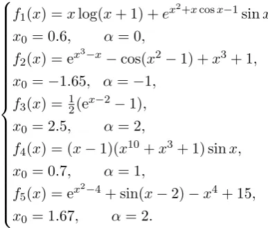
this purpose, ten test problems are chosen along with their initial approximations and the exact zeros in Table 1. The errors |xn − α| denote approximations to the sought zeros, and a(−b) stands for a×10−b. Moreover, COC indicates the computational order of convergence [16] and is computed by
COC = log|f(xn)/f(xn−1)| log|f(xn−1)/f(xn−2)|
. (4.48)
To carry out the numerical results, the pack-age Mathematica 9 with multi-precision arith-metic was used. We have used γ0 = 0.01, p0 = −1, λ0 = 0.1, β0 = 5 for all test problems. In Tables1 and2, we have examined some methods with different kinds of convergence order. It is observed that these methods support their theo-retical aspects.
f1(x) =xlog(x+ 1) +ex
2+xcosx−1
sinx, x0 = 0.6, α= 0,
f2(x) = ex
3−x
−cos(x2−1) +x3+ 1, x0 =−1.65, α=−1,
f3(x) = 12(ex−2−1),
x0 = 2.5, α= 2,
f4(x) = (x−1)(x10+x3+ 1) sinx,
x0 = 0.7, α= 1,
f5(x) = ex
2−4
5
Conclusion
In this work, we have improved two kinds of optimal without memory methods so that they achieve convergence orders 7.53 and 15.51, re-spectively, using three and four functional eval-uations. In other words, the efficiency indices of the optimal without memory methods have been increased from 413 ≃ 1.5874 and 8
1
4 ≃ 1.6818
to 7.5313 ≃ 1.9600 and 15.51 1
4 ≃ 1.9845, which
means that we were able to increase the conver-gence orders about 93% and 96%, respectively. Studying basin of attractions of the proposed methods can be considered for the future works.
References
[1] A. Cordero, J. L. Hueso, E. Martinez, J. R. Torregrosa,Generating optimal derivative free iterative methods for nonlinear equations by using polynomial interpolation, Mathe-matical and Computer Modelling 57 (2013) 19501956.
[2] A. Cordero, T. Lotfi, J. R. Torregrosa, P. As-sari, K. Mahdiani, Some new bi-accelerator two-point methods for solving nonlinear equations, Comp. Appl. Math. http://dx. doi.org/10.1007/s40314-014-0192-1.
[3] A. Cordero, T. Lotfi, P. Bakhtiari, J. R. Tor-regrosa, An efficient two-parametric family with memory for nonlinear equations, Nu-mer Algor. http://dx.doi.org/10.1007/ s11075-014-9846-8.
[4] H. T. Kung, J. F. Traub, Optimal order of one-point and multipoint iteration, J. Assoc. Comput. Math. 21 (1974) 634-651.
[5] T. Lotfi, A new optimal method of fourth-order convergence for solving nonlinear equations, International Journal of Indus-trial Mathematics 6 (2014) 121-124.
[6] T. Lotfi, P. Assari, A new calss of two step methods with memory for solving nonlinear equation with high efficiency index, Inter-national Journal of Mathematical Modelling and Computations 4 (2014) 277-288.
[7] T. Lotfi, K. Mahdiani, Z. Noori, F. Khak-sar Haghani, S. Shateyi, On a new three-step class of methods and its acceleration
for nonlinear equations, The Scientific World Journal. Volume 2014, Article ID 134673, 9 pages.
[8] T. Lotfi, S. Shateyi, S. Hadadi, Potra-Pt´ak iterative method with memory, ISRN Math-ematical Analysis. Volume 2014, Article ID 697642, 6 pages.
[9] T. Lotfi, F. Soleymani, Z. Noori, A. Kili-man, F. Khaksar Haghani, Efficient itera-tive methods with and without memory pos-sessing high efficiency indices, Discrete Dy-namics in Nature and Society. Volume 2014, Article ID 912796, 9 pages.
[10] T. Lotfi, F. Soleymani, S. Shateyi, P. Assari, F. Khaksar Haghani, New mono- and biac-celerator iterative methods with memory for nonlinear equations, Abstract and Applied Analysis. Volume 2014, Article ID 705674, 8 pages.
[11] T. Lotfi, E. Tavakoli,On construction a new efficient Steffensen-like iterative class by ap-plying a suitable self-accelerator parameter, The Scientific World Journal. Volume 2014, Article ID 769758, 9 pages.
[12] A. M. Ostrowski, Solution of Equations and Systems of Equations, Academic Press, New York, 1960.
[13] J. F. Steffensen, Remarks on iteration, Skand. Aktuarietidskr 16 (1933) 64-72.
[14] J. F. Traub, Iterative Methods for the Solu-tion of EquaSolu-tions, Prentice Hall, New York, 1964.
[15] X. Wang, T. Zhang, A new family of Newton-type iterative methods with and without memory for solving nonlinear equa-tions, Calcolo. http://dx.doi.org/10. 1007/s10092-012-0072-2.
[16] S. Weerakoon, T. G. I. Fernando, A variant of Newton’s method with accelerated third-order convergence, J. Appl. Math. Lett. 13 (2000) 87-93.
Taher Lotfi has got MSc de-grees in Applied Mathematics from Kharazmi (Tarbiat Moallem) Uni-versity, and PhD degree from Sci-ence and Research Branch, Islamic Azad University, Tehran, Iran. My main research interests include ap-proximating numerical solutions using iterative methods for nonlinear systems of equations, spe-cially for large systems arising from IE, ODE and PDE. Also, interval analysis, reproducing kernel space methods, soft computing based on wavelets and fuzzy concepts, generalized inverses are my current MSc and PhD students research field.