Computational Procedure for Calculating Sherwood Number Values in Vertical Channel Geometry by using the Numerical Method Finite Element Method

(1)

Computational Procedure for Calculating

Sherwood Number Values in Vertical Channel

Geometry by using the Numerical Method

Finite Element Method

P. Reddaiah

#1

D.R.V. Prasada Rao

*2

#_{Professor of Mathematics, Global College of Engineering and Technology, kadapa, Andhra Pradesh, India.}

*Professor of Mathematics, Sri Krishnadevaraya University, Anantapur, Andhra Pradesh, India.

Abstract — In this paper we analyzed the computational procedure for calculating Sherwood number values by Mathematica 4.1 Software Commands in Vertical Channel Geometry by using the Numerical Method Finite Element Method (FEM).

Keywords — Sherwood number, Vertical Channel,

Finite Element Method.

I.INTRODUCTION

Natural convection, a passive mode of heat transfer, is considered to be a promising option for cooling of electronic components in air because of the specific features of natural convection such as simplicity in design, low installation and maintenance cost, reliability and noiseless operation. Natural convection from protruding and flush mounted heat generating elements has received considerable attention in heat transfer literature, as they simulate heat generating electronic components such as resistors, capacitors, inductors, transformers, ICs and so on. Mixed convection flow through a heated channel has been extensively explored because of its occurrence in many practical applications such as the cooling of modern electronic systems, heat exchangers, solar energy collection, as in the conventional flat plate collector, chemical processing equipment’s, transport of heated or cooled fluids, etc.

Barletta et al [1] studied the Combined Forced and Free Convective Flow in a Vertical Porous Channel: The Effects of Viscous Dissipation and Pressure Work. Nadeem et al [2] studied the Magneto hydrodynamic peristaltic flow of a hyperbolic tangent fluid in a vertical asymmetric channel with heat transfer.

Fig.a: Schematic diagram of the Vertical Channel

Nomenclature u Velocity T Temperature C Concentration p Pressure

 Density

 Coefficient of Kinematic viscosity K Permeability Coefficient k1 Coefficient of thermal

conductivity

o Mean density

To Mean temperature

Co Mean Concentration

Cp Specific heat at constant pressure  Coefficeint of thermal expansion

*_{Volumetric Coefficient of}

expansion with mass fraction concentration



Q Strength of the heat source D1 Molecular Diffusivity

K11 Cross diffusivity

II. Formulation of the Problem

(2)

account in the energy equation as the modification of the heat flow. The fluid and the porous matrix are in local thermal equilibrium and the flow is unidirectional along the direction of the buoyancy.

We choose the Cartesian frame of reference 0 (x, y, z) such that the x-axis is in upward vertical direction against buoyancy and the vertical walls are parallel to (y, z) plane y =  b (Fig .a). Let (u, 0, 0) be the velocity field of the unidirectional flow along the channel and T the temperature in the flow field and to the ambient temperature. The equations governing the flow, heat and mass transfer with soret and dissipative effects are

0 (1)

u x    2 2

( ₂ ₂ ) ( ₀)

*₍ ₎

0 (2)

u u u

g T T

k

y z

u

g C _{C o} v

y                  2 2 2 2 0 _[( ₎ ₍ _{) ]} 2 2 1 2 0 0 0 1 1 (3)

T T u u

k y z

y z

v T

u _{c p}

kk k y

                     

2 2 2 2

( ) ( ) 0 (4) 1 ₂ ₂ 11 ₂ ₂

C C

D K

y z y z



 _ _  _ _

 

(1 ( ) ( )) (5)

0 T T0 C C0

     

In view of the continuity equations, we take u = u (y, z)

The boundary conditions are u = 0 on z =  b

T =  T1 , C =  C1 (6)

0, 0 and 0

u T C

z z z

  

  

   on Z = 0 in view of

the symmetry.

We introduce the following non-dimensional variables as follows.

* _; * _; * 0 _,

1 0

T T

z y

b b T T

 

  

 ₁ ,

* C C_o

C

C _{C o}

 



*

2

(₁ ₀)

u u

gb T T

  



Substituting these in the governing equations the corresponding dimensionless equations under

Boussinesq approximations (on dropping the asteriks) are

(7)

2 2

1 ₍ ₎ 2 2

u u u

u NC S

D y y z



  _ _ _ _ _ _{ }    (8) 2 2 2 2 [( ) ( ) ) 2 2 2 1 _] u u GPEc y z y z PS u D y



   _ _ _ _          

2 2 2 2

0

( ) ( ) 0 (9)

2 2 2 2

S Sc

C C

N

y z y z

 

   

   

   

The corresponding boundary conditions in the non-dimensional form are

u = 0 ,



= 1, C = 1 on z =



1

0 , 0 and 0

u C

z z z



  

  

  

on Z = 0 (10)

In view of the symmetry of the flow with respect to the mid plane of the channel, we investigate the flow in one half of the domain bounded by the impermeable wall to the right and the mid plane. The finite element analysis with quadratic approximation functions is carried out by using eight nodded rectangular serendipity element in the normal cross sectional plane (y - z ) bounded by planes z = 0 and 1.

III. FINITE ELEMENT ANALYSIS OF THE PROBLEM

By finite element analysis we get the following equations 8 1 [ 1 8 ] ( )

1 (11)

i i i i

N_j N N_j N

i k k i i

u_k D N N_k _j

k _y _y _z _z

i i N

i _k _i _i _i _i i

SN_j d _i _k NC_k N N d_j _k _i Q_j

y _i_k 

    _        _ _ _ _          _{ } 8 [ ] 1

8 ₂ ₂ ₁ ₂

[( ) ( ) ( ) ]

1

( ) (12)

i i i i _i

Nj N Nj N N

i k k i k

PSN d

k j y i

k _y _y _z _z

i

i i

N N

i k k i

u GPEc_k _D N d _i

k k

i y z

(3)

(13)

8

[ { }

1

8

( )

2 ₁

8 { 1

} ( )

i i

i _N i _N

N _j N _j

i k k

C_k _{d i}

k y y z z

i

i i i

N Sc u_k N N_j _k d _i k

i

i _N

N _j

i k

ScSo _k k _y _y

i i

i _N

N_k _j _{C i}

d _i Q _j

z z



 

  

 

    



 



 

 

   

  



 

 

 

where

( )( ) )

i i

u u

i i i

Q_j N_j n_y N_j n_z d _i

y z

i

 

   

 



( ) ( )( ) )

i i

T T

T i i i

Q _j N_j n_y N_j n_z d _i

y z

i

 

   

 



(j = 1 ,2, ……,8)

( ) [ { ₀ }

{ ₀ } ] ,

1 , 2, ..., 8.

i i

C

C i i

Q _j N_j N S Sc _ny

y y

i

i i

C i

N_j N S Sc n_z d _i

z z

j



 

   

 



 

 

 





Choosing different

N

i_k

'

s

corresponding to each element ei results in twenty four

equations for three sets of unknown

(

u

i

_k

) , (



_k

i

) and (

c

i

_k

)

viz

(

a

_{k j}i

) ( )

u

_ki



Q

i_j

(14)

i j T i

k i

j k i k i

j

k

)

(

)

(

c

)

u

(

Q

)

b

(







,

( j = 1, 2, …….,8) (15)

(

)(

) (

)( )

(

)( ) (

) ,

( ,

1, 2,...,8) (16)

i i i i i i C i

k j k k j k k j k j

m

C

l

u

n

Q

j k











Where

(

), (

) ,

),

(

) ,

(

)

(

)

i k j

i i

k j k j

i

a

_{k j}

b

_{k j}

c

_{k j}

m

n

and l

are 8  8 stiffness matrices and

Q

i_j

,

(

Q

T

)

i_j and

(

Q

C i_j

)

are 8  1 column matrices. Repeating the process with each of mn elements and making conditions as well as the boundary conditions to assemble the element matrices, we obtain global matrices for the unknown’s u,  and C at the respective global nodes which ultimately determine them on solving the matrix equation.

For computational purpose, we choose a serendipity element with (0,0), (0,1) (1,0) and (1,1) as its vertices. The eight nodes of the element are shown in Fig.(b) and the quadratic interpolation functions at these nodes are

Fig.b: Eight noded Rectangular Serendipity element

1

2 ( 1)( 1)( ) ;

1

2

;

4 ( 1)( 1)

2

1

2 ( 1) ( )

3

2

4 ( 1) ; 4

3

2 ( ) ;

5

2 4 ( 1) ; 6

1

2 ( 1)( )

7

2

4 ( 1)( 1)

8

N y z z y

N z z y

N z y z y

N yz y

N yz z y

N yz z

N y z z y

N y z y

     

  

    

  

  

  

   

  

Substituting these shape functions in (11) and integrating over the element domain the matrix for the global nodes of u viz., Ui ( i = 1 ,2…….,8)

reduces to a 88 matrix equations and we write in the partitioned form.

The 88 matrix equation for j (j = 1, 2,………..,8)

(4)

Similarly the 8  8 matrices equations for Cj (j = 1,

2,……….,8) and we write in the partitioned form. The boundary conditions (essential boundary conditions on the primary variables) are

u3=u4=u5 = 0 ;



3 =



4 =



5 = 1 and

C

3

=C

4

=C

5

=1 on z=1 (17)

In view of the symmetry conditions we obtain.

1 2 6 7 8

1 2 3 4 8

Q =Q =Q =Q =Q =0

0 0 (18)

T T T T T

C C C C C

Q



Solving the ultimate 8  8 matrix we determine the unknown global nodal values of Ui , i and Ci ( i =

1,2,…….,8).

The solution for u ,  and C may now be represented as

8 8 8

1 1 1

,

i i i i i i

i i i

u

U N



N C

C N

  













The Sherwood number on the boundary y =1 in the

non-dimensional form is given by

(

)

y ₁

C

Sh

y









The Sherwood number values are evaluated computationally for different variations of the governing parameters.

IV. NUMERICAL COMPUTATION To find out Sherwood number values using mathematica 4.1 software commands are given below

Shape functions

1

1 :

4*( 1

) *(

(

)) *( 1

)

2

2 y

n

 

 

y



 

z

 

z

2

: 4*( 1

) *( 1

) *

n



 

y

 

z

3

1

1 :

4*( 1

) *(

(

)) *

2

2 y

n

 

 

y

 

z

4

:

4*( 1

) * *

n

 

 

y

y z

5

1

1 : 4* *( (

)

( 1

)) *

2

2 n



y

 

y



 

z

6

:

4* *( 1

) *

n

 

y

 

z

7

1 1 1

:

4* *( ( 1

)

(

)) *( 1

)

2 2 2

n

 

y

 

y





z

 

z

8

: 4*( 1

) * *( 1

)

n



 

y

 

z

FEM equation for Momentum

* * *

1 1 8

[ (

1 0 0

* * ( ^ 2) * ) 1 1

8

( * ) * ( * ) ) / . 1 / . 3 1 0 0

1 / . 1 / . 1 / . 1 / . 1

5 5

4 3 4

/ . 0 / . 0 / . 0,{ ,1, 8}]; 5

3 4

Do m u _yn _yn _zn _zn

i _j j i j i j

s n _yn d M n X n dydz

i j i j

R c n n dydz

j j i j

j

c c c

u u u i



         



   

      



         

     

Next we should find Coefficient matrix for momentum equation by executing the below command

[

[ , ],{ ,1,8},{ ,1,8}]

i j

Table Coefficient m u

i

j

Equate this coefficient to M and execute this command

ReplacePart[M,-1,{{3,3},{4,4},{5,5}}] for getting non singular matrix and this matrix we can take as coefficient matrix

Next we should find constant matrix for momentum equation by executing below two commands

[

0,{ ,1,8}];

i

Do u



i

[ ,{ ,1,8}]

i

Table m i

FEM equation for temperature

* *

1 1 8

[ ( * ( * * 1 0 0

) 1 1 8 ₂

* * * * (( ) ^ 2 ) ^ 2 1 0 0

( ^ 2) * ( ^ 2)) ) / . 1 / . 3 2 2 1 / . 1 / . 0 / . 0 / .

5

4 3 4

2

0,{ ,1, 8}]; 5

p s

Do t _yn _yn _zn _zn

i j j i j i j

n dydz y j

u G p k _yn _zn

j j j

j

d M n dydz j

u u

u i



 



        



 

  

  



   

       

 

FEM equation for Concentration

1 1 8

1 0 0

1 1 8

1 _{0 0}

3 4 5 3

4 5

[

(

*

(

*

)

*

(

)(

*

))

)

/ .

1/ .

1,{ ,1,8}];

i

y y z z

j i j i j

j

o c

y y z z

j i j i j

j

Do b

c

n

n dydz

s s

n

n dydz

R

c

i







  







  



 

(5)

Next we should find Coefficient matrix for diffusion equation by executing the below command

[

[ , ],{ ,1,8},{ ,1,8}]

i j

Table Coefficient b c

i

j

Next we should find constant matrix for concentration equation by executing below two commands

[

0,{ ,1,8}];

i

Do c



i

[ ,{ ,1,8}]

i

Table b i

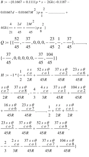
Coefficient Matrices T, Q and F and Constant matrices B, H, A.

2 2

52 37

: {{ ,

45 30 30 15 45 30 30 2

7 23 2 2 7 1

, 0, 0, 0, ,

90 45 45 45 90 2 90

2 2

2 37

, }

90 45 45 30 30 9

d M s d M

F

s d M s d

M s d M s

      

     

    

2 2

37 2

, ...{ , ,

45 30 30 9 9 9 9

2 2

2 37 0, 0, 0,

9 9 9 45 30 30

2 104 8 8

, }}

9 45 45 45

d M s d M s

d M s d M

s d M

      

      

 

1 1 1

: 1* ( ( 1 ) ( )

1 1

30 60 30

1 2 1

( ) ( ) ( )

2 2 6 6 7 7

30 45 90

1 1 1

( ), ..., ( ) ( )

8 8 1 1 2 2

30 30 9

1 1 8

( ) ( ) ( )}

6 6 7 7 8 8

9 30 45

R

A R R c

R c R c R c



  



       

     

       

     

: {{1.156 0.06667 * , 0.8222

0.07778 * , 0, 0, 0, 0.5111 0.07778 * , 0.5

0.04444 * , 0.8222 0.1111 * }, ...,

2 *

{ 0.8222 0.1111 * , , 0, 0, 0, 9

2 * 104

, 0.8222 0.1111 * , }}

9 45

T p s

p s p s

p s

   

 

  

  

 

: {0.1667 0.1111 * 2 ( 0.1187

2 2

0.01667 0.01667 ) ... 1

2

4 2 2 2

4 ( ) }

8 21 45 45

B p s Gk

d M p u

d M

Gk p u

     

  

 

52 37 23 1 37

: {{ , , 0, 0, 0, , , }, ...,

45 45 45 2 45

37 37 104

{ , 0, 0, 0, 0, 0, , }}

45 45 45

Q    

 

1

52 37 23

1 ₁ ₂ ₆

: 1 * {

2 2 45 45 45

37 ₄ 4 37 104

7 8_, 1 2

2 45 3 3 45 45

16 23 ₁

6 7

, ...,

45 45 2 2 2

23 37 52

2 6 7

45 45 45

s s s s s s s s

c o c o c o c o

H

R R R R

s s s s s s s s s s

c o c o c o c o c o

R R R R R

s s s s s s s s

c o c o c o c o

R R R R

s s s s s s

c o c o c o

R R R

  

   

  

      

    

   

  

 37

8 , 45

2 37 37 104

2 ₁ ₇ ₈

}

3 3 45 45 45

s s c o

R

s s s s s s s s

c o c o c o c o

R R R R



  

    

Next we should find Coefficient matrix for temperature equation by executing the below command

[

[ , ],{ ,1,8},{ ,1,8}]

i j

Table Coefficient t



i

j

Next we should find constant matrix for temperature equation by executing below two commands

[

0,{ ,1,8}];

i

Do





i

[ ,{ ,1,8}]

i

Table t i

By Serendipity element the velocity, temperature and concentration equations are given below

1

*

1 2

*

2 6

*

6 7

*

7 8

* ;

8

w



u n u n u n u n u n



1

*

1 2

*

2 6

*

6 7

*

7 8

*

8 3 4 5

;

t





n





n





n





n





n n n n

  

1

*

1 2

*

2 6

*

6 7

*

7 8

*

8 3 4 5

;

(6)

1

: 2( 1 ) 4( )( 1 )

4 2

1

2 4( 1 ) 2( )

2 1

4( )( 1 ) +4(-1+y) c 4 c

1 2 6

4 2

1 1

4( ( 1 ) c 4( 1 ) c

7 8

4 2

y

wed y y

y y y y y

y

y c y

y y y y

        

      

     

      

Iterations for finding Sherwood number values

[

5;

2000;

0.8;

0.5;

1.3;

0.5;

2000;

1;

0;

0.71;

1;

c o

Do M

G

s

k

s

d

R

y

p

z



1 2 3 4 5 6 7 8

{ , , , , , , , } {0, 0, 0, 0, 0, 0, 0, 0};

u u u u u u u u



1 2 3 4 5 6 7 8

{ , , , , , , , }

       



Inverse T B

[ ]. ;

{ , , , , , , , }

c c c c c c c c

1 2 3 4 5 6 7 8



Inverse Q H

[ ]. ;

1 2 3 4 5 6 7 8

{ , , , , , , , }

u u u u u u u u



Inverse F A

[ ]. ;

{ , , , , , , , }

       

1 2 3 4 5 6 7 8



Inverse T B

[ ]. ;

1 2 3 4 5 6 7 8

{ , , , , , , , }

c c c c c c c c



Inverse Q H

[ ]. ;

{ , , , , , , , }

u u u u u u u u

1 2 3 4 5 6 7 8



Inverse F A

[ ]. ;

1 2 3 4 5 6 7 8

{ , , , , , , , }

       



Inverse T B

[ ]. ;

&&TableForm[Table[wed]]

Output -1.31629

We should calculate Sherwood number Values at y=0 and y=1 levels. At every iteration changing one parameter and remaining other parameter values fixed we get all parameter values at y=0 and 1 levels

.

V.DISCUSSION OF THE NUMERICAL RESULTS

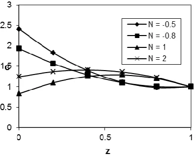
The main aim of this problem is to investigate the rate of mass transfer on the free and forced convective heat and mass transfer flow of a viscous, incompressible fluid through a porous medium contained in a porous vertical channel. The Concentration profiles are drawn at different vertical levels normal to the walls in figs (1) – (4). The Concentration distribution (C) with N at y=0, y=1, z=0, z=0.5 is shown in figs.1-4.

When the molecular buoyancy force dominates over the thermal buoyancy force the concentration

depreciates when the buoyancy forces act in the same direction and for the forces acting in opposite directions C experiences an enhancement at all levels. (figs 1-4).

Fig. 1 Variation of C with N at y = 0 level.

D-1 =2x103,G=2x103, Ec = 0.5 ,So = 0.5 ,S = 0.8, Sc= 1.3

Fig. 2 Variation of C with N at y = 1 level. D-1 =2x103 , G=2x103, Ec = 0.5 , So = 0.5 , S = 0.8 , Sc = 1.3

(7)

Sc = 1.3

Fig. 4 Variation of C with N at Z = 0.5 level.

D-1 =2x103 , G=2x103, Ec = 0.5 , So = 0.5 , S = 0.8 , Sc = 1.3

Table – 1

Sherwood Number (Sh) at y = 0 Level Sc = 1.3, So = 0.5, N = 1, P = 0.71,

Ec = 0.5, P = 0.71

G I II III

2 x 103 -1.31629 -0.594953 -0.353811 5 x 103 -3.12223 -1.3189 -0.716047 8 x 103 -4.92818 -2.04285 -1.07828

104 -6.13215 -2.52549 -1.31977

IV V VI

-0.716626 -0.681856 -0.508086

-1.42926 -1.39771 -1.24018

-2.14189 -2.11356 -1.97228

-2.61697 -2.5908 -2.46035

I II III

D-1 2 x 103 5 x 103 104

S 0.8 0.8 0.8

IV V VI

5 x 103 5 x 103 5 x 103

0.1 0.3 1.3

Table – 2

Sherwood Number (Sh) at y = 1 Level Sc = 1.3, So = 0.5, N = 1, P = 0.71, Ec = 0.5, P = 0.71

G I II III

2 x 103 0.459581 1.20745 1.4574

5 x 103 -1.41257 0.4571 1.08198

8 x 103 -3.28472 -0.293248 0.706555

104 -4.53282 -0.79348 0.456273

IV V VI

1.08593 1.12066 1.2942

0.347136 0.378571 0.535542

-0.391659 -0.363514 -0.22312

-0.884189 -0.858238 -0.728895

I II III

D-1 2 x 103 5 x 103 104

S 0.8 0.8 0.8

IV V VI

5 x 103 5 x 103 5 x 103

0.1 0.3 1.3

The Sherwood number (Sh) which measures the rate of mass transfer at y=0 level and y=1 level is exhibited in tables 1&2 for variation in G, D-1, Sc, S, So, Ec and N. It is found that the rate of mass

transfer is negative for all variations at y=0 level. An

increase in G enhances

Sh

at both levels. The variation of Sh with D-1 shows that lesser the

permeability of the porous medium depreciates

Sh

at y = 0 level and enhances it at y = 1 level. Also an increment in the suction parameter S leads to a

reduction in

Sh

at y = 0 level and enhancement in

Sh

for level G≤5x103 but for higher G≥8x103,

Sh

depreciates with S (tables 1 & 2).

VI. CONCLUSIONS

1. By using Mathematica 4.1 commands we

executed and calculated Sherwood number values for different parameters.

2. It is found that the rate of mass transfer is negative for all variations at y=0 level .

3. It is found that an increase in G enhances

Sh

at both levels.

REFERENCES

[1]. A. Barletta and D. A. Nield , “Combined Forced and Free Convective Flow in a Vertical Porous Channel: The Effects of Viscous Dissipation and Pressure Work”, Trans Porous Medium., vol.79, pp. 319–334, 2009.