Observer-Based Hierarchical Sliding Mode Control of
Uncertain Underactuated Systems with Time Delay and
Input Saturation
Chiang-Cheng Chiang*, Pen-Chun Lu
Department of Electrical Engineering, Tatung University, Taipei, Taiwan, Republic of China
Abstract This paper considers the problem of observer-based hierarchical sliding mode control approach for uncertain
underactuated systems with time delay and input saturation in strict-feedback form. Based on sliding mode control technique and the concept of hierarchical design, an adaptive fuzzy hierarchical sliding mode controller is designed for the uncertain nonlinear system by using fuzzy logic systems to approximate the uncertain functions. Additionally, input saturation which is one of the most important input constraints usually appear in many industrial control systems. By choosing an appropriate Lyapunov–Krasovskii function, the proposed controller is designed to demonstrate that all the signals in the closed-loop system can not only guarantee uniformly ultimately bounded, but also achieve good tracking performance. Finally, some computer simulation results of a practical example are illustrated to verify the effectiveness of the proposed approach.Keywords
Underactuated system, Lyapunov–Krasovskii function, Strict-feedback form, Hierarchical sliding mode control, Time delay, Input saturation, Fuzzy logic systems1. Introduction
During the past decades, underactuated systems have drawn much attention and some significant results have been obtained in the literature. Wu et al. [1] cope with the problem of fault detection for underactuated manipulators. Lai et al. [2] deal with the problem of the stable control strategy for the planar three-link underactuated mechanical system. Recently, for systems with special structure, i.e. strict-feedback form, many research results have been proposed in [3-5]. In this paper, the underactuated systems in strict-feedback form are investigated and some systematic methodologies are proposed to solve the tracking control problem.
In practice, input saturation is one of the most important input constraints which are usually utilized in many industrial control systems. In addition, because saturation is a potential factor degrading the control system performance, it often gives rise to undesirable inaccuracy, or even affects system stability. In recent years, Chen et al. [6] introduced an adaptive neural-network backstepping control approach for a class of uncertain nonlinear systems in the presence of
* Corresponding author:
[email protected] (Chiang-Cheng Chiang) Published online at http://journal.sapub.org/ajis
Copyright©2019The Author(s).PublishedbyScientific&AcademicPublishing This work is licensed under the Creative Commons Attribution International License (CC BY). http://creativecommons.org/licenses/by/4.0/
input saturation. Liu et al. [7] investigated the problem of the observer-based neural control method for MIMO pure-feedback non-linear systems with input saturation and disturbances.
A general sliding-mode control (SMC) is established in this paper for a class of uncertain underactuated systems. As a kind of highly robust variable structural control method, the sliding-mode controller is able to respond quickly, insensitivity to systemic parameters, good transient performance, external disturbance, and so on. Due to the underactuated characteristic of the controlled system, at least two sliding surfaces with specific relation are employed for the controller design. For the aggregated hierarchical structure of a sliding-mode controller, the underactuated system is segmented into several subsystems. For each part, we design a first-layer sliding surface. Then, the first-layer sliding surfaces are utilized to construct the second-layer sliding surface. By theoretical analysis, the conclusion is made that all sliding surfaces of the SMC structure is asymptotically stable.
The main contribution of this paper is that the proposed hierarchical sliding mode control method deals with the problem of tracking performance and stability for a class of underactuated systems in strict-feedback form with input saturation and time delay. Based on sliding mode control technique and the concept of hierarchical design, an adaptive fuzzy hierarchical sliding mode controller is designed for the underactuated system by using fuzzy logic systems to approximate uncertain functions. The fuzzy state observer is employed to estimate the unavailable state for measurement. Choosing an appropriate Lyapunov-Krasovskii function, it is theoretically ensured that all the signals in the closed-loop system are uniformly ultimately bounded and obtain good tracking performance under our designed controller.
The remainder of the paper is organized as follows. Section II describes the problem formulation and preliminaries together with the definition of fuzzy logic systems (FLSs) are given. In Section III, adaptive fuzzy hierarchical sliding mode controller and observer are designed for a class of uncertain underactuated nonlinear time-delay systems with saturation input and the stability analysis of the whole system is also verified by Lyapunov-Krasovskii functional. Some computer simulation results of a practical example are demonstrated to show the effectiveness of the proposed approach in Section IV. Finally, the conclusion is drawn in Section V.
2. Problem Statement and Preliminaries
2.1. Problem StatementConsider a class of single-input-multi-output uncertain underactuated nonlinear systems in strict-feedback form with input saturation expressed as follows:
11 12
( ( )) ( ( )) ( , )
12 1 1 1
21 22
( ( )) ( ( )) ( , )
22 2 2 2
1 2
( ( )) ( ( )) ( , )
2
( ) [11 21, ,..., 1]
x x
x f t sat u t d t
x x
x f t sat u t d t
xn xn
xn fn n t sat u t dn t
T
t x x xn
τ τ τ = = − + + = = − + + = = − + + = x x x x x x y (1)
Eq. (1) can be rewritten as
[
sat( ( ))u t ( t τ ) ( , )t]
= + + +
=
x Ax B f x( - ) D x
y Cx
(2)
where
2 2
0 1 0 0 0 0
0 0 0 0 0 0
0 0 0 1 0 0
,
0 0 0 0 0 0
0 0 0 0 0 1
0 0 0 0 0 0
n n×
= ∈ℜ A 2
0 0 0 0 0 0
1 0 0 0 0 0
0 0 0 0 0 0
= 0 1 0 0 0 0 ,
0 0 0 0 0 0
0 0 0 0 0 1
n n×
∈ℜ B 2
1 0 0 0 0 0
0 0 1 0 0 0
0 0 0 0 0 0
= 0 0 0 0 0 0 ,
0 0 0 0 0 0
0 0 0 0 1 0
n n×
∈ℜ C 1 1 2 2 3 3 1 4 4 1 1 1 2 3 1 4 1 ( ( )) ( ( )) ( ( )) ( ( )) ( ) , ( ( )) ( ( )) ( , ) ( , ) ( , ) ( , ) , , ( , ) ( , ) n n n n n n n n f t f t f t f t t f t f t d t d t d t d t t d t d t τ τ τ τ τ τ τ × − − × − − − − − − = ∈ℜ − − = ∈ℜ x x x x f(x ) x x x x x x D(x ) x x 1 ( ) ( ) ) ( )
sat ( ) ( ) ,
( ) ( )
n
sat u t sat u t
sat u t u t sat u t
sat u t sat u t
where x =
[
x x11 12, ,...,x xn1, n2]
T is the system state vector which is assumed to be unavailable for measurement,(t)
u ∈ℜand y∈ℜn are input and output of the system, respectively. τ is the value of time delay.
1 1( ( )), ( (2 2 )), , ( (n n ))
f x t−τ f x t−τ f x t−τ are unknown real continuous nonlinear functions where T
1 2
[ , ] i = x xi i
x , for
𝑖𝑖 = 1,2, … , 𝑛𝑛 , and d1( , ), ( , ), ,xt d2 xt dn( , )xt are unknown external bound disturbances. sat u t( ( )) denotes the nonlinear saturation characteristic. Without loss of generality, the following assumptions are made for the controller design:
Assumption 1: The time delay is a fixed and known constant.
Assumption 2: 0 < ( )fi x ≤Fi < ∞, i=1,2, ,n for all x, where Fi are known positive constants.
In order to deal with the control constraints for convenience, the saturation function 𝑠𝑠𝑠𝑠𝑠𝑠(𝑢𝑢(𝑠𝑠)) can be rewritten as
𝑠𝑠𝑠𝑠𝑠𝑠(𝑢𝑢(𝑠𝑠)) = 𝜒𝜒(𝑢𝑢(𝑠𝑠)) ∙ 𝑢𝑢(𝑠𝑠) (3) where 𝜒𝜒(𝑢𝑢(𝑠𝑠)) be expressed as
𝜒𝜒(𝑢𝑢(𝑠𝑠)) = � 𝑢𝑢𝑚𝑚/𝑢𝑢 , if 𝑢𝑢 > 𝑢𝑢1 , if −𝑢𝑢𝑚𝑚 ≤ 𝑢𝑢 ≤ 𝑢𝑢𝑚𝑚 𝑚𝑚
−𝑢𝑢𝑚𝑚/𝑢𝑢, if −𝑢𝑢𝑚𝑚 > 𝑢𝑢
(4)
Assumption 3: 0 < ‖𝐃𝐃(𝐱𝐱, t)‖ ≤ ℎ < ∞, where is an unknown constant.
Control Objective: Design a controller for (1) such that the system output ( )yt would track the desired output vector yd( )t , where yd( )t is the bounded desired signal
and contains the finite derivative up to the second order. Define the vector of the output tracking error as
( )t ( ) [ , ,..., ]t e e1 2 e T n
d n
= − = ∈ℜ
e y y (5)
2.2. Description of Fuzzy Logic Systems
The fuzzy logic system performs a mapping from n
U ⊂ ℜ toV ⊂ ℜ. Let U U= 1× × Un whereUi⊂ ℜ,
1,2, ,
i= n. The fuzzy rule base consists of a collection of fuzzy IF-THEN rules:
( )
1 1 2 2
: IF is , and is , and and, is THEN is , for 1,2, , .
l l l l
n n l
R x F x F x F
y G l= M
(6)
in which x=
[
x x1 2, , , xn]
T∈U and y V∈ ⊂ ℜ are the input and output of the fuzzy logic system, Fil and Gl are fuzzy sets in Ui and V , respectively. The fuzzifier maps a crisp point x=[
x x1 2, , , xn]
T into a fuzzy set in U . The fuzzy inference engine performs a mapping from fuzzysets in U to fuzzy sets in V , based upon the fuzzy IF-THEN rules in the fuzzy rule base and the compositional rule of inference. The defuzzifier maps a fuzzy set in V to a crisp point in V . The fuzzy systems with center-average defuzzifier, product inference and singleton fuzzifier are of the following form:
( ) T
y=θ ξ x (7)
where θT = θ1, ,θM with each variable θl as the point at which the fuzzy membership function of Gl achieves the maximum value and ξ x( )= ξ1( ),...,x ξM( )xT with each variable ξl( )x as the fuzzy basis function defined as
1
1 1
( ) ( )
( )
n l i
i F
l i
M n
l i i Fi l
x
x
µ ξ
µ
= = =
=
∏
∑ ∏
x (8)
where µFil( )xi is the membership function of the fuzzy set.
3. Controller Design and Stability
Analysis
First, let the unknown nonlinear functions (f x( - )t τ ) can be approximated, over a compact set Γ, by the fuzzy logic systems as follows:
ˆ( (t−τ) |ˆf)=ˆTf f( (t−τ))
f x θ θ ξ x (9)
where ξf( (xt−τ)) is the fuzzy basis vector, ˆθTf is the
corresponding adjustable parameter vectors of each fuzzy logic systems.
Owing to the unavailable states of the system in many practical systems, the fuzzy logic system (9) is not used to control nonlinear systems whose states are not obtained for measurement. Therefore, an observer is employed to estimate the unavailable states. Now, let ˆx be defined as the estimates of x. Then, we can obtain the following fuzzy logic systems as
ˆ( (ˆ t−τ) |ˆf )=ˆTf fξ ( (ˆ t−τ))
f x θ θ x (10)
In order to estimate the state, we design the observer for system (2) as follows:
ˆ ˆ
ˆ ˆ sat( ( )) ˆ ˆ
ˆ ˆ
u t t τ f
−
x = Ax+B +f(x( )| )+v +L(y-y) y = Cx
θ
(11)
1 1
2 3 2
2 1
4
1
0 0 0 0 0
0 0 0 0 0 0
0 0 0 0 0
, ,
0 0 0 0 0 0
0 0 0 0 0
0 0 0 0 0 0
n n n
n n
n v l
v v l
v
R R
v l
v
× ×
−
= ∈ = ∈
L v
L is the observer gain matrix to guarantee the characteristic polynomial of A LC− to be Hurwitz. Let us define the estimation error vector as x x x= −ˆ and
ˆ = −
y y y , then by (2) and (10), we obtain
(
)
ˆ ˆ ˆ ,t
t τ t τ f
− −
x = A-LC x+B f(x( ))-f(x( )| )+D(x )-v y = Cx
θ
(12)
It is assumed that x, ˆx, and ˆθf belong to compact sets Ωx, Ωxˆ, ˆ
f
Ωθ , respectively, which are defined as
{
}
:Rn N
Ω =x x∈ x ≤ x< ∞ (13)
{
}
ˆ :ˆ Rn ˆ Nˆ
Ω =x x∈ x ≤ x< ∞ (14)
{
}
ˆf ˆf RM : ˆf Nf
Ωθ = θ ∈ θ ≤ < ∞ (15)
where Nx, Nˆx, and Nf are the designed parameters, and M is the number of fuzzy inference rules. Let us define the optimal parameter vector θ∗f as follows:
* arg min sup ( ) ˆ ˆ( )
f f
f∈Ω f ∈Γ
= −
θ θ x
θ f x f xθ (16)
where θ*f is bounded in the suitable closed set Ωθf . The parameter estimation errors can be defined as
*
f f f
θ = θ - θ (17) and
ˆ
( (t τ)) ( (t τ) | ∗f)
= − − −
w f x f x θ (18)
is the minimum approximation errors, which correspond to approximation errors obtained when optimal parameters are used.
Applying (17) and (18) into (12), we obtain
(
)
( (ˆ )) + ( ,t).
T
f f t τ
= − + − + −
=
x A LC x B x w D x v
y Cx
θ ξ
(19)
The output error dynamics of (19) can be expressed as follows:
ˆ
( )[s Tf f( (t τ)) + ( ,t) ]
= − + −
y H θ ξ x w D x v (20)
where
(
)
(
)
1( )s = s − − −
H C I A LC B (21) and s denotes the complex Laplace transform variable. As has been discussed, we could not obtain all elements of x, because not all states of the system are available for measurement. Hence, we could not obtain all elements of x. We will employ the state variable filters [11] to cope with this problem. First, we choose a stable filter G su( ) as the following form:
0 0
1
( ) , for 0 u
G s g
s g
= >
+ (22)
And
[
]
( )s =diag G s G su( ), u( ), ,G su( ) ∈ n n×
G R (23)
Introducing (23) into (20), we can obtain the steady-state equation
{ }
1 ˆ
( ) ( )s s − = ( )s Tf f( (t−τ))+ + ( ,t)−
G H y G θ ξ x w D x v (24)
Define a set of state variable filters Ti( )s =G( ) ,s si
0,1
i
=
, thus,0 0
0 1
1 0
0 1 ( ) ( )
( ) ( ) ( )
s s s
s g s
s s s T s s
s g
= =
+
= = =
+
T G
T G
(25)
The corresponding filtered signals are defined as follows:
{ }
{ }
0 1 1
1 1 2
, for 1, 2, ,
fi i
fi i
T
i n
T
=
=
=
x x
x x
(26)
{ }
0( )
f = s
w T w (27)
{ }
0( )
f = s
ξ T ξ (28)
{ }
0( )
f = s
v T v (29) and
{
}
0
( ) ( ) ( , ) f t =T s t
D D x (30) Then, Eq. (19) can be rewritten as follows:
(
)
( (ˆ )) + ( ,t)
T f
f f f f f f
f
t τ
= − + − + −
=
x A LC x B x w D x v
y Cx
θ ξ
(31)
where [ , ,..., , ] 2 ,
11 12 n1 2T n
x x x x
f = f f f fn ∈ℜ
x
We define
ˆ
h = h h − (32) and
1 1− ˆ1
where ˆw1 and ˆh are the estimated of w1 and h , respectively.
where
1
w ≥ wf (34) Based on Lyapunov stable theorem, we can obtain the robust compensation term vf and the parameter update
laws as follows:
ˆ
ˆ1 h
T T
f f
f T T
f f
=B Px +B Px v
x PB x PB
w (35)
ˆf =γf f ˆ t - τ Tf
θ ξ (x( ))x PB (36)
ˆw1 w1 =γ x PBTf (37)
ˆh T
h f γ
= x PB
(38) where
γ
f, γh, γw1 are positive constants.Remark 1: Without loss of generality, the adaptive laws used in this paper are assumed that the parameter vectors are within the constraint sets or on the boundaries of the constraint sets but moving toward the inside of the constraint sets. If the parameter vectors are on the boundaries of the constraint sets but moving toward the outside of the constraint sets, we have to use the projection algorithm to modify the adaptive laws such that the parameter vectors will remain inside of the constraint sets. Readers can refer to reference [10]. The proposed adaptive law (35)-(38) can be modified as the following form:
{
}
ˆ
ˆ t τ , if ( ) or (
T ˆ
and t τ 0) ˆ t τ , if (
f
T f N
f f f f
N
f f
T f
f f
T
P f f f f Nf
γ γ = − < = ⋅ − ≥ − = θ
(x( ))x PB
x PB (x( ))
(x( ))x P B ξ θ θ θ ξ ξ θ
T ˆ
and Tf f f t τ 0)
⋅ − <
x PB θ ξ (x( ))
(39)
where P
{
γf fx P (x(T ξf ˆ t - τ))}
is defined as{
}
T 2 ˆ t τ
ˆ ˆ
ˆ t τ ˆ t τ
ˆ
T
f f f
f f
T T
f f f f f f
f
P γ
γ γ
−
= − + −
x PB (x( ))
θ θ
(x( ))x PB x PB (x( ))
θ
ξ
ξ ξ (40)
The main result of robust adaptive fuzzy observer scheme is summarized on the following theorem.
Theorem 1: Consider the single-input-multi-output
uncertain underactuated system (1). The robust adaptive fuzzy observer is defined by (10) with adaptation laws given by (35)-(38). For the given positive definite matrix Q, if there exist symmetric positive definite matrix P such that the following Lyapunov equation
(
A LC P P A LC = Q−)
T +(
−)
− (41)is satisfied, then all the closed-loop signals are bound, and the estimation errors converge to a neighborhood of zero.
Proof. Consider the Lyapunov function candidate
( ) ( )
T 21 1
h 1
1 1 1 1 w 1 h
2 Tf f f Tf f f f f w
V tr tr
γ γ γ γ
= + + +
x Px θ θ θ θ
(42)
2 3
1 2
V = S (43)
2 1 ˆ ˆ ( ) θˆ 4 2 1
t n
V f x zi i fi dz
i t τ
= ∑ ∫
= −
(44)
By the time derivative of V1 and the facts θf = −θˆ ;f
1 1
ˆ ˆ
h = −h ; w = −w we obtain
(
)
(
)
{
}
(
( )
)
( )
T T
1
T T T T
1 1 h 1
1 + ˆ
2
1 ˆ
+
1 ˆ 1 ˆ
w w hh
T T
f f f f f
f f f f f f f f
f w V t tr τ γ γ γ = + + − − − −
x A LC P P A LC x x PBθ ξ x
-x PBw x PBD x PBv θ θ
(
)
(
)
{
}
(
( )
)
( )
TT T T
T T T T
1 1 h 1 1 ˆ + 2 1 ˆ + +
1 ˆ 1 ˆ
w w hh
f f f f f
f f f f f f f f
f w t tr τ γ γ γ ≤ − + − − − − −
x A LC P A LC x x PBθ ξ x
-x PB w x PB D x PBv θ θ
(45) Applying Assumption 3 and (34) yields
(
)
(
)
{
}
(
( )
)
( )
(
)
(
)
{
}
( )
(
)
T T 1T T T T
1 1 1
1
h
T
T T T
1
T T T T
1 + ˆ
2
1 ˆ 1 ˆ
+ w h w w
1 ˆ hh
1 + wˆ hˆ
2 1 ˆ ˆ + T T
f f f f f
f f f f f f
f w
f f f f
f f f f f f
f
V t
-tr t tr τ γ γ γ τ γ ≤ + + − − − − = − + − + − −
x A - LC P P A - LC x x PBθ ξ x
x PB x PB x PBv θ θ
x A LC P A LC x x PB x PB
x PBv x PBθ ξ x - θ
( )
f
θ
T T
1 1
h 1
1 ˆ 1 ˆ
+w f w +h f h
w γ γ − −
x PB x PB
(46)
By employing (35)-(38), we can get
(
)
(
)
{
}
T1 1
T T
1 + wˆ
2 ˆ h
T T
f f f
f f f
V ≤ +
+ −
x A - LC P P A - LC x x PB
x PB x PBv
(47)
Then using the robust compensation term vf as shown
in (35), the above equation can be rewritten as
(
)
(
)
{
}
1 12 Tf T f
V ≤ x A - LC P P A - LC x+ (48) According to (41), it can be easily shown that
1 12 Tf f
V ≤ − x Qx (49) Therefore, it can be concluded that V1≤0 from (49), and the estimation errors of the closed-loop system converges asymptotically to a neighborhood of zero based on Lyapunov synthesis approach. This completes the proof.
Next, we design the observer-based incremental sliding mode controller. Define the sliding surfaces as follows:
i i i i
s =c e +e , for i=1, 2,…, n, (50) where ci are positive constants.
Differentiating si with respect to time and from (5), we have
2
ˆ
( ) [ ]
i i i i
i ii di i i i
s c e e
c e y t x l y
= + = + − + ˆ ˆ ˆ ( ) ( ( ) | )
( ( )) v }
i i di i i fi
i i i
c e y t f t
sat u t l y
τ = + − − − − − x θ (51)
Then, the second-level sliding surface can be defined as follows:
1 1 2 2 ... n n
S=α s +α s + +α s (52) where αi , for i=1,2,…,n, are sliding mode parameters which maybe remain constant or change according to different conditions.
Based on the fuzzy logic systems and the states of the system are not obtained for measurement, the equivalent control law can be obtained as
(
)
(
)
( )
( )
( )
1
2 2
2 2 2
( )
5 1 1 1 1
2 2 2 i 2 2
eqi i
i i i d i i i
u S
S c e y v l y
α δ α − = + + + + (53)
and vi can be obtained by backward from vf .
Then we define:
1
n
eqi sw i
u u u
=
=
∑
+ (54)where
(
)
1
1
2
1 1 1
( )
1 ˆ ˆ ˆ
( ) ( )
2 n
sw i
i
n n n
i eqr i i fi
i r i
r i u
u f x t KS
S δ α δ α − = = = = ≠ = − − −
∑
∑
∑
∑
θ (55)for a positive constant K.
Theorem 2: Consider the single-input-multi-output underactuated system (1). If Assumptions 1-3 are satisfied, then the proposed adaptive fuzzy sliding mode controller defined by (54) with adaptive laws (35)-(38) guarantees that all signals of the closed-loop system are bounded, and the output tracking errors converge to a neighborhood of zero. If the choice of αi, which ensures that ( ) 0
1
n i i
δ ∑ α ≠
= , satisfies
0 , if 0 , if 0 0 s i i i s i i α α α ≥ = − ≥
(α0i >0, for =1,2,..., -1i n ) (56)
and αn =1 such that αi is , for i=1,2,…,n-1 and sn are the same sign. Then, the first-level sliding surfaces
1 2, ,..., n
s s s are also asymptotically stable. Proof:
Consider the Lyapunov function candidate V2=V3+V4. Differentiating the V3 and V4 with respect to time, we can obtain ( ( ) 3 1 ˆ ˆ ˆ ( ( ) θ ) 1 n
V S i i ic e yd sat u t v l yi i i i
i n
S i fi i t fi i α α τ = ∑ + − − − = + ∑ − − = x (57) 2 2
1 ˆ ˆ ( ) θˆ 1 ˆ ˆ ( ) θˆ
4 2 1 2 1
n n
V fi i t f fi it f
i i
i i τ
= ∑ − ∑ − = x = x
(58)
With the use of 2ab a≤ 2+b2for scalars a and b, we obtain
( )
( )
( )
[ ]
( )
( )
( )
( )
( )
2
2 2 2
1 1 1 1
3 2 2 2 2
1 1 1 1
2 2
1 1
+ ( ( ) +
2 2
1 1 1
2 2 2
1 + 1 + 1
2 2 2
1 1 1
2 1 ˆ ˆ ˆ
+ ( ) θ
2
n n n n
V S i c ei i S i ydi
i i i i
n n n
S i sat u t S i vi
i i i
n n n
S i l yi i S i
i i i
fi i t fi
α α α α α α τ ≤ ∑ + ∑ + ∑ + ∑ = = = = − + ∑ ∑ ∑ = = = + ∑ ∑ ∑ = = = − x
1
n i∑=
( )
( )
( )
[ ]
( )
( )
( )
( )
( )
2
2 2 2
1 1 1 1
2 2 2 2 2
1 1 1 1
2 2
1 1
( ( ) +
2 2
1 1 1
2 2 2
1 1 1
2 2 2
1 1 1
2 1 ˆ ˆ ˆ + ( ) θ
2
n n n n
V S i c ei i S i ydi
i i i i
n n n
S i sat u t S i vi
i i i
n n n
S i l yi i S i
i i i
fi it fi
α α
α α
α α
≤ ∑ + ∑ + ∑ + ∑
= = = =
+ ∑ − ∑ + ∑
= = =
+ ∑ + ∑ + ∑
= = =
x
1
n i
∑
=
(60)
By introducing (3) into (60), we obtain
( )
( )
[
]
( )
( )
2
2 1 2 1
3
2 2 2
1 1 1
2 2
1 1
( ) ( )
2 2
1 1 1
2 1 ˆ ˆ ˆ
2 ( ) θ 1
n n n
V S i c ei i ydi
i i i
n n n
S i u u t vi l yi i
i i i
n
fi it fi i
α
α χ
≤ ∑ + ∑ + ∑
= = =
− ∑ + ∑ + ∑
= = =
+ ∑
=
x
(61)
since 0<χ( ( )) 1u t ≤ according to the density property of a
real number [12], there exists a constant δ that satisfies
(
)
0< ≤δ min ( ( )) 1χ u t ≤ (62)
( )
2 1( )
2 1 2 1( )
2 1( )
2 32 2 2 2 2
1
2
1 ˆ ˆ ˆ
( ) θ
2
1 1
n
V S i c ei i yd vi l yi i i
i
n n
S i ueqr usw fi i t fi
r i
α
α δ
≤ ∑ + + + +
=
− ⋅ ∑ + + ∑
= =
x
(63)
Then substituting the equivalent control ueqi in (53) into (63), we have
2 1 ˆ ˆ ( ) θˆ
2 2
1 1 1
n n n
V S i ueqr usw fi it fi
i r i
r i
δ α
≤ − ∑ ∑ + + ∑
= = =
≠
x
(64)
Using the switching control law (53), one can obtain
2
2 0
V ≤ −KS ≤ (65)
Therefore, it can be concluded that V2 ≤0 from (65), and all the signals of the closed-loop system converge asymptotically to a neighborhood of zero based on the Lyapunov synthesis approach. This completes the proof.
4. An Example and Simulation Results
In this section, a mass-spring-damper system [8] in the presence of uncertain parameter and exogenous disturbances is considered as our simulation example as shown in Fig. 1, and described by the following form:
11 12
( ( )) ( ( )) ( , )
12 1 1 1
21 22
( ( )) ( ( )) ( , )
22 2 2 2
x x
x f t sat u t d t x x
x f t sat u t d t
τ
τ =
= − + +
=
= − + +
x x
x x
(66)
[
11 21]
( )t = x x, T
y where
{
}
1
( ( )) { }
1 1 1 1
1
3 2
211( ) 0.511( ) 212( ) 0.6512( ) 1
f t fK fB
M
x t x t x t x t
M
τ
τ τ τ τ
− = − −
− − − − − − − − =
x
{
}
1
( ( )) { }
2 2 2 2
2
3 2
2 21( ) 0.5 21( ) 2 22( ) 0.5 22( ) 2
f t fK fB
M
x t x t x t x t
M
τ
τ τ τ τ
− = − −
− − − − − − − − =
x
and x x11, 21 are the displacement of the mass, x x12, 22 are the velocity of the mass, fK1 and fK2 are the spring force,
1
B
f and fB2 are the friction force. M1 =10Kg, 11Kg M2 = are
the body mass, and sat u t( ( )) is the force of saturation. The disturbances are assumed to be d1( , ) 0.1 ( )cos( )xt = x t12 t and
2( , ) 0.122( )cos( )
d xt = x t t .
1
K
f
1
B
f
2
K
f
Actuator (u)
Actuator (u)
u(t) 2
B
f
2 K2 K
sat(u(t))
sat(u(t))
1 M
2 M
In the implementation, six fuzzy sets are defined over interval [-3, 3] for x x x1, , and 2 3 x4, with labels NB, NM, NS, PS, PM, and PB, and their membership functions are
( )
(
1(
)
)
1 exp 5 2
NB i
i
x
x
µ =
+ − + ,
( )
(
)
(
2)
1 1 exp 1.5
NM i
i
x
x
µ =
+ − + ,
( )
(
)
(
2)
1
1 exp 0.5
NS i
i x
x
µ =
+ − + ,
( )
(
)
(
2)
1 1 exp 0.5
PS i
i
x
x
µ =
+ − − ,
( )
(
)
(
2)
1 1 exp 1.5
PM i
i
x
x
µ =
+ − − ,
( )
(
1(
)
)
1 exp 5 2
PB i
i
x
x
µ =
+ − − ,i=1,2,3,4.
Figure 2. The outputs 𝑥𝑥11 and 𝑦𝑦𝑑𝑑1
Figure 3. The outputs 𝑥𝑥21 and 𝑦𝑦𝑑𝑑2
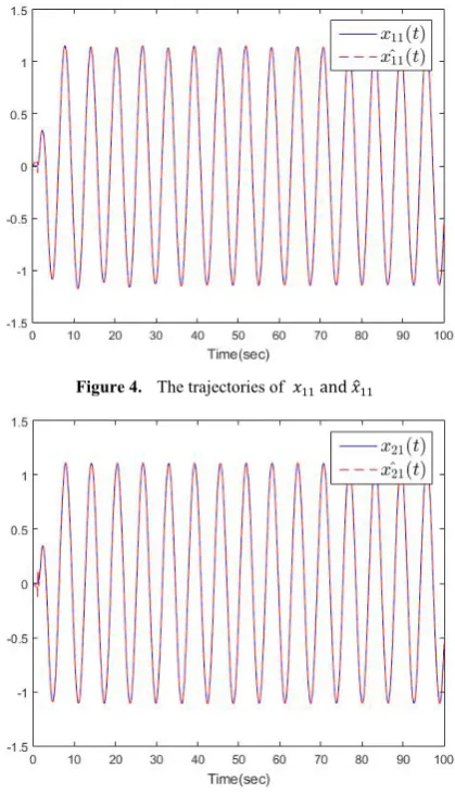
Figure 4. The trajectories of 𝑥𝑥11 and 𝑥𝑥�11
Figure 5. The trajectories of 𝑥𝑥21 and 𝑥𝑥�21
In this case, the control objective is to maintain the system output y to follow the reference signal yd1=1.1sin( )t and yd2=1.1sin( )t . First, we select the observer gain matrix as 10 0 0 0
0 0 10 0
T
L = . The sliding surfaces are selected as s1=c e e1 1+1 and s2=c e2 2+e2 , where
1 2 0.9
c =c = , the second-level sliding surface is constructed as S=α1 1s +α2 2s , where α01=1.1 and α02=2. The initial values are chosen asxˆ(0) [0,0,0,0]= T,x(0) [0,0,0,0] ,= T
1(0) 0.55
f
θ = − , θf2(0)= −0.55, ˆh(0) 0,= and ˆw (0) 0.1 = The other parameters are selected as K=70, γf =50,
1,
h
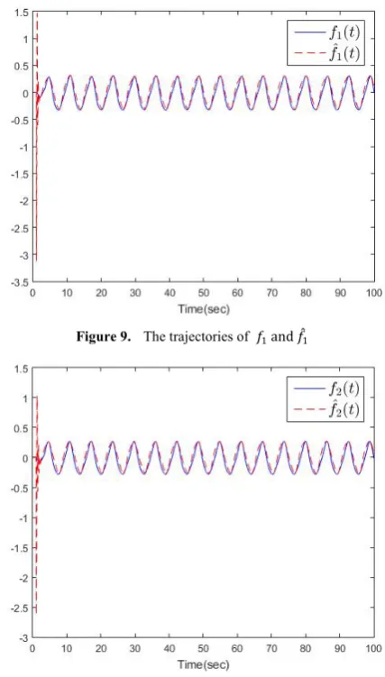
sliding mode controller. Moreover, the unknown system functions can be approximated well based on the proposed adaptive laws.
Remark 2: In this paper, the time delay, the state estimator, and input saturation are considered simultaneously, which are different from the previous literature [6] and [8].
Figure 6. The first-level sliding surface 𝑠𝑠1= 𝑐𝑐1𝑒𝑒1+ 𝑒𝑒̇1
Figure 7. The first-level sliding surface 𝑠𝑠2= 𝑐𝑐2𝑒𝑒2+ 𝑒𝑒̇2
Figure 8. The second-level sliding surface S = 𝛼𝛼1𝑠𝑠1+ 𝛼𝛼2𝑠𝑠2
Figure 9. The trajectories of 𝑓𝑓1 and 𝑓𝑓̂1
Figure 10. The trajectories of 𝑓𝑓2 and 𝑓𝑓̂2
5. Conclusions
REFERENCES
[1] L. Wu, W. Luo, Y. Zeng, F. Li, and Z. Zheng, “Fault detection for underactuated manipulators modeled by markovian jump systems,” IEEE Transactions on Industrial Electronics, vol. 63, no. 7, pp. 4387-4399, Jul. 2016.
[2] X. Lai, Y. Wang, M. Wu, and W. Cao, “Stable control strategy for planar three-link underactuated mechanical system,” IEEE/ASME Transactions on Mechatronics, vol. 21, no. 3, pp. 1345-1356, Jun. 2016.
[3] Z. H. Zhang and G. H. Yang, “Time-varying threshold-based fault detection for a class of uncertain non-linear systems in strict-feedback form,” IET Control Theory & Applications, vol. 10, no. 17, pp. 2149-2159, Nov. 2016.
[4] H. Zargarzadeh, T. Dierks, and S. Jagannathan, “Optimal control of nonlinear continuous-time systems in strict-feedback form,” IEEE Transactions on Neural Networks and Learning Systems, vol. 26, no. 10, pp. 2535-2549, Oct. 2015.
[5] B. Xu, Z. Shi, C. Yang, and F. Sun, “Composite neural dynamic surface control of a class of uncertain nonlinear systems in strict-feedback form,” IEEE Transactions on Cybernetics, vol. 44, no. 12, pp. 2626-2634, Dec. 2014. [6] M. Chen, G. Tao, and B. Jiang, “Dynamic surface control
using neural networks for a class of uncertain nonlinear systems with input saturation,” IEEE Transactions on Neural Networks and Learning Systems, vol. 26, no. 9, pp. 2086-2097, Sep. 2015.
[7] W. Liu, J. Lu, Z. Zhang, and S. Xu, “Observer-based neural control for MIMO pure-feedback non-linear systems with input saturation and disturbances,” IET Control Theory & Applications, vol. 10, no. 17, pp. 2314-2324, Nov. 2016.
[8] L. Long and J. Zhao, “Adaptive fuzzy output-feedback control for switched uncertain non-linear systems,” IET Control Theory & Applications, vol. 10, no. 7, pp. 752-761, Apr. 2016.
[9] Y. Li and S. Tong, “Adaptive fuzzy output-feedback stabilization control for a class of switched nonstrict-feedback nonlinear systems,” IEEE Transactions on Cybernetics, vol. 47, no. 4, pp. 1007-1016, Apr. 2017.
[10] L. X. Wang, A course in fuzzy systems and control,
Englewood Cliffs, NJ: Prentice-Hall, 1997.
[11] C. C. Kung and T. H. Chen, “Observer-based indirect adaptive fuzzy integral sliding mode control with state variable filters,” Fuzzy Sets and Syst., vol. 155, no. 2, pp. 292–308, 2005.
[12] Z. Zhu, Y. Xia, and M. Fu, "Adaptive sliding mode control for attitude stabilization with actuator saturation," IEEE Transactions on Industrial Electronics, vol. 58, no. 10, pp. 4898-4907, Oct. 2011.
[13] J. H. Park and G. T. Park, “Adaptive fuzzy observer with minimal dynamic order for uncertain nonlinear systems,” IEE Proc. Theory & Applications, vol. 150, no. 2, pp. 189-197, 2003.