A High Order Compact ADI Method for Solving 3D Unsteady Convection Diffusion Problems

http://www.sciencepublishinggroup.com/j/acm doi: 10.11648/j.acm.20180701.11

ISSN: 2328-5605 (Print); ISSN: 2328-5613 (Online)

A High Order Compact ADI Method for Solving 3D Unsteady

Convection Diffusion Problems

Yongbin Ge, Fei Zhao, Jianying Wei

*

Institute of Applied Mathematics and Mechanics, Ningxia University, Yinchuan, China

Email address:

[email protected] (Jianying Wei)

*_{Corresponding author}

To cite this article:

Yongbin Ge, Fei Zhao, Jianying Wei. A High Order Compact ADI Method for Solving 3D Unsteady Convection Diffusion Problems. Applied and Computational Mathematics s. Vol. 7, No. 1, 2018, pp. 1-10. doi: 10.11648/j.acm.20180701.11

Received: December 3, 2017; Accepted: December 13, 2017; Published: January 12, 2018

Abstract:

In this paper, we develop a rational high order compact alternating direction implicit (RHOC ADI) method for solving the three dimensional (3D) unsteady convection diffusion equation. The present scheme, based on the idea of the fourth order rational compact finite difference operator for the spatial discretization and the Crank-Nicolson method for the time discretization, is fourth order accurate in space and second order accurate in time. The solution procedure consists of a number of tridiagonal matrix operations, which makes the computation to be cost-effective. It is shown by means of the discrete Fourier analysis that this method is unconditionally stable. Three test problems are given to demonstrate the performance of the present method. The numerical results show that the present RHOC ADI scheme has higher accuracy and better phase and amplitude error characteristics than the classical second order Douglas-Gunn ADI method [16] and some high order compact ADI methods including the Karaa’s HOC ADI method [26], Cao and Ge’s HOC ADI method [27], and our previous exponential HOC ADI method [28]

.

Keywords:

3D Unsteady Convection Diffusion Equation, Rational, High Order Compact Scheme, ADI Method, Stability

1. Introduction

In this paper, we consider the following 3D unsteady convection diffusion equation:

2 2 2

2 2 2 ( , , , )

u u u u u u u

a b c p q r S x y z t

t x y z x y z

∂ ₋ ∂ ₋ ∂ ₋ ∂ ₊ ∂ ₊ ∂ ₊ ∂ ₌

∂ ∂ ∂ ∂ ∂ ∂ ∂

( , , , )x y z t ∈ Ω ×(0, ]T (1)

is unknown function in a cubic domain _Ω with initial condition

0

( , , , 0) ( , , ), ( , , )

u x y z =u x y z x y z ∈ Ω, (2)

and Dirichlet boundary condition

( , , , ) ( , , , ), ( , , , ) (0, ]

u x y z t =g x y z t x y z t ∈ ∂Ω × T (3)

where ∂Ω is the boundary of Ω, and u₀, g and the

source termSare given functions with sufficient smoothness. In Eq. (1), a , b and c are nonnegative diffusion coefficients and p, q and r _{are convective coefficients in}

the x-, y- and z-direction, respectively. The convection diffusion equation (1) is one of the most important models of mathematical physics, which may be considered as a simplified version of the Navier-Stokes equations and plays a very important role in computational fluids dynamics. It also can be seen in many applications to model the convection and diffusion of various physical quantities, such as mass, momentum, energy, vorticity, etc. [1-3].

Finite difference methods have been widely used to solve unsteady convection diffusion equations [4-28]. Among them, traditional numerical discretization schemes, such as the classical explicit difference scheme (forward difference for time and central difference for space), the classical implicit difference scheme (backward difference for time and central difference for space), and explicit or implicit upwind difference schemes, are either first order or second order accurate in space, and get poor solutions for convection-dominated problems if the mesh is not sufficiently refined. In general, explicit ( , , , )

difference schemes usually have a small stability region, which would lead the schemes diverge if the stability conditions are not satisfied. So, very small temporal step size must be chosen to keep computation converge. On the other hand, fully implicit difference schemes show good stability, and relatively big temporal step size can be used. But to get a solution of a large linear system arising from an implicit scheme at each time step, direct methods based on Gaussian elimination or conventional iterative methods, such as Gauss-Seidel, Jacobi, and SOR etc. may be too expensive to be used in practice, especially for higher dimensions.

To overcome these difficulties, there exist at least two alternative strategies. One is to use high order finite difference methods [4-14, 17-23, 25-28]. In the last few years, implicit high order compact difference schemes for solving 1D and 2D unsteady convection diffusion equations have been developed [5-10, 12-14]. These schemes usually have third to fourth order accuracy in space and have a large stability region [5, 8, 10], and they are even unconditionally stable [7, 12, 13]. With relatively big temporal step size, they can obtain much more accurate solutions than the classical difference schemes. However, traditional iterative methods still be used to solve the sparse linear system arising from the implicit difference schemes at each time step [5, 10]. Biconjugate gradient stabilized method (BiCGStab) is used in [13, 14]. This method is more efficient than conventional iterative methods, such as Gauss-Seidel, Jacobi, and SOR etc. However, it is still expensive to be used at each time step, especially for higher dimensional problems. The other strategy is to develop efficient and cost-effective difference algorithms, such as alternating direction implicit (ADI) [11, 15, 16, 18, 20-23, 25-28] or locally one dimensional (LOD) procedures [29-32], which are based on reducing high dimensional problems in several space variables to collections of 1D problems and only requiring to solve tridiagonal matrices, are simple to implement and economical to use. It is well known that the classical ADI method developed by Peaceman and Rachford [15], and Douglas and Gunn [16] have been popular due to their computational cost-effectiveness. However, these two ADI schemes, which are second order accurate in space and often produce significant dissipation and phase error [11, 21, 22], are not ideally suited to deal with the spatial discretization of convection-dominated transport problems. And the Peaceman-Rachford ADI scheme for 3D convection diffusion problems is conditionally stable. To achieve higher spatial accuracy computational cost-effectiveness, recently, there has been a renewed interest in the development of HOC ADI methods for 2D and 3D unsteady convection diffusion equations. Karra and Zhang [20], You [21], Tian and Ge [22], Tian [11], developed, respectively, an HOC ADI method for

solving 2D unsteady convection diffusion equations with constant coefficients. They are all second order accurate in time, fourth order accurate in space and unconditionally stable. Very recently, Sun and Li [23] presented a combined compact difference ADI (CCD ADI) method for solving 2D unsteady convection diffusion equations. This method is second order accurate in time, sixth order accurate in space and unconditionally stable. For 3D unsteady convection diffusion problems, Wang and Shen [25] proposed two splitting schemes, which are fourth order accurate for spatial diffusion term and second order accurate in time and a revised ADI scheme which obtains spatial fourth order accurate for convective term. Karaa [26] derived a so called delta formulation of HOC ADI (DHOC ADI) scheme, which is second order accurate in time and fourth order accurate in space. It is shown by using a discrete Fourier analysis that the method is unconditionally stable in the diffusion case. However, it is conditionally stable in the convection diffusion case. Recently, Cao and Ge [27] extended Karra and Zhang’s HOC ADI scheme [20] to the 3D case. Ge et al. [28] extended Tian and Ge’s EHOC ADI scheme [22] to the 3D case. These two generalized HOC ADI schemes are second order accurate in time, fourth order accurate in space and unconditionally stable. More recently, finite difference method is also employed by some authors to solve multidimensional unsteady convection diffusion reaction equations [35, 36].

Among these HOC ADI schemes, Tian [11] proposed a rational HOC ADI (RHOC ADI) scheme for solving the 2D unsteady convection diffusion problems, which is temporally second order, spatially fourth order and unconditionally stable. The main advantage of the RHOC ADI scheme is that it is more accurate than the existing other HOC ADI schemes, such as Karra and Zhang [20], You [21], Tian and Ge [22]. So, in this article, we are aiming at developing an RHOC ADI to solve the 3D unsteady convection diffusion equation. This paper is organized as follows. Section 2 presents the RHOC ADI finite difference method for the 3D unsteady convection diffusion problems; in Section 3, the Fourier (or von Neumann) stability analysis is used to show that the proposed RHOC ADI method is unconditionally stable in the convection diffusion case; in Section 4, numerical experiments for three test problems are performed to validate the effectiveness of the present schemes; finally, Section 5 is devoted to some conclusion.

2. Rational High Order Compact ADI

Scheme

For convenience of deduction, Eq. (1) is rewritten as:

2 2 2

2 2 2 ( , , , )

u u u u u u u

a b c p q r S x y z t

x y z t

x y z

∂ ∂ ∂ ∂ ∂ ∂ ∂

− − − + + + = −

∂ ∂ ∂ ∂

∂ ∂ ∂ (4)

We introduce the basic idea of rational high order compact ADI method by using the 1D steady convection diffusion equation as following

( )

xx x

au pu f x

where a _{is the nonnegative constant conductivity,} p _is

the constant convective velocity, and f x( ) is a sufficiently smooth function of x. Using the technique outlined in [11], we can easily derive a three-point fourth order compact scheme for Eq. (5), which is formulated symbolically as

1 4

( )

x x i i x

L A u− = +f O h (6)

in which

2

1 2

1

x x x

L = +α δ +α δ , Ax= −αδx2+pδx (7)

and δx and δx2 are the second order central difference

operators for the first and second derivatives respectively, hx

is the mesh size in the x-direction, and the coefficients α1, 2

α and α are given as follows:

1 , 0 0, 0 a p p p α α −  ≠  =  ₌  , 2 2 2 2 ( ) , 0 6 , 0 12 x x h a a p p h p α α  ₋ + ≠   =  =   , 2 4 2 4 1 12 144 1 6 36 x x x x Pe Pe a Pe Pe α   − +     =   − +     (8)

where Pex is the cell Reynolds number in the x-direction

and Pex = phx a. It is obvious that Eq. (6) with Eqs. (7)

and (8) is a fourth order scheme for convection diffusion equation (5). This scheme is named as an RHOC difference scheme in [11]; i.e., the influencing coefficients of the difference scheme formulation are connected to the rational functions of the coefficients of the differential operators and mesh size.

For convenience, we define the fourth order finite difference operators about y-and z-direction as follows:

2

1 2

1

y y y

L = +

β δ

+

β δ

, Ay = −

βδ

y2+q

δ

y, (9)

2

1 2

1

z z z

L = +γ δ +γ δ , Az = −γδz2+rδz, (10)

and δy, δ_z,

δ

_y2 and δ_z2 are the second order central

difference operators for the first and second derivatives, hy

and hz are the mesh size in the y- and z-direction,

respectively, and the coefficients β1, β2,

β

, γ1, γ2 and

γ _{are given as follows:}

1 , 0 0, 0 b q q q β β −  ≠  =  ₌  , 2 2 2 2 ( ) , 0 6 , 0 12 y y h b b q q h q

β

β

 ₋  _{+ ≠}  =  =   , 2 4 2 4 1 12 144 1 6 36 y y y y Pe Pe b Pe Pe β    _{− +}    = _{ }  _{− +}    (11) 1 , 0 0, 0 c r r r γ γ −  ≠  =  ₌  , 2 2 2 ₂ ( ) , 0 6 , 0 12 z z h c c r r h r γ γ  ₋ + ≠   =  =  , 2 4 2 4 1 12 144 1 6 36 z z z z Pe Pe c Pe Pe γ   − +     =   − +     (12)

where Pey=qhy b, Pe_z =rh c_z .

Applying the rational fourth order compact difference operators L Ax1 x

−

, L A−y1 y and L Az1 z

−

to the 3D unsteady convection diffusion Eq. (4), it yields the following rational fourth order approximation

1 1 1 4 4 4

(L A_{x x} L A_{y y} L A u_{z z}) _ijkn (S u)_ijkn O h( _x h_y h_z)

t

− ₊ − ₊ − _{= −}∂ _{+ + +}

∂ (13)

Rearranging Eq. (13), we obtain

1 1 1 4 4 4

( u)n_ijk (L A_{x x} L A_{y y} L A u_{z z}) _ijkn S_ijkn O h( _x h_y h_z)

t

− − −

∂

− = + + − + + +

∂ (14)

In which ijk represents the spatial position of ( ,x yi j,zk) and u_ijkn represents the approximate solution at time level

n

t = ∆n t, n _{represents the temporal level, and} n 1 n

t t + t

∆ = − is the temporal step size.

It is easy to see that Eq. (13) is fourth order semidiscrete approximation to the 3D unsteady convection diffusion Eq. (1). In the following, n

u and n

S will be written in short for uijkn and n ijk

application of the forward Taylor series expansion, we have

2 3

1 2 3

2 3

1 1

(1 ) exp( )

2! 3! ⋯

n n n

u t t t u t u

t t t t

+ _{= + ∆} ∂ _{+ ∆} ∂ _{+ ∆} ∂ _{+ = ∆} ∂

∂ ∂ ∂ ∂ (15)

whose equivalent equation is

1

exp( ) exp( )

2 2

n n

t t

u u

t t

+

∆ ∂ ∆ ∂

− =

∂ ∂ (16)

Combining Eq. (16) with Eq. (14), a fourth order difference approximation of Eq. (1) is obtained by

(

1 1 1 1 1

)

exp ( )

2

n n

x x y y z z

t

L A− L A− L A u− + S +

∆

 

+ + −

 

 

(

)

1 1 1

exp ( )

2

n n

x x y y z z

t

L A− L A− L A u− S

∆

 

= − + + − 

  (17)

Under the assumptions of the constant convective and diffusive coefficients, the difference operators Ax, Ay, A_z, L_x, y

L _and z

L commute with each other, which yields that

1 1 1 1 1

exp( ) exp( ) exp( ) exp( )

2 2 2 2

n n

x x y y z z

t t t t

L A− L A− L A u− + S +

∆ ∆ ∆ ₋∆

1 1 1

exp( ) exp( ) exp( ) exp( )

2 2 2 2

n n

x x y y z z

t t t t

L A− L A− L A u− S

∆ ∆ ∆ ∆

= − − − (18)

By using the Taylor expansions, and rearranging it, we have

1 1 1 1

(1 )(1 )(1 )

2 2 2

n

x x y y z z

t t t

L A− L A− L A u− +

∆ ∆ ∆

+ + +

1 1 1 1

(1 )(1 )(1 ) ( )

2 2 2 2

n n n

x x y y z z

t t t t

L A− L A− L A u− S + S

∆ ∆ ∆ ∆

= − − − + +

3 4 4 4

( ) ( x y z)

O t O th th th

+ ∆ + ∆ + ∆ + ∆ (19)

When applied to both sides of Eq. (19) with the difference operator L L Lx y z and neglected O(∆ + ∆t3) O( thx4+ ∆thy4+ ∆thz4), it

becomes

1

( )( )( )

2 2 2

n

x x y y z z

t t t

L +∆ A L +∆ A L +∆ A u +

1

( )( )( ) ( )

2 2 2 2

n n n

x x y y z z x y z

t t t t

L ∆ A L ∆ A L ∆ A u ∆ L L L S + S

= − − − + + (20)

It is clear that the approximation (20) is fourth order accurate in space and second order accurate in time, and has a compact 27-point stencil. It involves only discrete difference operators of the form 1

x

ω

δ , 2

y ω

δ or 3 z ω

δ , where ω1, ω2 and ω3 are

nonnegative integers less than or equal to 2. Finally, we introduce two intermediate variables _u* _and **

u , and apply the D’Yakonov ADI-like scheme [33], then we can get the following RHOC ADI scheme for the 3D unsteady convection diffusion equation with a source term.

** 1

* **

1 *

( ) ( )( )( ) ( )

2 2 2 2 2

( )

2

( )

2

n n n

x x x x y y z z x y z

y y

n

z z

t t t t t

L A u L A L A L A u L L L S S

t

L A u u

t

L A u u

+

+

∆ ∆ ∆ ∆ ∆



+ = − − − + +

 

∆



+ =

 

∆



+ =

 

(21)

the RHOC ADI scheme (21) can be computed by applying the 1D tridiagonal Thomas algorithm with a considerate saving in computing time. The intermediate variable values of _u* _{and u}** _{at the boundaries in the first and second} ADI scheme above are explicitly given in terms of the central difference of _gn+1 _{with respect to y and z from Eq. (2)}

and Eq. (3).

* 1

( )

2 n

z z

t

u = L +∆ A g + (22)

** _{( )( )} 1

2 2

n

y y z z

t t

u = L +∆ A L +∆ A g + (23)

3. Stability Analysis

In the following, we use the Fourier (or von Neumann) method for linear stability analysis of the RHOC ADI scheme (21). Let the numerical solution be expressed by means of a Fourier series, whose typical term is

exp{ }exp{ }exp{ }

n n

ijk x y z

u =

ξ

I

σ

i I

σ

j I

σ

k . (24)

where I= −1 , ξn is the amplitude at time level n,

, ,

i x j y k z

x =ih y = jh z =kh _{, and} σx(=θx xh ), σy(=θy yh ) and

( )

z z zh

σ =θ are phase angles with the wave numbers θx, θy

and θz in the x-, y- and z-direction, respectively.

Substituting the discrete Fourier mode (24) in both sides of Eq. (20), we can get the amplification factor

1 ( _x, _y, _z) n / n

Gσ σ σ =ξ + ξ , as follows:

( _x, _y, _z) _x( _x) _y( _y) _z( _z)

Gσ σ σ =g σ g σ g σ ₍₂₅₎

where g_x(θ_x) is given by

1 2 3 4

1 2 3 4

( ) ( )

( )

( ) ( )

x x

I g

I

η η η η

σ

η η η η

− + −

=

+ + + (26)

with

2 2

1 ₂

4

1 sin

2 x

x h

σ

α

η

= − , 2 ₂ 2

2 sin

2 x

x t h

σ

α

η

= ∆ , 3 1sin x

x h

α

η

=

σ

, 4 sin

2 _x x

p t h

η = ∆ σ (27)

In the same way, we can obtain the other two terms gy(σy)

and gz(σz) by replacing x by y and z, p by q and

r, α by β and γ , α1 by β1 and γ1, α2 by β2

and γ2 in the above expressions, respectively. It was proved that gx(σx)≤1 for all θx∈ −[ π π, ] in [11]. Similar conclusions can be drawn for gy(σy) and g_z(σ_z), that is

( ) 1

y y

g σ ≤ and g_z(σ_z) ≤1 . Therefore, the present RHOC ADI method, when applied to the 3D unsteady convection diffusion problems, is unconditionally stable.

4. Numerical Experiments

In this section, three test problems possessing exact solutions are given to demonstrate the performance of the RHOC ADI method. We compare the numerical results of the

present method with those of the Douglas-Gunn ADI scheme [16], the Karaa’s DHOC ADI schemes [26], Cao and Ge’s PHOC ADI scheme [27] and EHOC ADI scheme developed by Ge at al. [28]. We conduct our computations using double precision arithmetic on P4/3.4G dual-core personal computer with 4GB memory.

4.1. Problem 1

We first consider a 3D unsteady diffusion problem in the unit cubic region

[ ] [ ] [ ]

0,1× 0,1× 0,1 , with the coefficients

1

a= = =b c , p= = =q r 0_{, and}

2 2

( , , , ) 2 exp( ) sin( ) sin( ) sin( )

S x y z t = π −π t πx πy πz

so that the analytical solution is given by 2

( , , , ) exp( ) sin( ) sin( ) sin( )

u x y z t = −π t πx πy πz

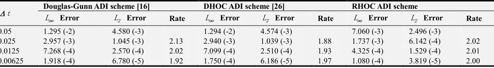
Table 1. L∞ and L∞ norm errors and convergence rate at ∆ =t h2, T=0.2, Problem 1.

h Douglas-Gunn ADI scheme [16] DHOC ADI scheme [26] RHOC ADI scheme ∞

L Error L2 Error Rate L∞ Error L2 Error Rate L∞ Error L2 Error Rate

1/5 1.291 (-2) 5.307 (-3) 6.943 (-3) 2.853 (-3) 3.976 (-3) 1.634 (-3)

1/10 2.148 (-3) 7.595 (-4) 2.80 4.600 (-4) 1.626 (-4) 4.13 2.850 (-4) 1.008 (-4) 4.02

1/20 4.488 (-4) 1.587 (-4) 2.26 2.830 (-5) 1.000 (-5) 4.02 1.780 (-5) 6.293 (-6) 4.00

1/40 1.068 (-5) 3.777 (-5) 2.07 1.762 (-6) 6.231 (-7) 4.00 1.112 (-6) 3.933 (-7) 4.00

Table 2. L∞ and L∞ norm errors and convergence rate at h=0.01, T=0.2, Problem 1.

Δt Douglas-Gunn ADI scheme [16] DHOC ADI scheme [26] RHOC ADI scheme

∞

L Error L2 Error Rate L∞ Error L2 Error Rate L∞ Error L2 Error Rate

0.05 1.295 (-2) 4.580 (-3) 1.294 (-2) 4.574 (-3) 7.060 (-3) 2.496 (-3)

The initial and Dirichlet boundary conditions are directly taken from this analytical solution. This test problem was used in [26-28]. For the 3D pure diffusion equation, the PHOC ADI scheme, the EHOC ADI scheme and the present RHOC ADI scheme are the same, because, actually, they all reduce to the standard fourth order Padé scheme. So, we just use the Douglas-Gunn ADI scheme, the DHOC ADI scheme, and the present RHOC ADI scheme to compute. We consider uniform grids (h=hx=hy=hz) with different mesh sizes.

The compared quantities are the L_∞ norm errors, L2 norm errors and convergence rate of the numerical solution with respect to the exact solution. The rate of convergence is defined by ln (2 err1 /err2), where err1 and err2 are the

2

L norm errors with the spatial grid sizes h and h/ 2 or temporal grid sizes ∆t and ∆t/ 2, respectively.

In Table 1, we set _{∆ =t h}2_{, T} =_{0.2 and halve the spatial} grid sizes h from 1/ 5 to 1/ 40 to demonstrate the spatial fourth order accuracy. We see that the present RHOC ADI and the DHOC ADI schemes are fourth order accurate in

space, whereas the Douglas-Gunn ADI scheme is second order accurate in space. The present RHOC ADI scheme provides more accurate solution than the Douglas-Gunn ADI scheme or the DHOC ADI scheme. In Table 2, h=0.01,

0.2

T = and the change of temporal grid sizes ∆t from 0.05 to 0.00625 are chosen for the demonstration of temporal second order accuracy. We observe that all three schemes have second order accuracy in time. However, the results of the present RHOC ADI scheme and the DHOC ADI scheme become more and more accurate with the reduction in time step than the ones of the Douglas-Gunn ADI scheme.

4.2. Problem 2

To further study the performance of the present RHOC ADI scheme, we apply it to a 3D unsteady convection diffusion problem which is defined in the unit cubic region

[ ] [ ] [ ]

0, 2 × 0, 2 × 0, 2 , with an exact solution given, as in [26-28], by

3 2 2 2

2 ( 0.5) ( 0.5) ( 0.5)

( , , , ) (4 1) exp

(4 1) (4 1) (4 1)

x pt y qt z rt

u x y z t t

a t b t c t

−  _{− − − − − −} 

= + _− − − _

+ + +

 

The Dirichlet boundary and initial conditions are set to satisfy this exact solution.

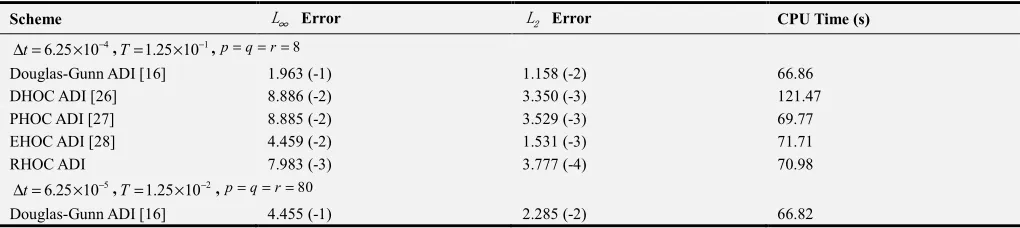
In Table 3, the L_∞ norm errors, the L₂ norm errors and the CPU time are shown by using the present RHOC ADI, the Douglas-Gunn ADI [16], the DHOC ADI [26], the PHOC ADI [27], and the EHOC ADI [28] schemes. We fix

0.01

a= = =b c and h=h_x=h_y =h_z =0.025 _{, change}

p= =q r _{from 8 to 8000 , ∆t from} 4 6.25 10× − to 7

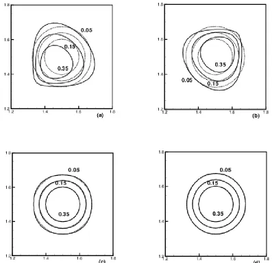
6.25 10× − , and T from _{1.25 10×} −1 _{to 1.25 10×} −4 _{. The} results in Table 3 show that the present RHOC ADI scheme provides a higher accuracy solution than the Douglas-Gunn ADI scheme and the other HOC ADI schemes. We notice the DHOC ADI scheme is divergent when convective coefficients are larger than a certain number. There is nothing strange since the DHOC ADI scheme is conditionally stable for the convection diffusion problem [26]. In Figure 1, 4

6.25 10

t −

∆ = × , 0.125

T = , p= = =q r 8 , a= = =b c 0.01 ,1.2≤x y, ≤1.8 _,

1.5

z = , and h=0.025 are chosen for comparison of the Douglas-Gunn ADI (a), the DHOC ADI (b), the EHOC ADI (c), and the present RHOC ADI (d) schemes with the exact

solution. It shows that under this condition, the present RHOC ADI scheme is the most accurate, whereas the Douglas-Gunn ADI scheme, the DHOC ADI scheme, and the EHOC ADI scheme, are not so accurate. For further comparison, we set

6

10

25

.

6

×

−

=

∆

t

, T =0.00125, p=q=r=800,

, 8 . 1 , 2 .

1 ≤x y≤ z=1.5, h=0.025 in Figure 2. We also notice that the present RHOC ADI scheme can still give much better results than the other HOC ADI schemes. This fact can also be seen by observing the position of contour plots of solution surface. An analysis of Figure 1 and Figure 2 shows that the present RHOC ADI scheme produces a numerical solution in good agreement with the exact solution. However, noticeable phase differences are observed between the other HOC ADI schemes and the exact solution. We also notice that the RHOC ADI, the PHOC ADI, the EHOC ADI and the Douglas-Gunn ADI methods exhibit less CPU time than that of the DHOC ADI method from Table 3. The execution CPU time of the RHOC ADI method is much less than that of the DHOC ADI method. This clearly shows that the RHOC ADI method is the most effective in view of accuracy and time consumption.

Table 3. L∞and L norm errors and CPU time of five ADI scheme with 2 h=0.025, Problem 2.

Scheme L∞ Error L2 Error CPU Time (s)

4

6.25 10

t −

∆ = × ,_{T=1.25 10×} −1_,p= = =_{q r 8}

Douglas-Gunn ADI [16] 1.963 (-1) 1.158 (-2) 66.86

DHOC ADI [26] 8.886 (-2) 3.350 (-3) 121.47

PHOC ADI [27] 8.885 (-2) 3.529 (-3) 69.77

EHOC ADI [28] 4.459 (-2) 1.531 (-3) 71.71

RHOC ADI 7.983 (-3) 3.777 (-4) 70.98

5

6.25 10

t −

∆ = × ,_{T=1.25 10×} −2_{,p= = =q r 80}

Scheme L∞ Error L2 Error CPU Time (s)

DHOC ADI [26] 3.010 (-1) 1.223 (-2) 121.01

PHOC ADI [27] 3.018 (-1) 1.223 (-2) 69.72

EHOC ADI [28] 1.375 (-1) 3.782 (-3) 71.66

RHOC ADI 2.674 (-2) 9.888 (-4) 70.92

6

6.25 10

t −

∆ = × ,_{T=1.25 10×} −3_{,p= = =q r 800}

Douglas-Gunn ADI [16] 4.874 (-1) 2.470 (-2) 66.78

DHOC ADI [26] 1.477 (+20) 5.924 (+19) 119.61

PHOC ADI [27] 3.248 (-1) 1.411 (-2) 69.68

EHOC ADI [28] 1.567 (-1) 4.199 (-3) 70.62

RHOC ADI 3.137 (-2) 1.115 (-3) 70.87

7

6.25 10

t −

∆ = × , _{T=1.25 10×} −4_{,p= = =q r 8000}

Douglas-Gunn ADI [16] 4.918 (-1) 2.490 (-2) 66.74

DHOC ADI [26] 1.918 (+24) 1.130 (+24) 119.38

PHOC ADI [27] 3.267 (-1) 1.433 (-2) 69.64

EHOC ADI [28] 1.588 (-1) 4.244 (-3) 70.57

RHOC ADI 3.189 (-2) 1.129 (-3) 70.82

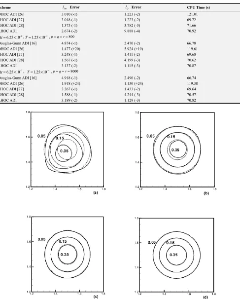
Figure 1. Contour lines (0.05, 0.15 and 0.35) of the pulse: Douglas-Gunn ADI scheme and exact (a), DHOC ADI scheme and exact (b), EHOC ADI scheme and exact (c), and RHOC ADI scheme and exact (d), in the subregion 1.2≤x y, ≤1.8, on z=1.5 at ∆ =t 6.25 10× −4, T=0.125, p= = =q r 8, a= = =b c 0.01,

0.025

Figure 2. Contour lines (0.05, 0.15 and 0.35) of the pulse: Douglas-Gunn ADI scheme and exact (a), PHOC ADI scheme and exact (b), EHOC ADI scheme and exact (c), and RHOC ADI scheme and exact (d), in the subregion 1.2≤x y, ≤1.8, on z=1.5 at ∆ =t 6.25 10× −6,T=0.00125, p= = =q r 800 ,

0.01

a= = =b c ,h=0.025. Dot contour lines in (a) - (d) correspond to exact solution.

4.3. Problem 3

We consider a 3D unsteady pure convection problem which is defined with the periodic boundary condition in the unit cubic region

[ ] [ ] [ ]

0, 2 × 0, 2 × 0, 2 . The initial conditions is given by

( , , , 0) sin( ( ))

u x y z =

π

x+ +y z

This problem is revised by the 2D pure convection problem considered in [11, 34], which was used as a test

problem of a sin-surface periodic flow. For this problem, the DHOC ADI, the PHOC ADI, and the EHOC ADI schemes become singular because a= = =b c 0, so these three HOC ADI schemes cannot be used. We just use the present RHOC ADI and the Douglas-Gunn ADI schemes to compute the numerical solution of this problem. The compared quantities are the L_∞ and L2 norm errors and convergence rate of the numerical solution with respect to the exact solution.

Table 4. L_∞ and L_∞ norm errors and convergence rate at _{∆ =t h}2_,

0.2

T= , Problem 3.

h Douglas-Gunn ADI Scheme [16] RHOC ADI Scheme

∞

L Error L2 Error Rate L∞ Error L2 Error Rate

0.2 0.862 5.216 (-1) 1.418 (-2) 8.403 (-3)

0.1 1.648 5.747 (-1) -0.14 9.310 (-4) 5.343 (-4) 3.98

0.05 3.354 7.375 (-1) -0.36 6.100 (-5) 3.380 (-5) 3.98

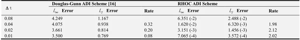
Table 5. L_∞ and L∞ norm errors and convergence rate at h=0.05, T=0.2, Problem 3.

Δt Douglas-Gunn ADI Scheme [16] RHOC ADI Scheme

∞

L Error L2 Error Rate L∞ Error L2 Error Rate

0.08 4.249 1.167 6.351 (-2) 2.488 (-2)

0.04 4.075 0.938 0.32 1.620 (-2) 6.320 (-3) 1.98

0.02 3.661 0.814 0.20 3.151 (-3) 1.456 (-3) 2.12

0.01 3.500 0.769 0.08 7.065 (-4) 3.572 (-4) 2.02

In Table 4, we set 2

t h

∆ = , T =0.2 and halve the spatial grid sizes h from 0.2 to 0.025 to qualify the spatial fourth order accuracy. We see that the results of the present RHOC ADI scheme become more and more accurate with the reduction in spatial step sizes, while the ones of the Douglas-Gunn ADI scheme are almost invariable. In Table 5, we fix h=0.05 and change ∆t from 0.08 to 0.01 to show the temporal accuracy order. We find that the present RHOC ADI scheme is second order accurate in time, whereas the Douglas-Gunn ADI scheme gives very poor solution.

5. Conclusion

In this article, a rational high order compact ADI method for solving the 3D unsteady convection diffusion equation is established. By using the fourth order compact method for spatial derivatives and using the second order Crank-Nicolson method for temporal derivative, the present RHOC ADI scheme is fourth order accurate in space, second order accurate in time and only involves three-point stencil for each 1D operator. So, in each ADI solution step, it can be solved by simple tridiagonal Gaussian decomposition and may be used by application of the 1D tridiagonal Thomas algorithm with a considerable amount of saving in computing time. It is shown by a discrete Fourier analysis that the RHOC ADI scheme is unconditionally stable. Numerical experiments for three test problems are performed to demonstrate its performance and to show its superiority over the classical Douglas-Gunn ADI scheme and the other existing HOC ADI schemes.

Acknowledgements

This work is supported in part by the National Natural Science Foundation of china under Grant 11361045 and 11772165.

References

[1] J. Bear, Dynamics of Fluids of Porous Media, American Elsevier Publishing Company, New York, 1972.

[2] S. V. Patankar, Numerical Heat Transfer and Fluid Flows, McGraw-Hill, New York, 1980.

[3] Z. Zlatev, R. Berkowicz, L. P. Prahm, Implementation of a variable stepsize variable formula method in the time-integration part of a code for treatment of long-range transport of air pollutants, J. Comput. Phys. 55 (1984) 278-301. [4] R. S. Hirsh, Higher order accurate difference solutions of fluid mechanics problems by a compact differencing technique, J.

Comput. Phys. 19 (1975) 90-109.

[5] B. J. Noye, H. H. Tan, Finite difference methods for solving the two-dimensional advection diffusion equation, Int. J. Numer. Meth. Fluids 9 (1988) 75-89.

[6] A. Rigal, High order difference schemes for one-dimensional convection-diffusion problems, J. Comput. Phys. 114 (1994) 59-76.

[7] K. W. Morton, Numerical Solution of Convection-diffusion Problems, Chapman & Hall, London, 1996.

[8] B. J. Noye, H. H. Tan, A third-order semi-implicit finite difference methods for solving the one-dimensional unsteady convection diffusion equation, Int. J. Numer. Meth. Eng. 26 (1998) 1615-1629.

[9] W. F. Spotz, G. F. Carey, Extension of high-order compact schemes to time-dependent problems, Numer. Meth. Partial Differential Eq.17 (2001) 657-672.

[10] J. C. Kalita, D. C. Dalal, A. K. Dass, A class of higher order compact schemes for the unsteady two-dimensional convection-diffusion equation with variable convection coefficients, Int. J. Numer. Meth. Fluids 38 (2002) 1111-1131. [11] Z. F. Tian, A rational high-order compact ADI method for

unsteady convection-diffusion equations, Comput. Phys. Commun. 182 (2011) 649-662.

[12] Z. F. Tian, P. X. Yu, A high-order exponential scheme for solving 1D unsteady convection- diffusion equations, J. Comput. Appl. Math. 235 (2011) 2477-2491.

[13] J. C. Kalita, S. Sen, An improved (9,5) higher order compact schemes for the transient two-dimensional convection-diffusion equation, Int. J. Numer. Meth. Fluids 51 (2006) 703 -717.

[14] J. C. Kalita, S. Sen, The (9,5) HOC formulation for the transient Navier-Stokes equations in primitive variable, Int. J. Numer. Meth. Fluids 55 (2007) 387-406.

[15] D. W. Peaceman, H. H. Rachford Jr., The numerical of parabolic and elliptic differential equations, J. Soc. Ind. Appl. Math. 3 (1959) 28-41.

[16] J. Douglas Jr., J. E. Gunn, A general formulation of alternating direction methods. I. Parabolic and hyperbolic problems, Numer. Math. 6 (1964) 428-453.

[17] M. Dehghan, A. Mohebbi, High-order compact boundary value method for the solution of unsteady convection-diffusion problems, Math. Comput. Simul.79 (2008) 683-699.

[18] J. Qin, The new alternating direction implicit difference methods for solving three-dimension parabolic equations, Appl. Math. Modelling, 34 (2010) 890-897.

[20] S. Karaa, J. Zhang, High order ADI method for solving unsteady convection-diffusion problems, J. Comput. Phys. 198 (2004) 1-9.

[21] D. You, A high-order Padé ADI method for unsteady convection-diffusion equations, J. Comput. Phys. 214 (2006) 1-11.

[22] Z. F. Tian, Y. B. Ge, A fourth-order compact ADI method for solving two-dimensional unsteady convection-diffusion problems, J. Comput. Appl. Math. 198 (2007) 268-286. [23] H. W. Sun, L. Z. Li, A CCD-ADI method for unsteady

convection-diffusion equations, Comput. Phys. Commun. 185 (2014) 790-797.

[24] M. Dehghan, Numerical solution of the three-dimensional advection-diffusion equation, Appl. Math. Comput. 150 (2004) 5-19.

[25] S. D. Wang, Y. M. Shen, Three high-order splitting schemes for 3D transport equation, Appl. Math. Mech. 26 (2005) 1007-1016.

[26] S. Karaa, A high-order compact ADI method for solving three-dimensional unsteady convection-diffusion problems, Numer. Meth. Partial Differential Eq. 22 (2006) 983-993. [27] F. Cao, Y. Ge. A high-order compact ADI scheme for the 3D

unsteady convection-diffusion equation. 2011 International Conference on Computational and Information Sciences. 2011, PP1087-1089.

[28] Y. Ge, Z. F. Tian, J. Zhang, An exponential high-order compact ADI method for 3D unsteady convection-diffusion problems, Numer. Meth. Partial Differential Eq. 29 (2013) 186-205.

[29] J. Qin, T. Wang, A compact locally one-dimensional finite difference method for nonhomogeneous parabolic differential equations, Int. J. Numer. Meth. Biomed. Engng. 7 (2011) 128-142.

[30] M. Dehghan, Implicit locally one-dimensional methods for two-dimensional diffusion with a non-local boundary condition, Math. Comput. Simulat. 49 (1999) 331-349.

[31] S. Karaa, An accurate LOD scheme for two-dimensional parabolic problems, Appl Math Comput, 170 (2005) 886-894. [32] W. Zhang, L. Tong, E. T. Chung, A new high accuracy locally one-dimensional scheme for the wave equation, J. Comput. Appl. Math. 236 (2011) 1343-1353.

[33] E. G. D’yakonov, Difference schemes of second-order accuracy with a splitting operator for parabolic equations without mixed derivatives, (Russian) Zh. Vychisl. Mat. I Mat. Fiz 4 (1964) 935-941.

[34] Y. Sun, Z. J. Wang, Evaluation of discontinuous Galerkin and spectral volume methods for scalar and system conservation laws on unstructured grids, Int. J. Numer. Meth. Fluids 45 (2004) 819-838.

[35] A. Kaya, Finite difference approximations of multidimensional unsteady convection-diffusion -reaction equations. J. Comput. Phys. 285 (2015) 331-349.