https://doi.org/10.5194/gmd-11-541-2018 © Author(s) 2018. This work is distributed under the Creative Commons Attribution 3.0 License.
Climate pattern-scaling set for an ensemble of 22 GCMs – adding
uncertainty to the IMOGEN version 2.0 impact system
Przemyslaw Zelazowski1,2, Chris Huntingford3, Lina M. Mercado3,4, and Nathalie Schaller1,5 1Oxford University Centre for the Environment, University of Oxford, Oxford, OX1 3QY, UK 2Centre of New Technologies, University of Warsaw, Warsaw, 02-097, Poland
3Centre for Ecology and Hydrology, Wallingford, OX10 8BB, UK
4Geography, College of Life and Environmental Sciences, University of Exeter, Exeter, EX4 4RJ, UK 5Center for International Climate Research (CICERO), Oslo, NO-0318, Norway
Correspondence:Chris Huntingford ([email protected])
Received: 22 August 2016 – Discussion started: 25 October 2016
Revised: 15 November 2017 – Accepted: 22 November 2017 – Published: 6 February 2018
Abstract. Global circulation models (GCMs) are the best tool to understand climate change, as they attempt to repre-sent all the important Earth system processes, including an-thropogenic perturbation through fossil fuel burning. How-ever, GCMs are computationally very expensive, which lim-its the number of simulations that can be made. Pattern scaling is an emulation technique that takes advantage of the fact that local and seasonal changes in surface climate are often approximately linear in the rate of warming over land and across the globe. This allows interpolation away from a limited number of available GCM simulations, to as-sess alternative future emissions scenarios. In this paper, we present a climate pattern-scaling set consisting of spatial cli-mate change patterns along with parameters for an energy-balance model that calculates the amount of global warming. The set, available for download, is derived from 22 GCMs of the WCRP CMIP3 database, setting the basis for simi-lar eventual pattern development for the CMIP5 and forth-coming CMIP6 ensemble. Critically, it extends the use of the IMOGEN (Integrated Model Of Global Effects of cli-matic aNomalies) framework to enable scanning across full uncertainty in GCMs for impact studies. Across models, the presented climate patterns represent consistent global mean trends, with a maximum of 4 (out of 22) GCMs exhibiting the opposite sign to the global trend per variable (relative humidity). The described new climate regimes are generally warmer, wetter (but with less snowfall), cloudier and windier, and have decreased relative humidity. Overall, when averag-ing individual performance across all variables, and without
considering co-variance, the patterns explain one-third of re-gional change in decadal averages (mean percentage variance explained, PVE, 34.25±5.21), but the signal in some models exhibits much more linearity (e.g. MIROC3.2(hires): 41.53) than in others (GISS_ER: 22.67). The two most often con-sidered variables, near-surface temperature and precipitation, have a PVE of 85.44±4.37 and 14.98±4.61, respectively. We also provide an example assessment of a terrestrial impact (changes in mean runoff) and compare projections by the IMOGEN system, which has one land surface model, against direct GCM outputs, which all have alternative representa-tions of land functioning. The latter is noted as an additional source of uncertainty. Finally, current and potential future ap-plications of the IMOGEN version 2.0 modelling system in the areas of ecosystem modelling and climate change impact assessment are presented and discussed.
1 Introduction
sea-sonal changes in surface climate are linear in terms of the rate of warming over land and across the globe. It allows interpo-lation away from a limited number of available GCM simu-lations, enabling a time-efficient assessment of surface mete-orological changes for alternative nonstandard future scenar-ios of changed GHG concentrations. This can include, for ex-ample, new scenarios that fall between the current represen-tative concentration pathways (RCPs, Taylor et al., 2012) and potentially the investigation of predefined future temperature thresholds such as 2◦C global warming above pre-industrial levels. Pattern scaling has been suggested as a key method-ology to understand the differences between climate stabil-isation at 1.5 and at 2.0◦C as well as the impacts of these scenarios (James et al., 2017).
Climate-change patterns (or “patterns”) are coefficients of the regression between areal mean warming over Earth’s land regions (1Tl, K) and local changes in surface climatol-ogy. They are derived by comparison against outputs from GCMs, and presented as local monthly mean changes over land per degree of mean warming over land. Pattern scaling is a simple procedure in which these patterns are multiplied by
1Tlto give local monthly changes in climatology. A global energy-balance model (EBM; e.g. Wigley et al., 2000) is ap-plied to model how the GHG concentrations translate into changes in radiative forcing (Q, W m−2) and then into tem-perature increase over land regions (1Tl).
The IMOGEN framework (Integrated Model Of Global Effects of climatic aNomalies; Huntingford et al., 2010) is a computationally efficient tool for modelling impacts of fu-ture climate change on terrestrial ecosystems. It consists of the JULES land surface model (Best et al., 2011; Clark et al., 2011) linked to a pattern-scaling module (Huntingford and Cox, 2000). The scaling provides monthly mean changes in climate variables over land, notably temperature, relative humidity, precipitation, shortwave and longwave radiation, wind speed, and pressure – quantities used to drive ecosys-tem models such as JULES. In addition, a simple oceanic global carbon cycle model is included (Joos et al., 1996 and Appendix of Huntingford et al., 2004), which expands the typical usage of pattern scaling by allowing consideration of oceanic climate–carbon cycle feedbacks, alongside land-based feedbacks. All simulations use an hourly time step and a spatial resolution of 2.5◦latitudinal×3.75◦longitudinal, or 72 by 96 grid boxes, as in the UKMO-HadCM3 GCM. Over land, but excluding Antarctica, this corresponds to 1631 grid boxes.
Linking forcings to mean warming over land, 1Tl, is achieved with the IMOGEN EBM which requires five pa-rameters (Huntingford and Cox, 2000, also listed in Sect. 2.2) which, as in the case of patterns, are also derived by fitting to GCM runs. These calibration parameters and the previously described patterns together form a “pattern-scaling set”.
IMOGEN was originally established to allow rapid assess-ment of a range of alternative GHG emission scenarios, e.g. corresponding to any standard Special Report on Emissions
Scenarios (SRESs, Naki´cenovi´c et al., 2000) or RCPS (Tay-lor et al., 2012), for which a GCM simulation is unavailable. IMOGEN, using its scaling patterns, enables interpolation away from the relatively few GCM simulations that do ex-ist towards new user-prescribed emissions or concentration pathways.
The general purpose of IMOGEN is to prescribe carbon dioxide (CO2) emissions, along with further prescription of non-CO2 radiative forcings for other GHGs and aerosols. From this, the model calculates evolving atmospheric CO2 concentrations as a consequence of driving CO2emissions. The related and also evolving overall radiative forcing Q
(W m−2) is calculated to drive the EBM. This has similarities to how GCMs have been forced with the SRESs in the third Coupled Model Intercomparison Project (CMIP3) archive, upon which this analysis is based. Alternatively, the full ra-diative forcingQcan be prescribed directly as a future forc-ing pathway, dependent on prescription of all atmospheric gas changes and in which case CO2concentrations are there-fore given. This has similarities to the more recent forcing of GCMs with RCPs, in part recognising that not all climate models have a fully interactive carbon cycle. RCPs were used to inform the fifth IPCC report (IPCC, 2013), via the set of climate model simulations available at that time in the CMIP5 dataset (Taylor et al., 2012). CMIP5 has evolved fur-ther since 2013 to hold more simulations; the exercise to cali-brate an EBM and derive climate patterns for CMIP5 is under way. In addition, the scientific community is now starting to consider a broader range of scenarios, named shared socioe-conomic pathways (SSPs) (Riahi et al., 2017), and these will drive the forthcoming CMIP6 (Eyring et al., 2016) simula-tions.
In practice, though, IMOGEN has been used much more to assess the effects of new parameterisations, adjustments or the inclusion of new processes into the JULES land sur-face model. This is as a precursor for any eventual place-ment of land surface model improveplace-ments in a full GCM. IMOGEN allows easy and fast assessment of ranges of pa-rameterisations, numerical stability checks and, critically, the relative importance of new understanding of ecological and hydrological responses globally, including feedbacks on the carbon cycle. Examples include the impacts of changes in diffuse radiation on the land carbon sink (Mercado et al., 2009), the effects of ozone damage on plant productivity (Sitch et al., 2007) and climate–carbon cycle feedbacks by permafrost melt (Burke et al., 2017).
of climate models. Such uncertainty can then be readily eval-uated against the magnitude of any further uncertainty in any terrestrial surface impacts of interest. In Sect. 2 we de-scribe the methods which lead to the pattern-scaling set. Sec-tion 3 describes the actual set, including discussion of inter-GCM differences. We include metrics describing the accu-racy of the linearity assumption of meteorological changes against level of global warming, as implicit in the scaling method. Section 4 reviews existing applications of the IMO-GEN pattern-scaling system and comments on the future general benefits of inclusion of climate model uncertainty in impacts assessments. Finally, Sect. 5 discusses the strengths and caveats of the pattern-scaling approach.
2 Data and methods
2.1 The WCRP CMIP3 multi-model dataset and data preprocessing
Spatial patterns (i.e. maps) of climate change and energy-balance model calibration parameters, together forming the “climate pattern-scaling set”, are derived from GCM data available through the World Climate Research Pro-gramme Coupled Model Intercomparison Project, phase three (WCRP CMIP3; Meehl et al., 2007a). The WCRP CMIP3 multi-model dataset resulted from an international effort to run a coordinated set of 20th- and 21st-century climate GCM simulations for a limited number of future scenarios, covering many aspects of climate variability and change. All these simulations were subsequently analysed and formed the basis of much that is reported in the Fourth Assessment (AR4) of the Intergovernmental Panel on Cli-mate Change (IPCC, 2007). The dataset consists of data from 24 GCMs, representing 17 modelling groups from 12 coun-tries. The climate pattern-scaling set presented here (Ta-ble 1) corresponds to 22 GCMs, because GISS_AOM is an atmosphere–ocean model without surface meteorologi-cal projections over land, and key data from CGCM3.1(T63) GCM were missing (see below). In the case of the GISS-EH and GISS-ER GCMs, WCRP CMIP3 data were supple-mented with the formally associated pool provided by Na-tional Aeronautics and Space Administration Goddard Insti-tute for Space Studies (http://data.giss.nasa.gov/pub/pcmdi). The analysed model runs represent scenarios of four types: (i) control experiments, which are either pre-industrial or present day (Picntrl or Pdcntrl; the codes are the file name conventions used in the WCRP database); (ii) the idealised 1 % yr−1CO2 increase up to doubled and quadrupled lev-els (1pctto2x, 1pctto4x); (iii) the 20th-century run (20C3M) representing modelled period from pre-industrial to present day; and (iv) the high-emission (A2) and mid-emission (A1B) future scenarios defined by the SRESs (Nakicenovic et al., 2000). When multiple simulations of any particular scenario are available, then the analysis is limited to the first
available, as the inter-run variability has been reported to be small (Frieler et al., 2012).
Variables analysed for each GCM are those representing monthly mean land surface climatology: 1.5 m air temper-ature (TAS), 1.5 m relative humidity (HURS), 10 m wind speed (UAS and VAS, combined into a directionless “UA”), precipitation (PR, including snow PRSN), downward short-wave (RSDS) and longshort-wave (RLDS) radiation fluxes and sur-face pressure (PS). The codes in brackets are the file name conventions used in the WCRP database for individual vari-ables. These seven variables are required to run the JULES land surface scheme inside the IMOGEN framework. Addi-tionally, net radiative flux at the top of the atmosphere (pos-itive downwards), Top of Model (RTMT), is also processed. This is required to drive the global energy-balance model.
There were some discrepancies between data requirements to run the IMOGEN system and the actual data availability in WCRP CMIP3. They are listed in Table 1. For all GCMs, surface relative humidity (HURS) data were not available, but a 4-D representation of this variable at predefined pres-sure levels (HUR) was generally available. This allowed ex-trapolation of surface relative humidity from the two nearest available pressure levels. In the case of INGV-SXG, PCM and CCSM3 GCMs, surface wind was obtained in the same procedure. For two cases, the required surface data were available, but suffered from quality and other issues. In the UKMO-HadGEM1 dataset, the last month of the SRES A2 simulation was missing (and in this study, it was filled in with interpolated values), and surface wind data were presented on a nonstandard grid (and it was interpolated onto a stan-dard UKMO-HadGEM1 grid). For MRI-CGCM2.3.2, many values in snow precipitation data (PRSN) were missing (the data were not used in this study) and there was no land mask available (SFTLF, later obtained from the Japanese mod-elling group). Additional details are given in Table 1.
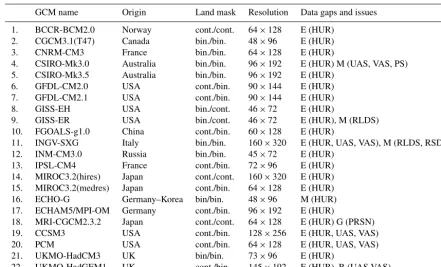
ap-Table 1.Availability of WCRP CMIP3 data for the climate patterns study, and characteristics of models’ depiction of land and water areas (variable sftlf). Land–water transition is either continuous (cont.) or abrupt (binary mask – bin.). The first characteristic in the column “Land mask” pertains to coastlines, whereas the second pertains to inland waters. The codes in column “Data gaps and issues” are as follows: M – missing, E – 4-D variable (surface values need to be extrapolated), G – data gaps, R – some data needed resizing.
GCM name Origin Land mask Resolution Data gaps and issues
1. BCCR-BCM2.0 Norway cont./cont. 64×128 E (HUR)
2. CGCM3.1(T47) Canada bin./bin. 48×96 E (HUR)
3. CNRM-CM3 France bin./bin. 64×128 E (HUR)
4. CSIRO-Mk3.0 Australia bin./bin. 96×192 E (HUR) M (UAS, VAS, PS)
5. CSIRO-Mk3.5 Australia bin./bin. 96×192 E (HUR)
6. GFDL-CM2.0 USA cont./bin. 90×144 E (HUR)
7. GFDL-CM2.1 USA cont./bin. 90×144 E (HUR)
8. GISS-EH USA bin./cont. 46×72 E (HUR)
9. GISS-ER USA bin./cont. 46×72 E (HUR), M (RLDS)
10. FGOALS-g1.0 China cont./bin. 60×128 E (HUR)
11. INGV-SXG Italy bin./bin. 160×320 E (HUR, UAS, VAS), M (RLDS, RSDS)
12. INM-CM3.0 Russia bin./bin. 45×72 E (HUR)
13. IPSL-CM4 France cont./bin. 72×96 E (HUR)
14. MIROC3.2(hires) Japan cont./cont. 160×320 E (HUR) 15. MIROC3.2(medres) Japan cont./bin. 64×128 E (HUR)
16. ECHO-G Germany–Korea bin/bin. 48×96 M (HUR)
17. ECHAM5/MPI-OM Germany cont./bin. 96×192 E (HUR)
18. MRI-CGCM2.3.2 Japan cont./cont. 64×128 E (HUR) G (PRSN)
19. CCSM3 USA cont./bin. 128×256 E (HUR, UAS, VAS)
20. PCM USA cont./bin. 64×128 E (HUR, UAS, VAS)
21. UKMO-HadCM3 UK bin/bin. 73×96 E (HUR)
22. UKMO-HadGEM1 UK cont./bin. 145×192 E (HUR), R (UAS,VAS)
plications of the IMOGEN tool, with 2.5◦latitudinal×3.75◦ longitudinal resolution. The common grid allows, in a sys-tematic way, to capture the impact of climate uncertainty that remains within GCMs. Details of the re-gridding procedure are provided in the Supplement.
2.2 Climate pattern-scaling set and post-processing
The presented climate patterns are a set of regression coeffi-cients, each representing the change in a given meteorolog-ical variable per degree of mean global warming over land, while the fitting is done with decadal averages, as predicted by each GCM. The simple form of the analogue model for an anomaly (1) that is changing over decades and in one of the considered land surface variablesV is described as follows:
1V (c, g, m, i)=1Tl(c, i)Vx(g, m, i), (1)
where the anomaly is linked to a single location on the UKMO-HadCM3 grid (g), month of the annual cycle (m), GCM (i) and decadal time index (c). Regressions to find (time-invariant) patterns Vx use global land warmings 1Tl taken directly from original GCMs to regress against. When the IMOGEN model is used predictively, then these values are derived using an EBM component, calibrated against dif-ferent climate models (see below).
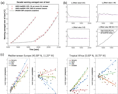
Figure 1.Illustration of the process leading to parameterization of the IMOGEN energy-balance model and the scaled climate patterns (together forming the “pattern-scaling set”), based on the example of the UKMO-HadGEM1 GCM.(a)Emulation of a warming pathway across time. The 1 % to quadrupling atmospheric CO2run was used for calibration of the energy-balance model while the SRES A2 scenario run was used to validate the results.(b)Fitting of the individual EBM parameters, underlining the match presented in(a). Climate sensitivities over landλland oceanλo, as well as the ratio of land to ocean warming rate,ν(pink lines), are derived directly from GCM run data (black curves, 1 % run). The fourth parameter, an ocean effective thermal diffusivity, κ, determines modelled oceanic temperature profile. The κ value is selected based upon comparing calculated values of top-of-profile temperature against global mean SST changes projected by UKMO-HadGEM1 1 % run (shown).(c)Example local fitting of patterns of temperature and precipitation, found as regression coefficients (coloured straight lines) against calculated changes in mean temperature over land from UKMO-HadGEM1. Two representative grid boxes in Mediterranean Europe and tropical Africa are shown. Coloured symbols are decadal mean monthly values from the UKMO-HadGEM1 SRES A2 run, whilst the grey markers represent data from the 20C3M simulation, which were used to normalise to temperature and precipitation change, and are also corresponding to CRU normals (years 1961–1990). Regression pattern fit is forced through [0,0] point, as in diagrams.
Emulating an ensemble of GCMs requires that the re-lationship among anthropogenic climate forcings, global warming and mean warming over land is established for each GCM separately. The EBM employed for this task, described in full in Huntingford and Cox (2000), requires the fitting of five calibration parameters: (1) an ocean effective ther-mal diffusivity,κ(W m−1K−1); (2) a constant ratio of mean land to ocean surface (sea surface temperature, SST) rate of
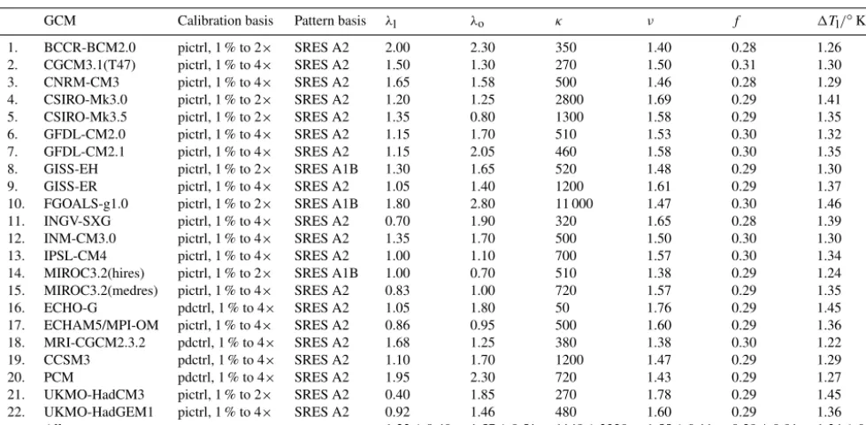
Table 2.Calibration parameters of the simple IMOGEN energy-balance model, for each considered global circulation model. The first column presents which runs (experiments) were used to derive the parameters, listed as follows: (i) an ocean effective thermal diffusivity which determines the uptake of energy,κ(W m−1K−1); (ii) a constant ratio of mean land and ocean surface (sea surface temperature, SST) rate of warming,ν; (iii) climate sensitivity over landλl and (iv) oceanλo(W m−2K−1); and (v)f, which is a land fraction, including Antarctica. The last column presents GCM-specific ratios of warming aver all land per degree of global warming.
GCM Calibration basis Pattern basis λl λo κ ν f 1Tl/◦K
1. BCCR-BCM2.0 pictrl, 1 % to 2× SRES A2 2.00 2.30 350 1.40 0.28 1.26
2. CGCM3.1(T47) pictrl, 1 % to 4× SRES A2 1.50 1.30 270 1.50 0.31 1.30
3. CNRM-CM3 pictrl, 1 % to 4× SRES A2 1.65 1.58 500 1.46 0.28 1.29
4. CSIRO-Mk3.0 pictrl, 1 % to 2× SRES A2 1.20 1.25 2800 1.69 0.29 1.41
5. CSIRO-Mk3.5 pictrl, 1 % to 2× SRES A2 1.35 0.80 1300 1.58 0.29 1.35
6. GFDL-CM2.0 pictrl, 1 % to 4× SRES A2 1.15 1.70 510 1.53 0.30 1.32
7. GFDL-CM2.1 pictrl, 1 % to 4× SRES A2 1.15 2.05 460 1.58 0.30 1.35
8. GISS-EH pictrl, 1 % to 2× SRES A1B 1.30 1.65 520 1.48 0.29 1.30
9. GISS-ER pictrl, 1 % to 4× SRES A2 1.05 1.40 1200 1.61 0.29 1.37
10. FGOALS-g1.0 pictrl, 1 % to 2× SRES A1B 1.80 2.80 11 000 1.47 0.30 1.46
11. INGV-SXG pictrl, 1 % to 4× SRES A2 0.70 1.90 320 1.65 0.28 1.39
12. INM-CM3.0 pictrl, 1 % to 4× SRES A2 1.35 1.70 500 1.50 0.30 1.30
13. IPSL-CM4 pictrl, 1 % to 4× SRES A2 1.00 1.10 700 1.57 0.30 1.34
14. MIROC3.2(hires) pictrl, 1 % to 2× SRES A1B 1.00 0.70 510 1.38 0.29 1.24
15. MIROC3.2(medres) pictrl, 1 % to 4× SRES A2 0.83 1.00 720 1.57 0.29 1.35
16. ECHO-G pdctrl, 1 % to 4× SRES A2 1.05 1.80 50 1.76 0.29 1.45
17. ECHAM5/MPI-OM pictrl, 1 % to 4× SRES A2 0.86 0.95 500 1.60 0.29 1.36
18. MRI-CGCM2.3.2 pdctrl, 1 % to 4× SRES A2 1.68 1.25 380 1.38 0.30 1.22
19. CCSM3 pdctrl, 1 % to 4× SRES A2 1.10 1.70 1200 1.47 0.29 1.29
20. PCM pdctrl, 1 % to 4× SRES A2 1.95 2.30 720 1.43 0.29 1.27
21. UKMO-HadCM3 pictrl, 1 % to 2× SRES A2 0.40 1.85 270 1.78 0.29 1.45
22. UKMO-HadGEM1 pictrl, 1 % to 4× SRES A2 0.92 1.46 480 1.60 0.29 1.36
All 1.23±0.40 1.57±0.51 1148±2220 1.55±0.11 0.29±0.01 1.34±0.06
idealised CO2increase scenario (1pctto2x or 1pctto4x), pre-ceded by a control experiment (Picntrl or Pdcntrl). Subse-quently, functioning of the parameterised EBM was validated by using it predictively against data from one of the available runs corresponding to SRESs (SRES A2 or SRES A1B, Ta-ble 2). Figure 1 illustrates the key components of the process of deriving a pattern-scaling set in the case of the example UKMO-HadGEM1 GCM.
In general, our climate patterns represent absolute changes. However, for precipitation, we make one additional calculation which results in data normalisation. This is to cir-cumvent the problem of particularly large biases in the de-scription of the current precipitation regime by some GCMs (Ines and Hansen, 2006). For each calculated precipitation pattern (1P), this is then multiplied by the ratio of the ob-served precipitation (PCRUXXc) from the CRU TS 2.1 dataset
and the one simulated by the GCM (PGCMXXc) for the
con-trol period. This follows Ines and Hansen (2006) and Malhi et al. (2009):
1P0(g, m, i)=1P (g, m, i)× PCRUXXc(i, mS, gS)
PGCMXXc(i, mS, gS)
. (2)
Furthermore, the adjustment described by Eq. (2) was per-formed for each grid box g, month m and GCM i, after smoothing in time and space (averaging over the grid box and its immediate neighbourhood:gS, and across 3 monthsmS). This smoothing mitigates the minor shifts in seasonality and
spatial positioning of climatic phenomena and reduces sig-nificantly the number of artefacts caused by occasional divi-sion by near zero. The remaining few cases of high and low divergence (i.e.PCRUXXc/PGCMXXc) were capped at 5 and 0.2.
Snow was scaled according to the same scaling factor as for total precipitation. The final pattern set is available in two versions: one with precipitation normalised by Eq. (2) and one without this.
As a last step, in four cases when available GCMs’ data had one or two non-key variables missing (Table 1), the gaps were filled in with across-ensemble means.
3 Results
3.1 Energy-balance parameters
The five key EBM parameters are presented in Table 2. In most cases (17) climate sensitivity over oceans (λo, W m−2K−1) is higher than over land (λ
deter-mines the ability of the ocean to extract heat from the cli-mate system through diffusion. Even after excluding the two most extreme cases, the range remains high: from 270 (HadCM3, CGCM3.1(T47)) to 2800 W m−1K−1 (CSIRO-Mk3.0). The most extreme value of 11 000 W m−1K−1is for the FGOALS-g1.0 GCM, which clearly stands out from the ensemble. (The FGOALS model has been noted as an out-lier in other circumstances – e.g. Atlantic region projections; Perez et al., 2014). This spread reflects the fact that a full un-derstanding of oceanic flows and deeper overturning, which affects mean vertical heat transport, is still required to re-duce model spread. In comparison, the land–ocean temper-ature increase contrast (ν) is a remarkably stable parameter, with a range of 1.40–1.78 across all models.
3.2 Patterns across models, space and seasons
Across models, patterns of particular variables represent con-sistent trends when averaged spatially and across months (Table 3), with a maximum of four exceptions per variable (relative humidity), i.e. cases when the average pattern is of opposite sign than in the majority of GCMs. The pat-terns capture the nature of a new emerging climate regimes, which can be characterised as warmer, wetter (but with less snowfall), cloudier and windier, with decreased relative hu-midity and increased atmospheric pressure. Globally, rela-tive humidity is the variable with the highest uncertainty in the magnitude of change, with standard deviation (SD) of the across-ensemble mean exceeding the mean. In the case of other variables, apart from longwave downward radia-tion and near-surface air temperature (RLDS, TAS, with very small spread), the magnitude of SD is similar (SD of each variable is 62–88 % of the mean).
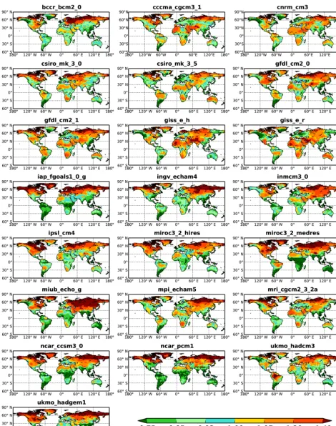
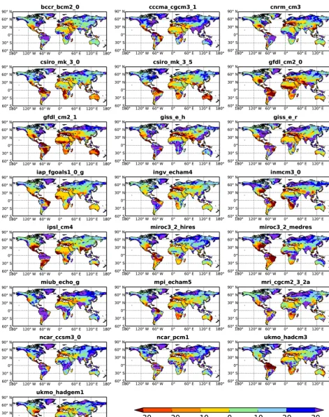
In the case of each GCM, the patterns represent a unique regional and seasonal distribution of change in surface clima-tology in a greenhouse-gas-enriched atmosphere. To present these differences, we focus on two of the strongest drivers of terrestrial ecosystems change (and coincidentally, which also have strong influence on society in general) – that is, adjustments to temperature and precipitation. The annual mean rate of local warming per degree of global warming over land (Fig. 2) in some models is much more evenly dis-tributed geographically (e.g. BCCR-BCM2.0) than in oth-ers (e.g. NCAR-PCM1). However, all of the models exhibit the majority of warming in northern latitudes. The smallest warming occurs in tropical Africa and Asia, while in trop-ical South America the magnitude is much more uncertain. The spatial pattern of warming is either well stratified with latitude (e.g. FGOALS-g1.0 model) or more nuanced (GISS models). The patterns of precipitation change (Fig. 3) are more complex than in the case of temperature. The lack of across-ensemble consistency is particularly apparent in parts of the tropics (e.g. in South America). However, in other ar-eas the signal is very consistent, such as an incrar-ease in dry
conditions in southern Europe or more precipitation in high northern latitudes.
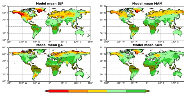
Across-model seasonal averages (Figs. 4 and 5, for tem-perature and precipitation, respectively) reveal a more spa-tially and temporally consistent picture than when consider-ing models individually. These figures show that the major-ity of warming occurs at northern latitudes and during colder seasons. Moreover, there is a strong summer warming trend over mid-western North America, the Mediterranean region, the Middle East and central Asia. The seasonal patterns of precipitation change appear as linked to those of tempera-ture, but are generally more uncertain. Winter warming in the north is accompanied by more precipitation, which contrasts with lower summer warming and reduced rainfall. Changes in tropical rainfall appear as more uncertain. Western and central Africa north of the equator is a zone with particularly high uncertainty regarding summer warming.
Stippling in Fig. 5 provides an additional measure of un-certainty – it indicates when there is agreement in 90 % of the models as to whether precipitation is going to increase or de-crease. This is the case over most of the northern land areas and seasons. However, in many dry areas and seasons where this measure is not robust due to low precipitation levels (and the signal is difficult to detect), the agreement is low. Some areas stand out in this regard: large parts of South America in northern winter and summer, high northern latitudes in the summer and central Asia in autumn. That rainfall changes remain a large uncertainty in climate model projections is noted in the fourth IPCC report (IPCC 2007, Fig. SPM.7) and in the fifth IPCC report (IPCC 2013, Fig. TS.16).
3.3 Performance of linear approximation assumption in “pattern scaling” for individual variables
Table 3.Summary of magnitude, range and robustness of climate change patterns across variables and GCMs. In each table cell, the first value is the mean, followed by the percentage variance explained statistic (PVE, in brackets, underneath). The values in italics are across-ensemble averages used to fill in data gaps (missing variables for some GCMs). In these cases, the PVE statistic was not calculated. Square brackets in the last column denote average PVE (across variables) calculated for these incomplete sets of variables. The penultimate row (All GCMs) contains across-ensemble means of the above statistics, plus associated SDs. The last row presents an additional diagnostic of the pattern-fitting performance – percentage of negative PVE results, which indicate that the one-parameter regression line is a worse fit than the multi-decadal mean.
GCM name TAS HUR UAS+VAS RLDS RSDS PR PRSN PS All
1. BCCR-BCM2.0 1.0463
(83.04) −0.0201 (13.29) 0.0089 (2.66) 5.6754 (76.51) −0.6185 (9.73) 0.0300 (8.16) −0.0025 (13.14) 0.2324 (30.70) (29.65)
2. CGCM3.1(T47) 1.0561 (85.79) 0.0974 (19.80) 0.0197 (8.30) 6.0605 (87.28) −0.4722 (18.82) 0.0448 (18.71) −0.0015 (16.66) 0.0730 (21.33) (34.59)
3. CNRM-CM3 1.0371
(86.64) −0.0111 (24.84) 0.0098 (8.73) 5.7499 (81.41) −0.4978 (19.65) 0.0255 (17.05) 0.0000 (17.35) 0.1838 (38.48) (36.77)
4. CSIRO-Mk3.0 1.0740
(82.73) −0.2354 (13.99) 0.0108 (–) 5.9023 (84.39) −0.6072 (24.46) 0.0165 (9.38) −0.0032 (25.70) 0.0947 (–) [40.11]
5. CSIRO-Mk3.5 1.0270
(87.73) −0.2214 (17.04) 0.0059 (6.93) 6.2917 (87.92) −0.3596 (25.23) 0.0044 (12.42) −0.0035 (17.22) 0.0138 (21.94) (34.56)
6. GFDL-CM2.0 1.0731
(83.58) −0.2653 (14.77) 0.0071 (8.25) 6.0471 (83.69) −1.8451 (34.58) 0.0042 (16.89) −0.0041 (21.49) 0.0657 (24.35) (35.95)
7. GFDL-CM2.1 1.0794
(79.71) −0.2310 (17.35) 0.0113 (9.59) 6.2023 (82.62) −1.7225 (33.21) −0.0017 (17.93) −0.0067 (18.66) 0.2057 (29.21) (36.03)
8. GISS-EH 1.0543
(75.71) 0.0080 (10.48) 0.0103 (4.25) 6.6734 (77.09) −1.4802 (1.95) 0.0415 (11.28) −0.0016 (8.04) 0.0264 (12.18) (25.12)
9. GISS-ER 1.0365
(80.07) −0.1572 (17.25) 0.0099 (7.08) 6.1883 (–) −0.9399 (11.05) 0.0384 (14.76) −0.0018 (10.16) 0.0251 (18.31) [22.67]
10. FGOALS-g1.0 1.1180 (83.05) −0.0980 (4.11) −0.0031 (1.36) 6.3137 (82.71) −0.9748 (9.67) 0.0205 (6.70) −0.0010 (15.52) 0.0836 (13.62) (27.09)
11. INGV-SXG 1.0863
(88.01) −0.0209 (22.96) 0.0128 (5.20) 6.2418 (–) −0.7667 (–) 0.0184 (10.68) −0.0067 (19.10) 0.0217 (18.58) (35.98)
12. INM-CM3.0 1.0604
(83.51) −0.0391 (15.44) 0.0130 (4.88) 5.7124 (78.17) −0.2908 (23.54) 0.0200 (14.32) −0.0071 (12.97) 0.0124 (16.43) (31.16)
13. IPSL-CM4 1.1043
(90.18) −0.6717 (27.46) 0.0059 (9.92) 6.1517 (85.26) 0.0932 (27.85) 0.0166 (15.72) −0.0089 (23.73) 0.1216 (21.31) (37.68)
14. MIROC3.2(hires) 1.0801 (94.19) −0.1528 (16.89) 0.0031 (8.45) 6.2088 (92.28) −1.0731 (36.21) 0.0271 (20.90) −0.0052 (25.45) 0.2352 (37.87) (41.53)
15. MIROC3.2(medres) 1.1281 (91.16) −0.2819 (15.56) 0.0062 (9.38) 6.4687 (88.97) −1.7130 (38.30) 0.0272 (22.37) −0.0032 (23.53) 0.1417 (30.26) (39.94)
16. ECHO-G 1.1383
(88.41) −0.1256 (–) 0.0165 (9.54) 6.5682 (86.84) −1.4149 (20.41) 0.0574 (18.77) −0.0046 (21.54) −0.0648 (19.65) [37.88]
17. ECHAM5/MPI-OM 1.0726 (89.81) −0.2200 (18.66) 0.0173 (8.35) 6.1048 (89.35) −0.3009 (18.78) 0.0294 (14.08) −0.0052 (17.45) 0.0714 (22.61) (34.89)
18. MRI-CGCM2.3.2 1.0641 (84.62) 0.6378 (13.21) −0.0048 (3.25) 6.5956 (82.92) −1.2903 (10.43) 0.0387 (7.60) −0.0063 (–) 0.0979 (17.37) [31.34]
19. CCSM3 1.1182
(87.92) −0.0307 (15.09) 0.0091 (6.75) 6.8102 (89.67) −1.2080 (24.48) 0.0477 (21.47) −0.0071 (20.45) 0.1629 (25.02) (36.36)
20. PCM 1.1059
(78.64) 0.0704 (9.65) 0.0346 (1.13) 6.2678 (75.20) −0.9678 (8.34) 0.0573 (12.52) 0.0009 (13.56) 0.1509 (17.32) (27.04)
21. UKMO-HadCM3 1.0572 (86.57) −0.7051 (29.40) 0.0137 (9.85) 5.6891 (84.81) 0.2089 (27.15) 0.0096 (16.36) −0.0036 (15.88) −0.0542 (23.05) (36.63)
22. UKMO-HadGEM1 1.1222 (88.60) −0.0900 (18.05) 0.0190 (15.49) 6.2180 (89.33) −1.9194 (37.04) 0.0076 (21.45) −0.0039 (22.27) 0.1814 (32.21) (40.55)
All GCMs 1.079±
0.032 (85.44±
4.37)
−0.1256±
0.2579 (16.92±
5.71)
0.0108±
0.0080 (7.11±
3.32)
6.188±
0.400 (84.74±
4.97)
−0.9164±
0.6000 (23.29±
10.23)
0.0264±
0.0165 (14.98±
4.61)
−0.0040±
0.0025 (17.96±
4.67)
0.095±
0.084 (23.33±
6.99)
(34.25±
5.21)
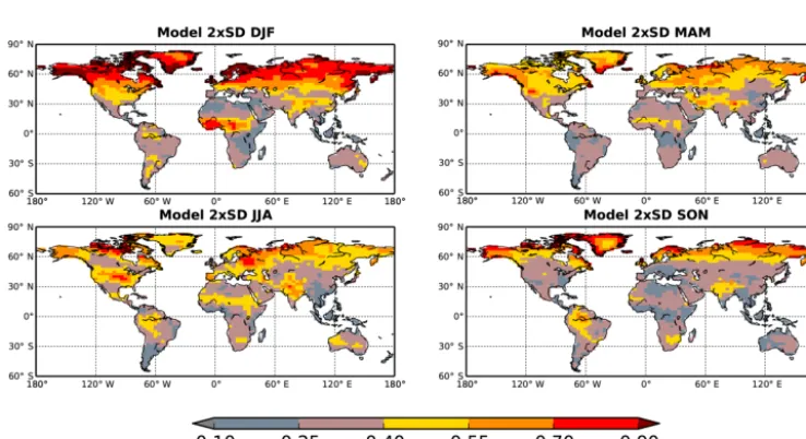
Figure 4.Seasonal means and variation (2×SD) of the monthly patterns of local temperature change per degree warming over all land (K K−1), across 22 GCMs. DJF is December, January and February; MAM is March, April and May; JJA is June, July and August; and SON is September, October and November.
Overall (i.e. when per-variable results are averaged, with-out considering co-variance), climate patterns explain one-third of regional climate change (PVE 34.25±5.21); how-ever, the signal in some models exhibits much more linear-ity (e.g. MIROC3.2(hires): 41.53) than in others (GISS_ER: 22.67). These estimates exclude cases where the PVE statis-tic could not be calculated due to either a lack of data (2.8 %, Table 1), or null (e.g. shortwave radiation during polar night) or extremely low values (e.g. precipitation in the dry season), accounting for 6.7 % of cases.
In terms of spatial distribution of robustness of the two key variables, temperature and precipitation (Fig. 6), it is
Figure 5.Seasonal means and variation (2×SD) in the monthly patterns of local precipitation change per degree warming over all land (mm yr−1K−1), across 22 GCMs. In regions marked with stippling dots, more than 90 % of the models agree in the sign of the change, whilst hatching is where less than 66 % of the models agree in sign. DJF is December, January and February; MAM is March, April and May; JJA is June, July and August; and SON is September, October and November.
4 Applications
The pattern-scaling concept was originally designed as a tool for scientists to inform policymakers, enabling investigation of expected changes in surface climatology for a broader range of scenarios of atmospheric greenhouse gas concentra-tions than are available in archived GCM runs. The technique has been studied in depth, and one study recently concluded that “Overall, the well-established validity of the technique in approximating the forced signal of change under increasing
Figure 6. Seasonal percentage of variance explained of the monthly patterns of local temperature and precipitation change per degree warming, across 22 GCMs. DJF is December, January and February; MAM is March, April and May; JJA is June, July and August; and SON is September, October and November.
process responses in a changing climate. This is often for similar forcing scenarios to those that GCMs have been op-erated for, but with the full climate models not yet running with the new land surface descriptions modelled in IMO-GEN. Particular examples include quantification of wetland methane feedbacks (Gedney et al., 2004), the impacts of changes in diffuse radiation to the land carbon sink (Mercado et al., 2009), the effects of tropospheric ozone on plant pro-ductivity (Sitch et al., 2007), the significance of energy crop planting on future atmospheric CO2concentration (Hughes et al., 2010), and how alternative mixtures of changes in at-mospheric composition, even corresponding to identical
ra-diative forcing changes, can have very contrasting impacts on land surface carbon stocks (Huntingford et al., 2011), and permafrost climate–carbon cycle feedbacks in a warm-ing world (Burke et al., 2017).
to (i) some limited uncertainty via prescribed bounds in the parameterisations of the atmospheric component of UKMO-HadCM3 (related to UKMO-HadCM3LC), (ii) description of canopy radiation interception – “big leaf” vs. “multilayer” (Mercado et al., 2007) – and (iii) representation of vegetation dynam-ics using an area-based model and an individual-based model (Moorcroft et al., 2001). All simulations show a fairly robust risk of dieback. More recently, a set of the climate patterns described in this paper were used to re-analyse the potential for tropical rainforest dieback. Zelazowski et al. (2011) com-bined the patterns and global contemporary climatology to produce high-resolution maps of the future extent of humid tropical forests, while Huntingford et al. (2013c) forced the IMOGEN framework with the full set of patterns. Both stud-ies found that climate models other than UKMO-HadCM3 are less likely to project such rainforest losses, which reflects the particularly strong climatic signal for the Amazon region temperature and precipitation changes for UKMO-HadCM3, as noted in Figs. 2 and 3.
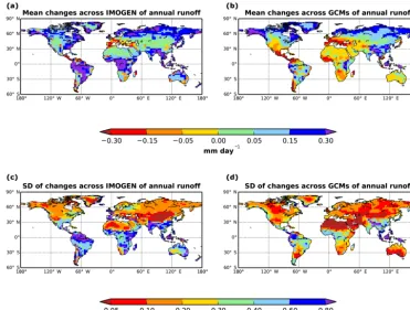
In order to exemplify the ability of IMOGEN to project changes to impacts, we report results of the mean annual total runoff (Rtot, mm day−1) simulation based on the SRES A1B emissions forcing scenario (Fig. 7), and we compare them directly to GCM estimates of change in the same quantity. Hence, this is comparing the IMOGEN simulations that em-ulate multiple GCMs but with a single land surface model (JULES), vs. runoff values directly from the GCMs. The lat-ter therefore contains allat-ternative estimates of climate change, as well as the responses of different land surface models. During a modelled pre-industrial control “spin-up” period and a modelled period centred on year 2090, total runoff values are recorded for each GCM (both emulated in IMO-GEN, and taken directly from GCMs). Then, in each case, the change is calculated. In Fig. 7a–b, the mean of these changes is shown, whilst Fig. 7c–d show the SDs of these change values. Although there are similarities between the left- and right-hand panels (over northern latitudes, in par-ticular), there are important differences too, and notably the drying signal in GCM output for Africa and Australia is not reflected in the IMOGEN framework. For SDs, in some lo-cations there is higher variability for IMOGEN than for the GCMs themselves; however, this pertains mainly to the re-gions where IMOGEN predicts higher runoff. The latter may be surprising, considering that GCMs directly introduce an-other level of uncertainty, i.e. inter-land surface model dif-ferences. Our finding is suggestive that JULES has a par-ticularly sensitive response of runoff to imposed climatic changes. Runoff provides a challenge for comparison, as it is frequently a relatively small number between two larger fluxes of precipitation and evapotranspiration (transpiration, plus soil evaporation and interception losses) and so is sen-sitive to change in those fluxes. Any direct comparison also needs to account for IMOGEN being initialised with a clima-tology based on the CRU dataset and temporal disaggrega-tion to sub-daily drivers of JULES having not been calibrated
against any particular GCM. Nevertheless, to be a useful tool for impacts assessment, then IMOGEN must capture the gen-eral features of GCM projections of quantities such as runoff when operated for similar emissions scenarios.
Looking ahead to further model development, one pos-sibility is for different GCMs to directly pattern-scale im-pact variables of interest, such as runoff, against global land temperature change. This could be beneficial for two rea-sons. First, it would remove the current IMOGEN mismatch of many GCMs emulated based on their climate projections only, while the emulating system is coupled to just one land surface model. Instead, a more accurate representation would be gained from the spread of runoff uncertainty. Second, it would make model calculations computationally very fast, as full operation of the JULES system would not be required. Such an approach would be applicable when using IMOGEN to estimate changes for different future greenhouse gas con-centrations, rather than land surface modelling development. A further possibility is to connect the meteorological pattern-scaling structure to alternative land surface models. The anal-ysis of Sitch et al. (2008) used the IMOGEN system to diag-nose uncertainty in representation of future plant biogeogra-phy and climate–carbon cycle feedbacks using five dynami-cal global vegetation models (DGVMs), but then combined them with only a single set of climate model patterns based on UKMO-HadCM3. This could be revisited. If each DGVM modelling centre could operate their latest DGVM configu-ration, across the range of emulated GCMs, then this would give a fuller estimate of the balance between implications of uncertainty in climate and uncertainty in terrestrial ecosys-tem response and its feedbacks on the global carbon cycle. A full set of calculations would entail 5 times 22 simulations, for a single future atmospheric greenhouse gas concentration pathway or emissions pathway. This capability could be of interest to research programs designed to compare different estimates of impacts under climate change (e.g. the Inter-Sectoral Impact Model Intercomparison Project, ISIMIP).
Figure 7.Comparison of IMOGEN and GCM estimates of annual mean runoff changes. This is for 20 years centred on 2090 minus 20 years centred on 1900, and for emissions scenario SRES A1B.(a)shows the mean changes in runoff across GCMs emulated in the IMOGEN system, all forcing the JULES land surface model.(b)shows the mean changes in runoff as taken directly from the GCMs themselves.(c), at each grid box, presents the SD of changes in runoff for IMOGEN, again across GCMs emulated.(d)shows SD of changes in runoff taken directly from the GCMs.
JULES (Zaehle et al., 2010). Furthermore, it is desirable to test the effects of adding height competition into the vege-tation dynamics module of JULES, in order to add ecolog-ical succession modelling (Smith et al., 2001; Moorecroft et al., 2001), as well as assess the impacts of improved repre-sentation of stomatal conductance (Medlyn et al., 2011; Kala et al., 2015) and plant hydraulics (Sperry et al., 2016) on sim-ulated land carbon and water cycles couplings to climate. The latter could extend as far as testing any hormonal signalling in the hydraulic linkages between soil moisture and stomata response, an effect well known by the physiological commu-nity but heretofore never tested in a full large-scale gridded land surface model (Huntingford et al., 2015). Finally, the impacts of introducing a better representation of plant func-tional types and plant trait variation across space and time (Verheijen et al., 2015) on simulated land carbon could also be considered.
5 Discussion
In this paper we present a pattern-scaling set, consisting of spatially explicit climate change patterns and EBM calibra-tion parameters, which together represent 22 GCMs of the
WCRP CMIP3 database (Meehl et al., 2007a). This dataset extends the use of the IMOGEN climate-impact assessment tool to scan across uncertainty in climate models. Despite re-lying on a set of simple assumptions, the tool can capture a significant part of the predicted changes in surface clima-tology. Terrestrial ecosystem response studies have used this modelling framework to gain new insights into how the land surface component of the Earth system functions. A new ver-sion of the pattern-scaling set, based on the CMIP5 dataset, will build on those available here.
two stabilised limits (Huntingford et al., 2017) to force GEN in this configuration. A further advantage of the IMO-GEN system is that the projected anomalies of meteorologi-cal change are generally added to known gridded climatolo-gies, rather than to any GCM-based baseline estimates. One such dataset is the routinely updated Climate Research Unit climatology (Harris et al., 2014). A typical estimate of pre-industrial conditions may be regarded as the mean climatol-ogy of a period such as 1960–1989, a time when weather sta-tions had become much more available worldwide to guide the dataset construction. Although this will fail to capture warming effects between pre-industrial times and that period, such offsets may be much smaller than the biases removed by not using GCMs to estimate a baseline climatology to which IMOGEN anomalies are added. This does, though, assume such GCM bias removal is valid for the entirety of any tran-sient simulation. Recent analyses appeal for more process in-formation to be accounted for when attempting bias correc-tion (Maraun et al., 2017).
An important aspect of the presented work is the com-prehensive study of the pattern’s robustness, i.e. their ability to capture variability of climate simulated by GCMs. That across all variables considered, one-third of decadal variabil-ity in monthly averages is captured, suggests that it is a tech-nique with a significant potential. This is especially impor-tant since it allows a large reduction in input data and com-putation requirements compared to full GCMs. Overall, the presented patterns are in good agreement with the results pre-sented in the Fourth Assessment Report of the Intergovern-mental Panel on Climate Change (e.g. for precipitation Sup-plement, Fig. S1 in the Supplement and Fig. 10.9 in Meehl et al., 2007b). This applies to both the multi-model mean changes in surface climate, as well as the degree of agree-ment between the models (stippling in Fig. 5 and Fig. S2).
However, the ability of climate patterns to capture the course of changes varies significantly between the mod-elled climate variables. In contrast to temperature change (85.44±4.37 % of variability explained by climate patterns), change in precipitation is usually more difficult to capture in this linear methodology. Overall 85 % of precipitation vari-ability remains unexplained, although it should be noted that in some regions seasonal precipitation patterns explain up to 75 % of variability (generally at high northern latitudes). The relatively weak explanatory power of the precipitation pat-terns can be partly explained by poor trend estimation over dry zones. In these areas, the mean change over decades gives low PVE values, as any change in very small current abso-lute precipitation can result in high relative deviations from pre-industrial levels. In such circumstances, precipitation is very much dominated by inter-annual fluctuations.
In addition to uncertainty linked to methods and assump-tions (such as linearity), there is some uncertainty linked di-rectly to driving and calibrating input data. The decision to use 20C3M and SRESs to derive patterns, as well as the ide-alised scenario of 1 % annual CO2 increase to calibrate the
EBM model, reflects a compromise between the accuracy of patterns and forcings. It could be argued that both the patterns and the EBM parameters should be derived from the same set of GCM runs. However, since the SRES runs are on average longer (12 decades, with part of the 20C3M run), they are therefore a better source for linear fitting of the spatial pat-terns (Mitchel, 2003). However, the idealised CO2increase scenarios are a better basis for energy-balance model calibra-tion as the definicalibra-tion of SRES forcings varies between mod-elling groups (they often encompass atmospheric aerosols) and these forcings are less well documented.
Although placing climate data on a common grid brings strong benefits to the IMOGEN tool, there is also a compro-mise. For the re-gridding method combined with land map-ping (see Supplement), the calculated regional patterns rep-resent areas that comprise fully of land, while in much of original GCM data, grid boxes represent a mix of land and ocean. The total land fraction in the presented spatial patterns is slightly increased due to this (see Fig. S2). This increases the average grid-box warming, due to diminished represen-tation of the oceanic heat uptake. As a result, the fitting pro-cedure yields regional warming patterns (column “TAS” in Table 3) which, when area-weighted, overall return a value slightly larger than 1.0 K K−1. However, this effect has no impact on the global energy budget in the IMOGEN frame-work, which is resolved independently with EBM.
There are a number of potential methodological enhance-ments that can be implemented in the next IMOGEN version and beyond just fitting to the CMIP5 (Taylor et al., 2012) or CMIP6 (Eyring et al., 2016) datasets. For example, so far, the natural variability around the trend in IMOGEN is simulated through a daily “weather generator” component with invariant properties, and with no representation of inter-annual variability. However, variability might also change in a warming world, and at a range of timescales from sub-daily through to major alteration on inter-annual timescales (e.g. Huntingford et al., 2013a). This suggests that in fu-ture research, at least for some variables, additional patterns might be added that capture such variability changes and in-clude any inter-annual variability and adjustment for differ-ent warming levels.
feed-backs are not constant in time, and different components of the climate system respond on different timescales (Chad-wick and Good, 2013). This implies that, should IMOGEN be used to test significantly different land surface parameter-isations, projected local and regional meteorological changes might no longer be compatible.
Nevertheless, as long as IMOGEN is used with aware-ness of its limitations, then it offers a simple, available and computationally fast way to emulate GCMs. This can be op-erated to estimate surface meteorological changes for dif-ferent future atmospheric greenhouse pathways. It can also be operated to undertake intermediate analysis with new land surface process descriptions, before their operation in full-complexity GCMs. This paper takes the further step of adding to its capability the scanning across of a large set of GCMs that it now emulates. Ultimately, the CMIP5 ensem-ble, which formed the basis of the recent fifth IPCC report (IPCC, 2013) using diagnostics available at that time, has much potential to improve the performance of the described pattern-scaling framework. Aside from the fact that the mod-els themselves have improved, more scenarios are available, allowing better assessment of forcings other than CO2. With preparations now starting for the sixth IPCC report, and new simulations being made for that, it is timely to consolidate and calibrate a new set of patterns for the CMIP5 family of GCMs, building on the analysis presented in this paper.
Code and data availability. The IMOGEN version 2.0 patterns and EBM parameters, along with documentation, are available for full download (under “IMOGEN”) from the UK Environmental Infor-mation Data Centre (EIDC; http://eidc.ceh.ac.uk). The IMOGEN framework (Huntingford et al., 2010) has become a component of the JULES land surface initiative (Best et al., 2011; Clark et al., 2011), and it is available via that route (http://jules.jchmr.org). For the most up-to-date IMOGEN code, please contact the correspond-ing author.
Supplement. The supplement related to this article is available online at: https://doi.org/10.5194/gmd-11-541-2018-supplement.
Author contributions. PZ performed the fitting of the patterns and EBM parameters against the CMIP3 database. CH developed the overall IMOGEN model framework. LMM advised on impact ap-plications and NS aided with placing of the analysis in context in terms of other GCM emulation systems. All authors contributed to-wards writing the paper.
Competing interests. The authors declare that they have no conflict of interest.
Acknowledgements. We acknowledge the modelling groups, the Program for Climate Model Diagnosis and Intercomparison, and the World Climate Research Programme (WCRP) Working Group on Coupled Modelling for their roles in making available the WCRP Coupled Model Intercomparison Project 3 multi-model dataset. This work was financially supported by the Natural Environment Research Council (UK), pilot project Environmental Virtual Observatory (NE/I002200/1), and by the National Science Centre (Poland), grant SONATA 2014/13/D/ST10/00022. Chris Huntingford was also supported by CEH National Capability funds. We thank Seiji Yukimoto of the Climate Research Department, Meteorological Research Institute, Japan, for assistance in process-ing MRI-CGCM2.3.2 data.
Edited by: Wilco Hazeleger
Reviewed by: two anonymous referees
References
Atkin, O. K., Bloomfield, K. J., Reich, P. B., Tjoelker, M. G., Asner, G. P., Bonal, D., Bonisch, G., Bradford, M. G., Cernusak, L. A., Cosio, E. G., Creek, D., Crous, K. Y., Domingues, T. F., Dukes, J. S., Egerton, J. J. G., Evans, J. R., Farquhar, G. D., Fyllas, N. M., Gauthier, P. P. G., Gloor, E., Gi-meno, T. E., Griffin, K. L., Guerrieri, R., Heskel, M. A., Hunt-ingford, C., Ishida, F. Y., Kattge, J., Lambers, H., Liddell, M. J., Lloyd, J., Lusk, C. H., Martin, R. E., Maksimov, A. P., Maxi-mov, T. C., Malhi, Y., Medlyn, B. E., Meir, P., Mercado, L. M., Mirotchnick, N., Ng, D., Niinemets, U., O’Sullivan, O. S., Phillips, O. L., Poorter, L., Poot, P., Prentice, I. C., Sali-nas, N., Rowland, L. M., Ryan, M. G., Sitch, S., Slot, M., Smith, N. G., Turnbull, M. H., VanderWel, M. C., Valladares, F., Veneklaas, E. J., Weerasinghe, L. K., Wirth, C., Wright, I. J., Wythers, K. R., Xiang, J., Xiang, S., and Zaragoza-Castells, J.: Global variability in leaf respiration in relation to climate, plant functional types and leaf traits, New Phytol., 206, 614–636, https://doi.org/10.1111/nph.13253, 2015.
Best, M. J., Pryor, M., Clark, D. B., Rooney, G. G., Essery, R. L. H., Ménard, C. B., Edwards, J. M., Hendry, M. A., Porson, A., Gedney, N., Mercado, L. M., Sitch, S., Blyth, E., Boucher, O., Cox, P. M., Grimmond, C. S. B., and Harding, R. J.: The Joint UK Land Environment Simulator (JULES), model description – Part 1: Energy and water fluxes, Geosci. Model Dev., 4, 677–699, https://doi.org/10.5194/gmd-4-677-2011, 2011.
Booth, B. B. B., Jones, C. D., Collins, M., Totterdell, I. J., Cox, P. M., Sitch, S., Huntingford, C., Betts, R. A., Harris, G. R., and Lloyd, J.: High sensitivity of future global warming to land carbon cycle processes, Environ. Res. Lett., 7, 024002, https://doi.org/10.1088/1748-9326/7/2/024002, 2012.
Burke, E. J., Ekici, A., Huang, Y., Chadburn, S. E., Huntingford, C., Ciais, P., Friedlingstein, P., Peng, S. S., and Krinner, G.: Quanti-fying uncertainties of permafrost carbon-climate feedbacks, En-viron. Res. Lett., 14, 3051–3066, https://doi.org/10.5194/bg-14-3051-2017, 2017.
Clark, D. B., Mercado, L. M., Sitch, S., Jones, C. D., Gedney, N., Best, M. J., Pryor, M., Rooney, G. G., Essery, R. L. H., Blyth, E., Boucher, O., Harding, R. J., Huntingford, C., and Cox, P. M.: The Joint UK Land Environment Simulator (JULES), model description – Part 2: Carbon fluxes and vegetation dynamics, Geosci. Model Dev., 4, 701–722, https://doi.org/10.5194/gmd-4-701-2011, 2011.
Cox, P. M., Betts, R. A., Jones, C. D., Spall, S. A., and Totter-dell, I. J.: Acceleration of global warming due to carbon-cycle feedbacks in a coupled climate model, Nature, 408, 184–187, https://doi.org/10.1038/35041539, 2000.
Cox, P. M., Betts, R. A., Collins, M., Harris, P. P., Huntingford, C., and Jones, C. D.: Amazonian forest dieback under climate-carbon cycle projections for the 21st century, Theor. Appl. Cli-matol., 78, 137–156, https://doi.org/10.1007/s00704-004-0049-4, 2004.
Eyring, V., Bony, S., Meehl, G. A., Senior, C. A., Stevens, B., Stouffer, R. J., and Taylor, K. E.: Overview of the Coupled Model Intercomparison Project Phase 6 (CMIP6) experimen-tal design and organization, Geosci. Model Dev., 9, 1937–1958, https://doi.org/10.5194/gmd-9-1937-2016, 2016.
Frieler, K., Meinshausen, M., Mengel, M., Braun, N., and Hare, W.: A scaling approach to probabilistic assessment of regional climate change, J. Climate, 25, 3117–3144, https://doi.org/10.1175/JCLI-D-11-00199.1, 2012.
Gedney, N., Cox, P. M., and Huntingford, C.: Climate feed-back from wetland methane emissions, Geophys. Res. Lett., 31, L20503, https://doi.org/10.1029/2004GL020919, 2004. Good, P., Gregory, J. M., and Lowe, J. A.: A
step-response simple climate model to reconstruct and interpret AOGCM projections, Geophys. Res. Lett., 38, L01703, https://doi.org/10.1029/2010GL045208, 2011.
Harris, I., Jones, P. D., Osborn, T. J., and Lister, D. H.: Up-dated high-resolution grids of monthly climatic observations – the CRU TS3.10 Dataset, Int. J. Climatol., 34, 623–642, https://doi.org/10.1002/joc.3711, 2014.
Hughes, J. K., Lloyd, A. J., Huntingford, C., Finch, J. W., and Harding, R. J.: The impact of extensive planting of Miscant-hus as an energy crop on future CO2 atmospheric concentra-tions, GCB Bioenergy, 2, 79–88, https://doi.org/10.1111/j.1757-1707.2010.01042.x, 2010.
Huntingford, C. and Cox, P. M.: An analogue model to derive additional climate change scenarios from ex-isting GCM simulations, Clim. Dynam., 16, 575–586, https://doi.org/10.1007/s003820000067, 2000.
Huntingford, C., Harris, P. P., Gedney, N., Cox, P. M., Betts, R. A., Marengo, J. A., and Gash, J. H. C.: Using a GCM analogue model to investigate the potential for Ama-zonian forest dieback, Theor. Appl. Climatol., 78, 177–185, https://doi.org/10.1007/s00704-004-0051-x, 2004.
Huntingford, C., Fisher, R. A., Mercado, L., Booth, B. B. B., Sitch, S., Harris, P. P., Cox, P. M., Jones, C. D., Betts, R. A., and Malhi, Y: Towards quantifying uncertainty in predictions of Amazon “dieback”, Philos. T. Roy. Soc. B., 363, 1857–1864, https://doi.org/10.1098/rstb.2007.0028, 2008.
Huntingford, C., Booth, B. B. B., Sitch, S., Gedney, N., Lowe, J. A., Liddicoat, S. K., Mercado, L. M., Best, M. J., Wee-don, G. P., Fisher, R. A., Lomas, M. R., Good, P., Zelazowski, P., Everitt, A. C., Spessa, A. C., and Jones, C. D.: IMOGEN:
an intermediate complexity model to evaluate terrestrial im-pacts of a changing climate, Geosci. Model Dev., 3, 679–687, https://doi.org/10.5194/gmd-3-679-2010, 2010.
Huntingford, C., Cox, P. M., Mercado, L. M., Sitch, S., Bel-louin, N., Boucher, O., and Gedney, N.: Highly contrast-ing effects of different climate forccontrast-ing agents on terrestrial ecosystem services, Philos. T. R. Soc. A, 369, 2026–2037, https://doi.org/10.1098/rsta.2010.0314, 2011.
Huntingford, C., Jones, P. D., Livina, V. N., Lenton, T. M., and Cox, P. M.: No increase in global temperature variabil-ity despite changing regional patterns, Nature, 500, 327–330, https://doi.org/10.1038/nature12310, 2013a.
Huntingford, C., Mercado, L., and Post, E.: Earth science the timing of climate change, Nature, 502, 174–175, 2013b.
Huntingford, C., Zelazowski, P., Galbraith, D., Mercado, L. M., Sitch, S., Fisher, R., Lomas, M., Walker, A. P., Jones, C. D., Booth, B. B. B., Malhi, Y., Hemming, D., Kay, G., Good, P., Lewis, S. L., Phillips, O. L., Atkin, O. K., Lloyd, J., Gloor, E., Zaragoza-Castells, J., Meir, P., Betts, R., Harris, P. P., Nobre, C., Marengo, J., and Cox, P. M.: Simulated resilience of tropical rainforests to CO2-induced climate change, Nat. Geosci., 6, 268– 273, https://doi.org/10.1038/NGEO1741, 2013c.
Huntingford, C., Smith, D. M., Davies, W. J., Falk, R., Sitch, S., and Mercado, L. M.: Combining the ABA and net photosynthesis-based model equations of stomatal conductance, Ecol. Model., 300, 81–88, https://doi.org/10.1016/j.ecolmodel.2015.01.005, 2015.
Huntingford, C., Yang, H., Harper, A., Cox, P. M., Gedney, N., Burke, E. J., Lowe, J. A., Hayman, G., Collins, W. J., Smith, S. M., and Comyn-Platt, E.: Flexible parameter-sparse global temperature time profiles that stabilise at 1.5 and 2.0◦C, Earth Syst. Dynam., 8, 617–626, https://doi.org/10.5194/esd-8-617-2017, 2017.
Ines, A. V. M. and Hansen, J. W.: Bias correction of daily GCM rainfall for crop simulation studies, Agr. Forest Meteorol., 138, 44–53, https://doi.org/10.1016/j.agrformet.2006.03.009, 2006. IPCC: Climate Change 2007: The Physical Science Basis,
Con-tribution of Working Group I to the Fourth Assessment Report of the Intergovernmental Panel on Climate Change, edited by: Solomon, S., Qin, D., Manning, M., Chen, Z., Marquis, M., Av-eryt, K. B., Tignor, M., and Miller, H. L., Cambridge University Press, Cambridge, UK and New York, NY, USA, 996 p., 2007. IPCC: Climate Change 2013: The Physical Science Basis,
Con-tribution of Working Group I to the Fifth Assessment Report of the Intergovernmental Panel on Climate Change, edited by: Stocker, T. F., Qin, D., Plattner, G.-K., Tignor, M., Allen, S. K., Boschung, J., Nauels, A., Xia, Y., Bex, V., and Midgley, P. M., Cambridge University Press, Cambridge, UK and New York, NY, USA, 1535 pp., 2013.
James, R., Washington, R., Schleussner, C.-F., Rogelj, J., and Conway, D.: Characterizing half-a-degree difference: a re-view of methods for identifying regional climate responses to global warming targets, WIRES Clim. Change, 8, e457, https://doi.org/10.1002/wcc.457, 2017.
Kala, J., De Kauwe, M. G., Pitman, A. J., Lorenz, R., Medlyn, B. E., Wang, Y.-P., Lin, Y.-S., and Abramowitz, G.: Implementa-tion of an optimal stomatal conductance scheme in the Australian Community Climate Earth Systems Simulator (ACCESS1.3b), Geosci. Model Dev., 8, 3877–3889, https://doi.org/10.5194/gmd-8-3877-2015, 2015.
Malhi, Y., Aragao, L. E. O. C., Galbraith, D., Huntingford, C., Fisher, R., Zelazowski, P., Sitch, S., McSweeney, C., and Meir, P.: Exploring the likelihood and mechanism of a climate-change induced dieback of the Amazon rainforest, P. Natl. Acad. Sci. USA, 106, 20610–20615, https://doi.org/10.1073/pnas.0804619106, 2009.
Maraun, D., Shepherd, T. G., Widmann, M., Zappa, G., Walton, D., Gutiérrez, J. M., Hagemann, S., Richter, I., Soares, P. M. M., Hall, A., and Mearns, L. O.: Towards process-informed bias cor-rection of climate change simulations, Nat. Clim. Change, 7, 764–773, https://doi.org/10.1038/nclimate3418, 2017.
Medlyn, B. E., Duursma, R. A., Eamus, D., Ellsworth, D. S., Pren-tice, I. C., Barton, C. V. M., Crous, K. Y., de Angelis, P., Free-man, M., and Wingate, L.: Reconciling the optimal and em-pirical approaches to modelling stomatal conductance, Glob. Change Biol., 17, 2134–2144, https://doi.org/10.1111/j.1365-2486.2010.02375.x, 2011.
Meehl, G. A., Covey, C., Delworth, T., Latif, M., McAvaney, B., Mitchell, J. F. B., Stouffer, R. J., and Taylor, K. E.: The WCRP CMIP3 multimodel dataset – a new era in climate change research, B. Am. Meteorol. Soc., 88, 1383–1394, https://doi.org/10.1175/BAMS-88-9-1383, 2007a.
Meehl, G. A., Stocker, T. F., Collins, W. D., Friedlingstein, P., Gaye, A. T., Gregory, J. M., Kitoh, A., Knutti, R., Murphy, J. M., Noda, A., Raper, S. C. B., Watterson, I. G., Weaver, A. J., and Zhao, Z.-C.: Global Climate Projections, in: Climate Change 2007: The Physical Science Basis, Contribution of Working Group I to the Fourth Assessment Report of the Intergovernmen-tal Panel on Climate Change, edited by: Solomon, S., Qin, D., Manning, M., Chen, Z., Marquis, M., Averyt, K. B., Tignor, M. and Miller, H. L., Cambridge University Press, Cambridge, UK and New York, NY, USA, 996 p., 2007b.
Mercado, L. M., Huntingford, C., Gash, J. H. C., Cox, P. M., and Jogireddy, V.: Improving the representation of radiation intercep-tion and photosynthesis for climate model applicaintercep-tions, Tellus B, 59, 553–565, https://doi.org/10.1111/j.1600-0889.2007.00256.x, 2007.
Mercado, L. M., Bellouin, N., Sitch, S., Boucher, O., Hunting-ford, C., Wild, M., and Cox, P. M.: Impact of changes in diffuse radiation on the global land carbon sink, Nature, 458, 1014-U87, https://doi.org/10.1038/nature07949, 2009.
Mercado, L. M., Patino, S., Domingues, T. F., Fyllas, N. M., Weedon, G. P., Sitch, S., Quesada, C. A., Phillips, O. L., Aragao, L. E. O. C., Malhi, Y., Dolman, A. J., Restrepo-Coupe, N., Saleska, S. R., Baker, T. R., Almeida, S., Higuchi, N., and Lloyd, J.: Variations in Amazon forest productivity cor-related with foliar nutrients and modelled rates of photosyn-thetic carbon supply, Philos. T. R. Soc. B, 366, 3316–3329, https://doi.org/10.1098/rstb.2011.0045, 2011.
Mercado, L. M., Medlyn, B. E., Huntingford, C., Oliver, R. J., Clark, D., Sitch, S., Zelazowski, P., Kattge, J., Harper, A., and Cox, P. M.: Large sensitivity in land carbon storage due to
geo-graphical and temporal variation in the thermal response of pho-tosynthesis, in prep., 2018.
Mitchell, T. D.: Pattern scaling – an examination of the accuracy of the technique for describing future climates, Climatic Change, 60, 217–242, https://doi.org/10.1023/A:1026035305597, 2003. Mitchell, T. D. and Jones, P. D.: An improved method of
con-structing a database of monthly climate observations and as-sociated high-resolution grids, Int. J. Climatol., 25, 693–712, https://doi.org/10.1002/joc.1181, 2005.
Moorcroft, P. R., Hurtt, G. C., and Pacala, S. W.: A method for scaling vegetation dynamics: the ecosystem demography model (ED), Ecol. Monogr., 71, 557–585, https://doi.org/10.1890/0012-9615(2001)071[0557:AMFSVD]2.0.CO;2, 2001.
Naki´cenovi´c, N., Alcamo, J., Davis, G. et al.: IPCC Special Re-port on Emissions Scenarios, Cambridge University Press, Cam-bridge, UK, 570 pp., 2000.
Perez, J., Menendez, M., Mendez, F. J., and Losada, I. J.: Evaluat-ing the performance of CMIP3 and CMIP5 global climate mod-els over the north-east Atlantic region, Clim. Dynam., 43, 2663– 2680, https://doi.org/10.1007/s00382-014-2078-8, 2014. Riahi, K., van Vuuren, D. P., Kriegler, E., Edmonds, J., O’Neill,
B. C., Fujimori, S., Bauer, N., Calvin, K., Dellink, R., Fricko, O., Lutz, W., Popp, A., Cuaresma, J. C., Samir, K. C., Leim-bach, M., Jiang, L. W., Kram, T., Rao, S., Emmerling, J., Ebi, K., Hasegawa, T., Havlik, P., Humpenoder, F., da Silva, L,A., Smith, S., Stehfest, E., Bosetti, V., Eom, J., Gernaat, D., Masui, T., Ro-gelj, J., Strefler, J., Drouet, L., Krey, V., Luderer, G., Harmsen, M., Takahashi, K., Baumstark, L., Doelman, J. C., Kainuma, M., Klimont, Z., Marangoni, G., Lotze-Campen, H., Obersteiner, M., Tabeau, A., and Tavoni, M.: The Shared Socioeconomic Path-ways and their energy, land use, and greenhouse gas emissions implications: an overview, Global Environ. Chang., 42, 153–168, https://doi.org/10.1016/j.gloenvcha.2016.05.009, 2017. Shiogama, H., Emori, S., Takahashi, K., Nagashima, T., Ogura, T.,
Nozawa, T., and Takemura, T.: Emission scenario dependency of precipitation on global warming in the MIROC3.2 model, J. Cli-mate, 23, 2404–2417, https://doi.org/10.1175/2009JCLI3428.1, 2010.
Sitch, S., Cox, P. M., Collins, W. J., and Huntingford, C.: Indirect radiative forcing of climate change through ozone effects on the land-carbon sink, Nature, 448, 791-U4, https://doi.org/10.1038/nature06059, 2007.
Sitch, S., Huntingford, C., Gedney, N., Levy, P. E., Lomas, M., Piao, S. L., Betts, R., Ciais, P., Cox, P., Friedlingstein, P., Jones, C. D., Prentice, I. C., and Woodward, F. I.: Evalua-tion of the terrestrial carbon cycle, future plant geography and climate-carbon cycle feedbacks using five Dynamic Global Veg-etation Models (DGVMs), Glob. Change Biol., 14, 2015–2039, https://doi.org/10.1111/j.1365-2486.2008.01626.x, 2008. Smith, B., Prentice, I. C., and Sykes, M. T.: Representation of
vegetation dynamics in the modelling of terrestrial ecosys-tems: comparing two contrasting approaches within euro-pean climate space, Global Ecol. Biogeogr., 10, 621–637, https://doi.org/10.1046/j.1466-822X.2001.t01-1-00256.x, 2001. Smith, N. G. and Dukes, J. S.: Plant respiration and
Sperry, J. S., Wang, Y., Wolfe, B. T., Mackay, D. S., An-deregg, W. R. L., McDowell, N. G., and Pockman, W. T.: Pragmatic hydraulic theory predicts stomatal responses to climatic water deficits, New Phytol., 212, 577–589, https://doi.org/10.1111/nph.14059, 2016.
Taylor, K. E., Stouffer, R. J., and Meehl, G. A.: An overview of CMIP5 and the experiment design, B. Am. Meteorol. Soc., 93, 485–498, https://doi.org/10.1175/BAMS-D-11-00094.1, 2012. Tebaldi, C. and Arblaster, J. M.: Pattern scaling: its strengths and
limitations, and an update on the latest model simulations, Cli-matic Change, 122, 459–471, https://doi.org/10.1007/s10584-013-1032-9, 2014.
Verheijen, L. M., Aerts, R., Brovkin, V., Cavender-Bares, J., Cornelissen, J. H. C., Kattge, J., and Van Bodegom, P. M.: Inclusion of ecologically based variation in plant func-tional types reduces the projected land carbon sink in an earth system model, Glob. Change Biol., 21, 3074–3086, https://doi.org/10.1111/gcb.12871, 2015.
Wigley, T. M. L., Raper, S. C. B., Smith, S., and Hulme, M.: The Magicc/ScenGen Climate Scenario Generator: Version 2.4, Technical Manual, CRU, UEA, Norwich, UK, 2000.