ABSTRACT
JUNG, JAE SUNG. Branch Current State Estimation Method for Power Distribution Systems. (Under the direction of. Mesut E Baran).
Effective management of distribution systems requires analysis tools that can estimate
the state of the system (the operating condition). This thesis aims at development of new
analysis tools for this purpose. The main tool is the state estimator that will use historical
data and the real-time data to estimate the state of the system determined by voltage at all of
the nodes of a distribution feeder.
This thesis considers the incorporation of voltage measurements in a
branch-current-based state estimation (BCSE) program. Original BCSE is designed to include only power
and current measurements. The motivation for enhancing BCSE is that with the adoption of
large scale automated meter infrastructure (AMI) technologies, voltage measurements will be
available at the distribution level. Hence, including these measurements has the potential to
improve the accuracy of state estimation.
Furthermore, this thesis presents a statistical technique for assessing the BCSE
performance. For statistical analysis, 300 Monte Carlo simulations are performed. The
overall performance including bias, consistency and quality of estimates is evaluated in order
to see the effectiveness of the BCSE method. These concepts of statistical technique are
illustrated and tested in this thesis.
Finally, since correct connectivity is critical in system operations, topology estimation is
expected to become a standard Energy Management System (EMS) function. Hence, two
first approach uses the idea that when the switch status changes, it will affect the
measurements. The second approach is based on changing the on/off status of branches one
after the other and performing a state estimation in each case. The effectiveness of the
proposed approaches is demonstrated. In addition, topology detection results obtained by the
two proposed methods are also compared.
For testing the revised BCSE, a reduced version of the IEEE 34 node radial test
feeder is used. The simulation platform used in this study is developed using C language on
Branch Current State Estimation Method for Power Distribution Systems
by Jae Sung Jung
A thesis submitted to the Graduate Faculty of North Carolina State University
in partial fulfillment of the requirements for the degree of
Master of Science
Electrical and Computer Engineering
Raleigh, North Carolina
2009
APPROVED BY:
_______________________________ ______________________________
Dr. Subhashish Bhattacharya Dr. Winser E. Alexander
_______________________________ ______________________________
Dr. Sujit Ghosh Dr. Mesut E. Baran
DEDICATION
The thesis is dedicated to my father who has inspired me. He always taught me that
the most successful persons are those who retain enthusiasm for the mission, and are able to
do their best without regret. It is also dedicated to my mother who supported me from the
beginning of my studies and offered unconditional love and encouragement throughout the
course of this thesis. Whenever I felt frustrated, she urged me on. As a result, I finally have a
chance to introduce my thesis. I also dedicate this work to my brother. He took care of my
BIOGRAPHY
Jaesung Jung was born in Daejeon, South Korea on August 5, 1979. He grew up and
attended school in Daejoen and graduated in 1998 from Dong-Daejeon High School. He
entered ChungNam National University in Daejeon, South Korea that spring as an Electrical
Engineering major. While at college, he was exposed to the system engineering laboratory
led by Dr. Kim, Kurn Jung, an expert in the power system field. he became intensely
interested in this field. He then decided to pursue a second major by adding computer
engineering, in order to combine his study of power systems with computer systems. He
earned his Bachelor degree in Electrical Engineering and Computer Engineering in February,
2006. After he graduated, he worked as an electrical engineer, managing equipment for
BOSCH Corporation for 1 year. This experience solidified his aspirations and he decided to
study abroad. He entered North Carolina State University (NCSU) in Raleigh, NC as a
master student with a Korea Electric Power Research Institute (KEPRI) Scholarship.
He is currently a master student in NCSU and will earn a Master of Science in
Electrical and Computer Engineering in May 2009. He is working at the Semiconductor
Power Electronics Center (SPEC) at NCSU focused on state estimation in distribution
systems with Dr. Mesut E. Baran, director of power systems in SPEC. His research interests
are in the area of power system dynamics and computer simulations in power systems and
ACKNOWLEDGMENTS
It is a pleasure to thank the many people who made this thesis possible. Without their
aid and support, the completion of master thesis would have been much more difficult.
I must first to express my gratitude towards my advisor, Professor Mesut E. Baran
who is the ideal thesis supervisor. His leadership, support, attention to detail, hard work, and
scholarship have set an example I hope to match some day. Furthermore, he served as a true
mentor by providing knowledgeable advice on all aspect of academic life. Also, I would like
to thank Dr. Subhashish Bhattacharya and Dr. Winser E Alexander who sit on my advisory
committee for my master thesis and I gained a great deal of relevant knowledge which is the
foundation for my research from their classes. I would like to thank collaborators, Dr. Sujit
Ghosh and Dong Wang who provided stimulating discussions for chapter 3 of this thesis
regarding statistical problems.
I was particularly fortunate to have all my friends, roommates and colleagues for
study and life at NC State. And I benefitted greatly from the Semiconductor Power
Electronic Center (SPEC) for providing the great equipment and wonderful environment for
my research. I recognize that this research would not have been possible without the financial
assistance of EnerNex Corp and I express my profound gratitude to this company.
Needless to say, this entire exercise would be at most a dream were it not for my
TABLE OF CONTENTS
LIST OF TABLES ... vii
LIST OF FIGURES... viii
Introduction... 1
1.1 Background ... 1
1.2 Thesis Objective ... 3
1.3 Related Work ... 4
1.4 Thesis Outline... 7
1.5 Glossary ... 8
Including Voltage Measurements in Branch Current State Estimation for Distribution Systems ... 11
2.1 Overview ... 11
2.2 State Estimation ... 13
2.2.1 The Weighted Least Square (WLS) Approach...13
2.2.2 Feeder Representation...15
2.2.3 Branch-Current-Based on State Estimation...16
2.2.4 BCSE Algorithm...18
2.3 State Estimation Test Results... 19
2.4 Conclusions... 24
Performance of Branch Current State Estimation Method ... 25
3.1 Overview ... 25
3.2 Monte Carlo Simulation ... 25
3.2.1 Monte Carlo Simulation Sample Size [15]...27
3.2.2 Monte Carlo Simulations on BCSE Method...29
3.3 Bias in BCSE Method ... 31
3.3.1 Multivariate Statistical Tests...32
3.3.2 Multivariate Parametric Tests [18]...33
3.3.3 Multivariate Nonparametric Tests [18]...34
3.4 Performance of BCSE Method ... 36
3.4.1 Bias...36
3.4.2 Consistency...36
3.4.3 Quality...37
3.5 Test Results... 37
3.5.1 Bias Test...42
3.5.3 Further bias study...47
3.6 Conclusion ... 50
Topology Error Identification Using Branch Current State Estimation... 52
4.1 Overview ... 52
4.2 Topology Error Identification... 54
4.2.1 Proposed Method I...54
4.2.2 Proposed Method II...58
4.3 Topology Error Identification Test Result ... 61
4.3.1 Method I Result...62
4.3.2 Method II Result...66
4.4 Conclusion ... 70
Conclusion and Future Work... 71
5.1 Conclusion ... 71
5.2 Future Work... 72
REFERENCES ... 74
APPENDICES ... 77
APPENDIX I - State Estimation Test Result... 78
APPENDIX II - State Estimation Test Result (300 Monte-Carlo Simulation)... 84
APPENDIX III – Topology Error Detection Result using method I ... 92
LIST OF TABLES
Table 1. A summary of branch current real part, Ir in p.u... 39
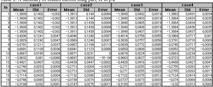
Table 2. A summary of branch current imag part, Ix in p.u... 39
Table 3. Case1-1 summation of load in switch zone ... 63
Table 4. Case 1-1 meter difference in meter zone... 63
Table 5. Case 1-1 topology error detection result... 63
Table 6. Case 1-2 summation of load in switch zone ... 63
Table 7. Case 1-2 meter difference in meter zone... 64
Table 8. Case 1-2 topology error detection result... 64
Table 9. Case 2-1 summation of load in switch zone ... 64
Table 10. Case 2-1 meter difference in meter zone... 64
Table 11. Case 2-1 topology detection result... 65
Table 12. Case 2-2 summation of load in switch zone ... 65
Table 13. Case 2-2 meter difference in meter zone... 65
Table 14. Case 2-2 topology error detection result... 65
Table 15. Case 1 topology error detection result when node 9 open... 67
Table 16. Case 2 topology error detection result when node 9 open... 68
Table 17. Case 1 SCB error detection when SCB 10 open... 69
LIST OF FIGURES
Figure 1. A three-phase line section... 15
Figure 2. One-line diagram of reduced feeder ... 20
Figure 3. Branch Current Estimation for Case 1 and Case 2... 22
Figure 4. Branch Current Estimation for Case 3 and Case 4... 23
Figure 5. One-line diagram of reduced feeder ... 38
Figure 6. Currents error for Case 1 and Case 2 from Monte Carlo simulation ... 40
Figure 7. Currents error for Case 3 and Case 4 from Monte Carlo simulation ... 41
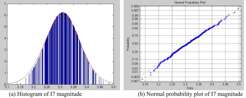
Figure 8. Normality check of I7 magnitude for case 3 ... 43
Figure 9. Normality check of I7 magnitude for case 4 ... 43
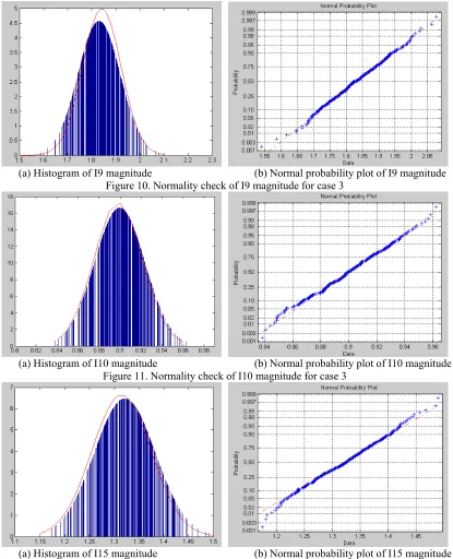
Figure 10. Normality check of I9 magnitude for case 3 ... 44
Figure 11. Normality check of I10 magnitude for case 3 ... 44
Figure 12. Normality check of I15 magnitude for case 3 ... 44
Figure 13. Normality check of I17 magnitude for case 3 ... 45
Figure 14. Sum of Square Error Plot in four cases ... 46
Figure 15. Quality of the estimates in four cases ... 47
Figure 16. No. of bias point in case 1 and case 4... 48
Figure 17. Quality of the estimates in case 1 and case 4... 49
Figure 18 Sum of Square Error in four cases in 5000 Monte Carlo simulations... 49
Figure 19 Quality in four cases in 5000 Monte Carlo simulations ... 50
Figure 20. Zone defined by switches and meters in a feeder ... 55
Figure 21. Flowchart of Method I Algorithm ... 56
Figure 22. Flowchart of Method II Algorithm... 60
Chapter 1
Introduction
1.1
Background
Our literature indicates that utilities have been improving their means of monitoring their
distribution systems mainly to improve service reliability [1-6, 10, 12]. Recently, there has
been an additional incentive to advance the monitoring of feeders – the improvement of
efficiency by adopting advanced functions such as voltage control for demand management.
Effective management of distribution systems requires analysis tools that can estimate the
state of the system (the operating condition) and predict the response of the system to
changing load and weather conditions. The main tool used for system analysis is power flow
analysis. But this tool is not very suitable for real-time monitoring as it requires accurate load
and system data.
In order to better monitor the system operating conditions for system management, some
utilities have begun the installation of limited Supervisory Control And Data Acquisition
(SCADA) systems at the distribution level. Additionally, some utilities have deployed large
scale Advanced Metering Infrastructures (AMI). With the availability of real-time
distribution system. One of the approaches is power flow based [4-6, 12] and the others [2, 3]
are extensions of the conventional state estimation (SE) method for three-phase analysis.
Although SE is preferred over the power flow approach, its computational complexity may
prevent its use in practical applications.
In this thesis, a branch-current-based three-phase SE (BCSE) method [1] is considered, as
it is computationally more efficient and less sensitive to line parameters than the
conventional node-voltage-based SE methods. BCSE is very efficient in handling line-flow
and power-injection measurements for radial networks. In the original algorithm, the voltage
measurements have not been available [1]. But with AMI, voltage measurements will be
readily available. In this thesis, we show the enhancement of the original BCSE to include
more accurate voltage measurements.
Computer simulations such as power flow studies give exact answers, but in reality we
never know the absolutely true state of a physical operating system. Even when great care is
taken to ensure accuracy, unavoidable random noise enters into the measurement process to
distort more or less the physical results. However, repeated measurements of the same
quantity under carefully controlled conditions reveal certain statistical properties from which
the true value can be estimated. Thus, statistical technique is necessary to the process of
determining the correctness of an SE implementation [16, 17].
In this thesis, some statistical techniques are presented for assessing the BCSE
performance. Because of the statistical nature of pseudo measurements, the performance of
the SE needs to be assessed through statistical measurements. In this manner, it is essential to
The SE application relies on the basic assumption that the topology of the system is
known beyond any doubt [21-24]. However, in most of the real world situations, the state of
some switching devices is unknown or, for some reason, the current value in the database is
under suspicion. If a circuit breaker or a switch is a part of the modeled network but is not
monitored by SCADA, its open/close position in the database is updated manually by the
power system dispatchers. In many system maintenance jobs, after a series of manually
directed switching operations, the dispatcher often forgets to update the open/close positions
of these switches. The result of this situation is a topology error in the network. Model
topology errors can also occur when the telemetered circuit breaker ON/OFF status is
incorrect.
Correct connectivity in power network modeling is so critical to modern market and
security operations that topology estimation is expected to become a standard EMS function.
Therefore, topology error identification and detection algorithm using BCSE method is
proposed in this thesis.
1.2
Thesis Objective
The main objective of this thesis is to improve upon BCSE method using the availability
of voltage measurements with the adoption of AMI technologies in the distribution system.
Original BCSE method is a suitable algorithm to solve distribution state estimation and is
designed to include only power and current measurements. However, because of its
complexity, voltage measurement has been ignored. Thus, the enhancing of BCSE extended
different measurement are considered to assess the impact of voltage measurements on the
BCSE method.
Furthermore, some statistical techniques are presented using the results obtained from the
enhancement of the BCSE method. Performance measures are adopted to evaluate the
enhanced BCSE method. For these measures, Monte Carlo simulation is performed in
enhancing BCSE method to compute their results by repetitive random sampling.
The third objective is to describe an approach by which the circuit breaker status error
can be detected and identified in the presence of analog measurement error using the BCSE
method. The use of normalized residuals from the result of the BCSE method is proposed for
the detection of topology errors. Two types of topology error are considered : switching
device error and shunt capacitor bank error.
For testing the revised BCSE, a reduced version of IEEE 34 node radial test feeder is
used. The simulation platform used in this study is developed using C language on Microsoft
Visual Studio .NET 2003.
1.3
Related Work
Distribution systems consist mainly of feeders. The feeder has characteristics such as
radial, weekly meshed etc. Although the main feeder is the three-phase backbone of the
circuit, branching from the mains are one or more lateral branches which can be single and
two-phase rather than three-phase. Furthermore, the loads on the feeders can be single and
Distribution systems provide very few real-time measurements. The most common
measurement type is power which is available only at the substation and only measures
current magnitude. While few voltage magnitude measurements are obtained, they are more
accurate. Because of a lack of real-time data, pseudo measurements, primarily obtained from
historical load data and customer billing data are substituted. Therefore, performing high
efficiency SE with minimal real-time data is a challenging task [2, 4].
A Distribution SE has a critical role in the Distribution Management System (DMS) for
estimating unknown states which provide limited measurement information. For reliable and
optimal DMS control, several DSE methods have been proposed. There are two main
approaches in SE. one is the algorithm based on power flow [4-6] and the others are
Weighted Least Square (WLS) based [1-3]. Because of the complexity of computation in the
power flow approach, its use may be unwieldy in the practical power flow approach, and it
may prevent use in practical power systems. In this paper, for efficient calculation, BCSE
method is used [1].
BCSE is very efficient in handling line-flow and power-injection measurements for radial
networks. In the original algorithm the voltage measurements were not available. But with
AMI, voltage measurements will be readily available. In paper [9], the method for handling
voltage measurements in BCSE method is introduced. This method converts the voltage
measurements into equivalent measurements. In addition, in paper [11], an algorithm for
treating power and current measurements with the BCSE method is proposed using the same
Statistical technique is the suggested process for determining the correctness of an SE
implementation. For this purpose, Monte Carlo simulation is one of the key devices to assess
SE simulation. However, the disadvantage is the computer time required to achieve the
acceptable accuracy of the estimator. In general, the Monte Carlo process is repeated until
interesting quantities are within the range expected. In papers [13, 19, 20], an approximate
procedure that is able to determine, with very few iterations, the total number of runs
required to obtain desire accuracy.
Furthermore, in [18], the statistical test used for hypothesis testing to make statistical
decisions is introduced. The goal of this statistical test is to ensure the accuracy of the quality
of state estimation. This paper examines a number of hypothesis testing problem settings for
multivariate data. For the parametric test, Hotelling’s 2
T test is used while for the
nonparametric test, multivariate sign test and sign rank test are employed.
It is important to have a test method that gives assurances that the measurement increase
or the type of measurement in the state estimation reflects true improvement in the
performance. Regarding this issue, the paper [16, 17] introduced performance evaluation to
assess the effectiveness of WLS through certain statistical measures including bias,
consistency and quality of the estimates.
The SE application relies on the basic assumption that the topology of the system is
known beyond any doubt. Since most of the switching in a distribution system is done
manually and not telemetered, SE can help the dispatchers keep the network topology
As another approach, the use of normalized residuals from the result of the SE method is
proposed for the detection of topology errors. When a topology error happens, the bus/branch
model generated by the topology process is locally incorrect, causing a topological error.
Unlike the parameter errors where threshold is exceeded, topology errors usually cause the
state estimate to be significantly biased. As a result, the bad data detection & identification
routine may erroneously eliminate several analog measurements which appear as interacting
bad data, finally yielding an unacceptable state. Therefore there is a need to develop effective
mechanisms intended to detect and identify these types of gross errors [25].
1.4
Thesis Outline
• Chapter 2
This Chapter considers the incorporation of voltage measurements in Branch Current
State Estimation (BCSE) programs. Originally, the BCSE was designed to include only
power and current measurements. The motivation for enhancing BCSE is that with the
adoption of large scale automated meter infrastructure (AMI) technologies, voltage
measurements will be available at the distribution level. Including these measurements has
the potential to improve the accuracy of the state estimation. The Chapter elaborates the
technical approach taken to accomplish this task, and the test results for assessment.
• Chapter 3
This chapter presents a statistical technique to assess the BCSE performance. Because
assessed through statistical measurements. Some statistical measures quantified in terms of
bias, consistency, and quality are adopted to evaluate the enhanced BCSE method. For
statistical analysis, 300 Monte Carlo simulations are performed.
• Chapter 4
This Chapter describes the topology error identification algorithm in a Branch Current
State Estimation (BCSE) program. BCSE application relies on the basic assumption that the
topology of the system is known beyond any doubt. However, in most real world situations,
the state of some switching devices is unknown or, for some other reason, the current value
in the database is under suspicion. In this Chapter, two approaches are described to address
topology identification problem in the scope of state estimation.
• Chapter 5
Overall conclusion and future work.
1.5
Glossary
In this master thesis, the following abbreviations and terms are used :
AMI : Automated Meter Infrastructure is an intelligent technology that includes metering
systems capable of recording and reporting energy consumption and other measurements at
BCSE : Branch Current State Estimation algorithm, like conventional node-voltage-based
SE methods, is based on the weighted least square approach. Rather than using the node
voltages as the system state, the method used the branch currents as the state.
CB : Circuit Breaker is an automatically-operated electrical switch designed to protect an
electrical circuit from damage cased by overload or short circuit.
EMS : Energy Management System, which is used in the monitoring and control of the
power generation and transmission.
IEEE : Institute of Electrical and Electronics Engineering
LF : Load Flow analysis is in the planning the future expansion of power systems as well as
in determining the best operation of existing systems. The principal information obtained
from the load flow study is the magnitude and phase angle of the voltage at each bus and the
real and reactive power flowing in each line.
P.U. : Per Unit system is the expression of system quantities as fractions of a defined base
unit quantity in electrical engineering in the field of power transmission.
SCADA : Supervisory Control And Data Acquisition systems are used to monitor and
control power system in a wide range of applications like power station control, transmission,
distribution automation.
SCB : Shunt Capacitor Banks are mainly installed to provide capacitive reactive
compensation/power factor correction.
SE : State Estimation as a mathematical analysis tool acts as a noise filter to eliminate errors
available, but they cannot be used in conventional power-flow calculations. these limitations
can be removed by state estimation.
SW : Switch is an electrical component which can break an electrical circuit, interrupting the
current or diverting it from one conductor to another.
WLS : Weighted Least Square state estimation algorithm. Commonly, this algorithm is
based on the assumption that the measurement errors have normal distributed noises with
Chapter 2
Including Voltage Measurements in
Branch Current State Estimation for
Distribution Systems
2.1
Overview
BCSE is tailored to perform state estimation on distribution networks. There are a
number of significant differences in the characteristics of typical distribution networks
compared to typical transmission networks.
Distribution systems consist mainly of feeders. Feeders are mainly radial, but have
laterals that can be single or two-phase rather than three-phase. Furthermore, loads on the
feeders are more distributed than that of the transmission and these loads can be single and
two-phase (for residential service) or three phase (for commercial and industrial service).
Therefore, distribution systems are unbalanced in nature. Also, feeder line sections are
So, to obtain the consistent and accurate data, new methods are proposed for monitoring
and operation of distribution system. One of the approaches is power flow based [2] and the
others [3,4] are extensions of the conventional state estimation (SE) method for three-phase
analysis. Although SE is preferred over the power flow approach, its computational
complexity may prevent its use in practical applications. In this paper, for efficient
calculation A branch-current-based three-phase SE (BCSE) method [1] is used.
The method is computationally more efficient and more insensitive to line parameters
than the conventional node-voltage-based SE methods. The method has superior performance
both in terms of computational speed and memory requirements. Furthermore, the method is
insensitive to line parameters, which improves both its convergence and bad data handling
performance. The BCSE method, like conventional node-voltage-based SE methods, is based
on the weighted least square (WLS) approach.
BCSE is very efficient in handling line-flow and power-injection measurements for radial
networks. However, handling voltage measurements increases the complexity of the
algorithm, as using the branch currents as state variables makes the treatment of voltage
measurements difficult.
Power system state estimation relies on measurement data obtained from substations and
on topological model. A practical SE must possess the ability to handle power, current and
voltage measurements efficiently. Although a distribution system does not have an
overwhelming number of voltage measurements, they are often found in the telemetry of a
measurements. So, one of the main focus of this project is to develop a BCSE method with
power, current magnitude and voltage magnitude measurements.
2.2
State Estimation
State estimation (SE) as a mathematical analysis tool acts as a noise filter to eliminate
errors in data. The acquired data always contains inaccuracies which are unavoidable since
physical measurements cannot be entirely free of random errors or noise. Because of noise,
the true values of physical quantities are never known and we have to consider how to
calculate the best possible estimates of the unknown quantities. The method of least squares
is often used to “best fit” measured data relating two or more quantities.
2.2.1
The Weighted Least Square (WLS) Approach
The SE method is based on the weighted least square (WLS) approach. WLS is useful
for estimating the values of model parameters when the response values have differing
degrees of variability over the combinations of the predictor values. Mathematically, WLS
find the best estimates which are chosen as those which minimize the weighted sum of the
squares of the measurements errors. WLS state estimation tries to find a system state,
2 1
( ) m ( ( )) [ ( )]T [ ( )]
i i i
x
i
f m i n J x w z h x z h x W z h x
=
= =
∑
− = − − (2. 1)where wi and hi represent the weight and the measurement function associated with
measurement zi respectively. For the solution of this optimization problem gives the
estimated state xˆ which must satisfy the following optimality condition:
( ) 0
i f f x x ∂ Δ = =
∂ (2. 2)
1
( ) 2 m ( ( )) i 0
i i i
i
i i
h x f
w z h x
x = x
∂ ∂ = ⋅ − ⋅ = ∂
∑
∂[ ][
]
1 ( )( ( )) ( ) 0
m
T i
i i i
i i
h x
w z h x H W z h x
x
=
∂ ⎡ ⎤
= − ⋅ =⎣ ⎦ − =
∂
∑
(2. 3)where H x( ) h x( )
x ∂ =
∂ is the Jacobian matrix of the measurement function ( )h x . Since ( )h x is
usually non-linear, the solution is obtained by an iterative method. The iterative method
involves solving the linear equation of the following type at each iteration to compute the
correction k 1 k k
x + =x ++x .
( 1) ( ) ( )
ˆ ˆ
( k k ) T [ ( k )]
G x + x H W z h x
⇒ − = − (2. 4)
where d x( )ˆ T
H WH G
x
∂ = − = −
∂
is the jacobian of the optimality condition equation :
ˆ
( ) T [ ( )]
d x =H W z−h x (2. 5)
One of the main challenges in implementing this approach for SE in distribution feeders is
incorporating the unbalanced nature of distribution feeders into the problem. The most
2.2.2
Feeder Representation
In general, main feeders are three-phase, however some laterals can be two-phase or
single-phase. The lines are usually short and un-transposed. Loads can be three-phase,
two-phase or single-two-phase (like residential customers). Therefore it is desirable to use a three
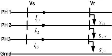
phase model as also recommended for power flow analysis of feeders. A three-phase line
model takes into account the magnetic coupling between the phases in lines, which for a line
section ,l l=1"b, such as the one shown in Fig.1, is of the following form
,1 ,1 11 12 13 ,1
,2 ,2 21 22 23 ,2
,3 ,3 31 32 33 ,3
r S l
r S l
r S l
V V z z z I
V V l z z z I
V V z z z I
⎡ ⎤ ⎡ ⎤ ⎡ ⎤⎡ ⎤
⎢ ⎥ ⎢= ⎥− ⎢ ⎥⎢ ⎥
⎢ ⎥ ⎢ ⎥ ⎢ ⎥⎢ ⎥
⎢ ⎥ ⎢ ⎥ ⎢⎣ ⎥⎦⎢ ⎥
⎣ ⎦ ⎣ ⎦ ⎣ ⎦
(2. 6)
or Vr =VS −Z Il l
where Zl =g Zl is the line impedance matrix and gl is the line length. Note that this equation
is written for the assumed branch current direction shown in Fig 1, and the phases are
numbered as ϕ =1, 2,3 rather than labeled as a,b,c.
2.2.3
Branch-Current-Based on State Estimation
The branch-current-based SE method, like conventional node-voltage-based SE
methods, is based on the weighted least square (WLS) approach. Rather than using the node
voltages as the system state x, the method uses the branch currents and solves the following
WLS problem to obtain an estimate of the system operating point defined by the system state
x :
2 1
( ) m ( ( )) [ ( )]T [ ( )]
i i i
x
i
m i n J x w z h x z h x W z h x
=
=
∑
− = − − (2. 7)where wi and ( )h xi represent the weight and the measurements function associated with
measurement zi respectively. For the solution of this problem the conventional iterative
method is adapted by solving following normal equations at each iteration to compute the
correcting k 1 k k
x + =x ++x
[ ( )]k k T( ) [k ( )]k
G x Δ =x H x W z−h x (2. 8)
where
( ) T( ) ( )
G x =H x WH x (2. 9)
is the gain matrix and H is the Jacobian of the measurement function ( )h x .
Hence the only difference between the node voltage based SE and BCSE is the measurement
functions associated with the type of measurements to be processed. To illustrate these
functions for BCSE, consider two cases
Case 1: power flow (P, Q) or current magnitude (I) measurements on a line section of a
feeder
Case 1 – power flow (P, Q) or current magnitude (I) measurements:
Power measurements in BCSE are converted to equivalent complex current
measurement by using the current estimate of the node voltage:
2 2
m m
m r x
r
r x
P V Q V I
V V
+ =
+ , 2 2
m m
m x r
x
r x
P V Q V I
V V
− =
+ (2. 10)
Hence the resulting measurement functions are linear as the state variables are the complex
branch currents,
l lr lx
I =I + jI , l=1..n (2. 11)
The current magnitude measurements, on the other hand are non-linear, as
2 2
lx lr
l I I
I = + (2. 12)
The current magnitude measurements introduce coupling terms between the real and
imaginary parts. For example, the current measurement m l
I introduces the following non-zero
elements into the measurement Jacobian H
cos m I r h I φ ∂ =
∂ , sin
m I x h I φ ∂ =
∂ (2. 13)
where 1
, tan ( , / , )
lϕ Ixlϕ Irlϕ
φ = −
Case 2 –Voltage magnitude (V) measurements:
A voltage at the node t of a radial feeder Vt is the voltage at the substation minus the
voltage drop on the line sections between the substation and this node, and hence, the
measurement function for the voltage measurement Vt can be written in terms of the branch
m
t S l l
V =V −
∑
Z I (2. 14)The voltage magnitude measurements introduce coupling terms between the phases of branch
currents and the real and imaginary parts of branch currents. The voltage measurement Vt
introduces the following non-zero elements into the measurement Jacobian H
,
, ,
sin cos
m Vl
l l l l
rl h X R I ϕ ϕ ϕ φ φ ∂ = − ∂ , , , , sin cos m Vl
l l l l
xl h R X I ϕ ϕ ϕ φ φ ∂ = − −
∂ (2. 15)
where Zl =Rl + jXlis line impedence and VS =VSR+ jVSXis substation voltage
1
1 1
( SR ( m j j) / SX ( m j j))
j j
Tan V real Z I V imag Z I
φ −
= =
= −
∑
−∑
(2. 16)Hence, both the Jacobian H and the gain matrix G are revised to include voltage
measurements in BCSE.
2.2.4
BCSE Algorithm
BCSE constructs the Jacobian and gain matrices and solves the update equations of ()
iteratively. The algorithm involves the following steps at each iteration k :
Step 1 - Given the node voltage k 1
V − , convert power measurements into equivalent current
measurements
Step 2 - Use current measurements to obtain an estimate of branch currents [ , , ]
k k k
r x
xϕ = I ϕ I ϕ
by solving the update equations (1) for each phase ϕ = 1,2,3
Step 3: Given the branch currents, update the node voltages k
V by the forward sweep
Step 4: Check for convergence; if two successive updates of branch currents are less than a
convergence tolerance then stop, otherwise go to step 1
2.3
State Estimation Test Results
For testing the revised BCSE with voltage measurements, a test feeder is used. The test
feeder is a 34 bus, 23kV, 3-phase radial IEEE test feeder [5]. A reduced version of this test
feeder is used to facilitate debugging and assessment. A one-line diagram of the feeder is
given in Fig. 2 with the nodes renumbered to make the illustration of the results easier. The
feeder is predominantly three-phase with some single-phase laterals and has both spot and
distributed loads. For test purpose, distributed line section loads are lumped equally at
terminal nodes of the line section. The nominal load data is taken as the actual load and the
power flow results are used to determine the correct measurements for this load. The
minimum voltage for this loading is
min 21,a 0.9402 3.057
V =V = ∠ −
which indicates a heavy loading condition on the feeder. The line data used is given in [6]
with line r/x ratios varying between 0.57 and 1.37.
For SE, the available measurements assumed are given in the figure also: voltage and power
flow at the substation, current measurements on branches 6-7, and voltage measurements on
0
1 2 3 4 5 6 7 8 15 16
17 10 9 11 12 14 Meter (power) Meter (current) Meter (voltage)
m0 m1 m2
m4
13
m3
Figure 2. One-line diagram of reduced feeder
To generate measurement data for testing purpose, first the actual measurements have
been obtained by running a power flow for the given load. Then measurement error was
added to the actual measurements.
a Z
Z =Z ±e (2. 17)
where a
Z is actual data and eZ is the measurement error. The forecasted load data is created
by perturbing the actual load data by adding error of 30%. The power and current magnitude
measurement errors are selected from Normal distribution with a standard deviationσ of
0.0233 (accuracy is 7% of their measured values). The voltage measurements data are
generated by adding measurement error with a standard deviation σ of 0.0067 (2%
measurement error). The weights are obtained by using standard deviation σ of
measurements error. 2 1 i i w σ
= (2. 18)
where wi and σi represent weight associated with measurement ziand standard deviation of
measurement error, respectively. The revised algorithm was implemented using the C
language on Microsoft Visual Studio .NET 2003. To assess the impact of voltage
Case 1: forecasted load data.
Case 2: The same measurements as in Case 1 plus three voltage measurements m2-m4 from
the feeder nodes.
Case 3: Power measurement at the substation (both real and reactive), indicated as mo in Fig.
2, plus a current measurement on the feeder, m1, and forecasted load data.
Case 4: The same measurements as in Case 3 plus three voltage measurements m2-m4 from
the feeder nodes.
The enhanced BCSE has run for these four cases. For these simulations, the addition of
voltage measurements do not affect the convergence of the method; it takes about 3-6
iterations for the solution to converge. This indicates that BCSE’s computational
performance does not degrade with the addition of voltage measurements.
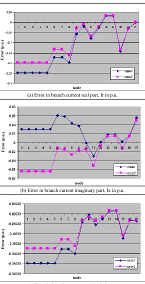
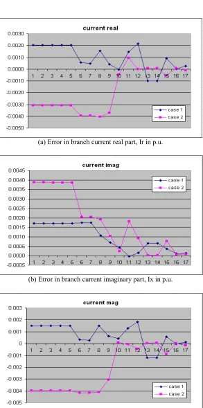
Test results are given in the Appendix I. A summary of the results are given in Fig. 3-4 for
the four cases considered. The figures show the error in the estimated state (x=[ , ]Ir Ix ) of
phase a branch currents on the feeder. Fig. 3 compares the results for Case 1 and Case 2.
These results indicate that adding voltage measurements decrease the error in branch current
estimates. Note that the improvement in the estimation is more on the real part of the current
than the imaginary part. Since, in this case the currents have small imaginary component, the
overall reduction of the error in the current magnitude is considerable especially towards the
substation end of the feeder. Hence, these results indicate that having voltage measurements
helps improve the estimation over the conventional one that is based on the forecasted load
(a) Error in branch current real part, Ir in p.u.
(b) Error in branch current imaginary part, Ix in p.u.
(c) Error in branch current magnitude in p.u. Figure 3. Branch Current Estimation for Case 1 and Case 2
node
Error
(p
.u
.)
node
Error
(p
.u
.)
node
Error
(p
.u
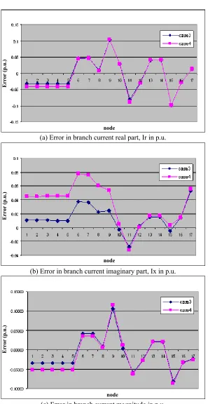
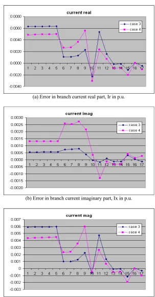
(a) Error in branch current real part, Ir in p.u.
(b) Error in branch current imaginary part, Ix in p.u.
(c) Error in branch current magnitude in p.u. Figure 4. Branch Current Estimation for Case 3 and Case 4
node
Error
(p
.u
.)
node
Error
(p
.u
.)
Error
(p
.u
.)
Figure 4 compares the results for Case 3 and Case 4. Note that these two cases illustrate the
effect of adding voltage measurements to a system which has some limited power and current
measurement from the feeder (Case 3). The results indicate that in this case adding voltage
measurements does not improve the estimation as much as it did in the previous case. The
differences between the two cases are not statistically significant.
2.4
Conclusions
This chapter shows that the basic BCSE can be extended to include voltage
measurements in the estimation. The initial test results indicate that the impacts of the
voltage measurements on the estimated values are marginal. These results are based on the
simulated measurement with assumed accuracy on especially the load forecast values. The
method however now allows including the voltage measurements in actual applications in
Chapter 3
Performance of Branch Current State
Estimation Method
3.1
Overview
In the previous chapter, the enhancement of the original BCSE to include voltage
measurements is described. Because of the statistical nature of pseudo measurements, the
performance of the BCSE needs to be assessed through statistical measurements. Thus, this
chapter looks at the performance of enhanced BCSE method in the presence of measurement
noises through Monte Carlo simulation.
Singh and others have proposed some statistic measures quantified in terms of bias,
consistency, and quality through Monte Carlo simulation in [17] for assessing the quality of
state estimation. In this chapter, these performance measures are adopted to evaluate the
enhanced BCSE method.
3.2
Monte Carlo Simulation
Monte Carlo simulation is used to estimate expected values of random variables when it
Carlo methods are a class of computational algorithms that rely on repeated random sampling
to compute their results. Monte Carlo methods are often used when simulating physical and
mathematical systems. Because of their reliance on repeated computation and random or
pseudo-random numbers, Monte Carlo methods are most suited to calculation by a computer.
Monte Carlo methods tend to be used when it is infeasible or impossible to compute an exact
result with a deterministic algorithm.
Monte Carlo simulation methods are especially useful in studying systems with a
large number of coupled degrees of freedom. Furthermore, Monte Carlo methods are useful
for modeling phenomena with significant uncertainty in inputs, such as the calculation of risk
in business. Furthermore, the basic characteristics of Monte Carlo simulation is described :
▪ Monte Carlo simulation allows several inputs to be used at the same time to create the
probability distribution of one or more outputs.
▪ Different types of probability distributions can be assigned to the input of the model. When
the distribution is unknown, the one that represents the best fit could be chosen.
▪ The use of random numbers characterized Monte Carlo simulation as a stochastic method.
The random numbers have to be independent; no correlation should exist between them.
▪ Monte Carlo simulations generate the output as a range instead of a fixed value and shows
how likely the output value is to occur in the range.
In general, the Monte Carlo simulation involves the following series of steps [15].
Step 1 – Construct a simulated “universe” of some randomizing mechanism whose
composition is similar to the universe whose behavior we wish to describe and investigate.
Step 2 – specify the procedure that produces a pseudo-sample which simulates the real-life
sample in which we are interested. That is, specify the procedural rules by which the sample
is drawn from the simulated universe. These rules must correspond to the behavior of the real
universe in which we are interested. To put it another way, the simulation procedure must
produce simple experimental events with the same probabilities that the simple events have
in the real world.
Step 3 – If several simple events must be combined into a composite event, and if the
composite event was not described in the procedure in step 2, describe it now.
Step 4 – Calculate the probability of interest from the tabulation of outcomes of the
resampling trials.
3.2.1
Monte Carlo Simulation Sample Size [15]
Monte Carlo simulation is used to estimate quantities in such as :
- The bias and variance of an estimator
- The percentiles of a test statistic or pivotal quantity
- The power function of a hypothesis test
- The mean length and coverage probability of a confidence interval
In this manner, Monte Carlo simulation sample size can be defined depending on which
quantities are interested [15].
• Bias Estimation
1 N i i x x N =
=
∑
(3. 1)and the standard deviation of sample is
N
σ
where 2 var( )
x
σ = . So given a guess of σ , say
σ, and an acceptable value, say d, for the standard deviation of our estimate, the sample
size for bias estimation is defined as :
2 2
N d
σ
= (3. 2)
• Variance Estimation
The sample variance is :
1 2 2 1 ( ) 1 N N i i x x S N − = − = −
∑
(3. 3)For large N, the approximate variance of the sample variance will be close to
4( ( ) 1) /
Kurt x N
σ − , where 2 var( )
x
σ = and Kurt x( )is the kurtosis of the distribution of x.
Many estimators are approximately normal provided the sample size is not too small. So, the
approximate standard deviation of the variance estimation is 2 / 2
N ⋅σ . For acceptable d,
the sample size for variance estimation is defined as :
4 2 2 N d σ
= (3. 4)
• Power Estimation
For a new test procedure of the form “reject the null hypothesis if T >cα”, the power at a
n 1 1 ( ) N i i
pow I T c
N = α
=
∑
> (3. 5)where Ti is the test statistic for the i-th Monte Carlo sample, cαis a given critical values, and
I is the indicator function having value 1 if Ti >cα and 0 otherwise. This is binomial
sampling, and the worst variance of our estimate (occurring at power ½) is given by 1/(4 )N .
Setting d =1/(2 N) yields
2
1 4
N d
= (3. 6)
• Confidence Intervals
Coverage probability and average confidence interval length are both important quantities
that should be reported whenever studying confidence intervals. Obviously we would like
intervals that achieve the nominal 1−α coverage (like 95%) and are short on average. For sample size considerations, we need a preliminary estimate σ of the standard deviation of the lengths and an acceptable value dfor the standard error of our estimate of average length.
Then just Eq. 3.3 is obtained. For coverage estimation or one-sided error estimation, it is
inverted to d (1 )
N
α −α
= where dis the acceptable standard deviation for coverage estimate,
to get 2 (1 ) N d α −α
= (3. 7)
3.2.2
Monte Carlo Simulations on BCSE Method
Step 1 – BCSE method tries to find a system state, represented by xˆ, by minimizing the
weighted sum of the squares of the measurements errors.
Step 2 – First the actual measurements have been obtained by running a power flow for the
given load. Then measurement error obtained from random generator based on Normal
distribution was added to the actual measurements.
a Z
Z =Z ±e (3. 8)
where a
Z is actual data and eZis the measurement error. The forecasted load data is created
by perturbing the actual load data by adding error of 30%. The power and current magnitude
measurement errors are selected from Normal distribution with a standard deviationσ of
0.0233 (accuracy is 7% of their measured values). The voltage measurements data are
generated by adding measurement error with a standard deviation σ of 0.0067 (2%
measurement error).
Step 3 – The sample size is defined in order to achieve acceptable results. In this thesis, 300
Monte Carlo simulations have been chosen.
Step 4 – To calculate the probability of the interest, the estimated states (x=[ , ]Ir Ix ) of
branch currents are obtained and then, hypothesis testing is adopted to test the bias in
estimated state variables. Furthermore, the performance measures which are bias, consistency
and overall quality are examined.
In order to achieve acceptable results obtained from Monte Carlo simulation, the
sample size is defined in the previous section. However, this determination can be only
BCSE method, we need another sample size determination. In BCSE method, we performed
both parametric and nonparametric test for the bias test. For parametric tests, Hotelling’s 2
T
test is used and as with the nonparametric test, multivariate sign test and sign rank tests are
applied. In Hotelling’s 2
T test, sample size is enough if the following condition is satisfied :
2
1 0
T
p − ≈ (3. 9)
where 2
T and p is Hotelling’s T2 test statistics value and number of state, respectively.
Similarly, the enough sample size can be defined in multivariate sign test and sign rank tests
to achieve acceptable accuracy of the result.
For the multivariate sign test, the following condition is satisfied.
2
1 0
Q
p − ≈ (3. 10)
where 2
Q and p is sign test statistics value and number of state, respectively.
For the multivariate sign rank test, the following condition is used to check the suitable
sample size.
2
1 0
U
p − ≈ (3. 11)
where 2
U and p is sign rank test statistics value and number of state, respectively.
3.3
Bias in BCSE Method
Since we have N state (x=[ , ]Ir Ix ) of branch currents, we need to perform multivariate
number of hypothesis testing problem settings for multivariate data in [18]. In this chapter,
hypothesis testing is adopted to test the bias in estimated state variables obtained from BCSE
method.
3.3.1
Multivariate Statistical Tests
One of the most important problems in the area of multivariate analysis is to obtain
the mean vector of the given sample. After that, we can get rough information about the
population where the sample is surveyed. Often people may hope to test the hypothesis
whether the sample mean vector equals to the specified value in advance. For this, there are
two typical approaches, parametric test and nonparametric test. Most hypothesis tests are
based on the assumption that random samples are from normal populations. This is called a
parametric test because it is based on a particular parametric family of distributions.
Alternately, these procedures are not distribution-free because they depend on the assumption
of normality. The primary advantage of the parametric test is that it has greater statistical
power to detect differences. The other approach is called a nonparametric test which has no
assumptions about the distribution of the underlying population other than that it is
continuous. One of the advantages is that the data need not be quantitative but can be
categorical or rank data. In SE problems, the assumptions for the parametric test may be
difficult or impossible to justify so that both parametric and nonparametric tests are
performed. For parametric tests, Hotelling’s 2
T test is used and as with the nonparametric test,
3.3.2
Multivariate Parametric Tests [18]
Let x x1, , ,2 " xN be independent and identically distributed from (F x−θ), where
( )
F ⋅ represents a continuous p-dimensional distribution “located” at the vector parameter
1 2
( , , , )T p
θ = θ θ " θ . The hypothesis whether the sample mean vector equals to the vector
specified in advance is :
0: a:
H θ μ= H θ μ≠ (3. 12)
Note the above hypothesis is equivalent to :
0: 0 a: 0
H θ μ− = H θ μ− ≠ (3. 13)
Hotelling’s 2
T test statistics involves the following calculations.
2 ( ) 1( )
T =N x−μ ′S− x−μ (3. 14)
where
x : the mean vector of sample, ave x{ }i
N : the sample size.
S : the sample covariance matrix, ave x{( i−x x)( i−x) }T μ : the vector given in the hypothesis.
2 1 N T N p −
− has F distribution with degrees of freedom, pandN−p. Thus given significant
level is α , the null hypothesis is rejected when :
2
,
1
( )
p N p
N
T F
N p − α
− ≥
where Fv v1, 2( )α is the upper α th quantile of an F distribution with v1and v2degrees of freedom.
Moreover, the p-value for this test statistics is :
2
1 , ,
( 1)
N p
p value F T p N p
N p
⎛ − ⎞
− = − ⎜ ⋅ − ⎟
−
⎝ ⎠ (3. 16)
3.3.3
Multivariate Nonparametric Tests [18]
For the nonparametric test, multivariate sign test and signed rank test are used. As for
the sign test, spatial sign function is defined as :
( )
i x i
S =S A x for i=1,"N (3. 17)
where Axis transformation proposed by Tyler. Basically, Tyler’s shape matrix Vx is positive
definite symmetric p×pwith trace equals p. Thus, for any Axwith A ATx x =Vx−1
{ T}
i i p
p ave S S⋅ =I (3. 18)
Tyler’s transformation matrix Ax makes the sign covariance matrix equal to 1 Ip
p , the
variance-covariance matrix of a vector that is uniformly distributed on the unit psphere. Due
to the fact that Siand −Si give the same contribution to the sample covariance matrix,
x
A could be considered as the method to make the direction of transformed data points ±A xx i.
The sign test rejects null hypothesis for large
2
2 T
For large sample size, underlying distribution is directionally symmetric and null hypothesis
holds, 2
Q has approximate χ2p . Therefore, we should reject null hypothesis in favor of
alternative hypothesis with the condition :
2 2
p
Q ≥χ (3. 20)
For the multivariate rank test, we first use the signs of transformed differences :
( ( ))
ij x i j
S =S A x −x (3. 21)
This makes the centered rank :
( )
i j ij
R =ave S (3. 22)
and the average of Ri is zero. In multivariate case, the data based transformation Axis
selected to make the rank procedure affine invariant. So the transformation is chosen to
satisfy the follow :
( T) ( T )
i i i i p
p ave R R⋅ =ave R R I (3. 23)
This transformation then leads the rank covariance matrix equivalent to a number times the
identity matrix, that is :
2
( T) x
i i p
c
ave R R I
p
⎛ ⎞
= ⎜ ⎟
⎝ ⎠ (3. 24)
Through the theoretical analysis, we get the test statistics as :
2 2
2 ( ( ( )))
4 x i j
x
Np
U ave S A x x c
If random sample is form and elliptically symmetric distribution with symmetry center θ =0,
then we have 2
U has an approximate chi-square distribution with degree of freedom p. So
we would reject the null hypothesis if
2 2( ) p
U ≥χ α (3. 26)
3.4
Performance of BCSE Method
The performance measures are bias, consistency and overall quality. These concepts
of statistical techniques are illustrated and used in this chapter [17].
3.4.1
Bias
State vector, xˆ is an unbiased estimate of true state vector, xt if the expected value of
ˆ
xis equal to xt.
ˆ
( ) t
E x =x (3.27)
This is equivalent to saying that the mean of the probability distribution of xˆ is equal to xt.
3.4.2
Consistency
If ˆxN is an estimator of xt based on a random sample of N observations, ˆxN is
consistent for xt in this condition :
ˆ
lim ( N t ) 1
Thus, consistency is a large-sample property, describing the limiting behavior of ˆxN as N
tends to infinity. It is usually difficult to prove consistency using the above definition. Since
there are no well established tests for consistency, we have not performed the test in BCSE.
3.4.3
Quality
In the previous two measures, the mean of the estimate is the interesting quantity. On the
other hand, quality measures the degree of its variance. In other words, if the variance is
large, it means poor quality. Quality is defined as :
1 ln
( )
trace
x Q
tr P
⎛ ⎞
= ⎜ ⎟
⎝ ⎠ (3. 29)
where ( ˆ)( ˆ)T
x t t
P =E⎡⎣ x −x x −x ⎤⎦ is state error covariance matrix. The trace of Px is the
numerical sum of the variance of estimates.
3.5
Test Results
For testing the revised BCSE with voltage measurements, a test feeder is used. The test
feeder is a 34 bus, 23kV, 3-phase radial IEEE test feeder [5]. A reduced version of this test
feeder is used to facilitate debugging and assessment. A one-line diagram of the feeder is
given in Fig. 5 with the nodes renumbered to make illustration of the results easier. The
feeder is predominantly three-phase with some single-phase laterals and has both spot and
distributed loads. For test purposes, distributed line section loads are lumped equally at
power flow results are used to determine the correct measurements for this load. The
minimum voltage for this loading is
min 21,a 0.9402 3.057
V =V = ∠ −
which indicates a heavy loading condition on the feeder. The line data used are given in [6]
with line r/x ratios varying between 0.57 and 1.37.
For SE, the available measurements assumed are given in the figure also: voltage and power
flow at the substation, current measurements on branches 6-7, and voltage measurements on
nodes 8, 10 and 17.
0
1 2 3 4 5 6 7 8 15 16
17 10 9 11 12 14 Meter (power) Meter (current) Meter (voltage)
m0 m1 m2
m4
13
m3
Figure 5. One-line diagram of reduced feeder
The revised algorithm was implemented using C language on Microsoft Visual Studio .NET
2003 and for result analysis using MATLAP 7.0. Convergence tolerance is 10−3 and
maximum iteration is 10. For testing, four different cases were considered :
Case 1: forecasted load data.
Case 2: The same measurements as in Case 1 plus three voltage measurements m2-m4 from
the feeder nodes.
Case 3: Power measurement at the substation (both real and reactive), indicated as mo in Fig.
Case 4: The same measurements as in Case 3 plus three voltage measurements m2-m4 from
the feeder nodes.
The enhanced BCSE has run for these four cases. For these simulations, the addition
of voltage measurements do not affect the convergence of the method; it takes about 3-6
iterations for the solution to converge. This indicates that BCSE’s computational
performance does not degrade with the addition of voltage measurements.
Table 1. A summary of branch current real part, Ir in p.u
(a) Error in branch current real part, Ir in p.u.
(b) Error in branch current imaginary part, Ix in p.u.
(a) Error in branch current real part, Ir in p.u.
(b) Error in branch current imaginary part, Ix in p.u.
(c) Error in branch current magnitude in p.u.