Volume 16 - Article 6 | Pages 141–194

in the population sciences published by the Max Planck Institute for Demographic Research Konrad-Zuse Str. 1, D-18057 Rostock · GERMANY www.demographic-research.org

DEMOGRAPHIC RESEARCH

VOLUME 16, ARTICLE 6, PAGES 141-194

PUBLISHED 06 MARCH 2007

http://www.demographic-research.org/Volumes/Vol16/6/ DOI: 10.4054/DemRes.2007.16.6

Research Article

Modeling fertility in modern populations

Paraskevi Peristera

Anastasia Kostaki

© 2007 Peristera & Kostaki

This open-access work is published under the terms of the Creative Commons Attribution NonCommercial License 2.0 Germany, which permits use, reproduction & distribution in any medium for non-commercial purposes, provided the original author(s) and source are given credit.

1 Introduction 142

2 The fertility pattern in modern populations 142

3 Modeling fertility 145

4 The model 147

5 Evaluation and results 149

6 Conclusions 156

7 Acknowledgments 157

References 158

Modeling fertility in modern populations

Paraskevi Peristera 1

Anastasia Kostaki 2

Abstract

The age-specific fertility pattern has a typical shape common in all human populations through years. In order to describe this shape a number of parametric models have been proposed. Recently, the fertility pattern in developed countries exhibits a deviation from the classical one. Recent data sets of the United Kingdom, Ireland and the US show distortions in terms of a bulge in fertility rates of younger women. Furthermore in countries with distorted fertility, the pattern of first births also exhibits an intense hump in younger ages, stronger than that of the total fertility pattern. This heterogeneity indicated by the recent fertility distributions of European countries and the US might be related to marital status, religion, educational level and differences in social and economic conditions. Additionally in the US this heterogeneity in fertility patterns might be related to ethnic differences in the timing and the number of births. As expected, the existing models are unable to describe the new shape of the fertility pattern and therefore the use of more appropriate representations is required.

In this paper, a new flexible model for describing both the old and the new patterns of fertility is proposed. In order to evaluate the adequacy of the model, we fit it to a variety of empirical fertility schedules.

1

Athens University of Economics and Business. E-mail: [email protected]

1. Introduction

Modeling fertility curves has attracted the interest of demographers for many years. A variety of mathematical models have been proposed in order to describe the age-specific fertility pattern. Several of these models have been shown to provide excellent fits to one-year age-specific fertility rate distributions of human populations (Hoem et al, 1981).

In recent years a considerable variation in the pattern of fertility is observed in data sets for populations of developed countries. This variation is related to the form of the fertility curve. While the standard fertility pattern is a bell shaped one, roughly symmetrical though sharper in its left part around its peak placed in an age around 25, in recent years, in data of modern developed populations, a second peak placed in a much younger age than the first one, becomes obvious (Chandola et al., 1999; 2002). In fact, recent fertility data of some English-speaking countries, e.g., the United Kingdom, Ireland and the US display a marked hump in early ages. The heterogeneity in the fertility patterns of the UK, Ireland and the US might be associated to some extent to marital status as well as to educational level and social status of the mothers. Additionally in the US this heterogeneity in fertility patterns may be explained by ethnic differences in the timing and the number of births.

Existing models cannot capture the modern fertility pattern. Chandola et al. (1999; 2002) proposed a mixture of the Hadwiger function in order to describe this new form in the fertility pattern.

In this work, a flexible model in different versions describing both the standard and the new distorted age-specific fertility pattern is presented and evaluated.

In the next section we review hypotheses presented in the literature for explaining heterogeneity in fertility. In Section 3 we shortly present existing models for fitting fertility data. In Section 4 the proposed model is described. Section 5 provides an evaluation of the model by fitting it to a wide set of empirical fertility schedules. Finally in Section 6, a short discussion and an outlook for further research are provided.

2. The fertility pattern in modern populations

widowhood, divorce and remarriage but the general pattern has been kept unchanged through years and countries. Countries show inequalities with respect to the age where the fertility rates reaches a maximum and the variable speed with which the maximum is approached from the beginning and is then passed to reach the end of the fertility span.

In recent years a considerable variation in the pattern of fertility is observed in data sets for populations of developed countries. More specifically recent age-specific fertility patterns of the UK, Ireland and the US display a marked bulge in fertility of women under age 25. In Figure 1 the age-specific fertility patterns of various European countries and of the US are graphically depicted. In this graph the new distorted fertility pattern for the UK, Ireland and the US is clearly shown. It is also remarkable that this distorted fertility pattern is to a less extend apparent in data of some Scandinavian countries such as Denmark and Norway. Chandola et al. (1999) mentioned that the distorted fertility distribution of the UK has arisen since the 1970’s while in the Irish Republic since the 1980’s. Regarding the US, the fertility pattern up to the 1980’s was not different from the standard one but it has acquired a more distinctive pattern by the 1990’s. It is also stated that the US fertility pattern has a very distinctive fertility pattern among all the other countries in developed world. This is characterized by a very steep rise in young age-specific fertility rates which peak around age 21 and a flat-topped distribution from age 21 to about age 29 with a very low modal age (Chandola et al., 2002). However from Figure 1 we observe that the US fertility pattern in 2003 is not characterized by a flat-topped distribution but it consists of two humps similar to those exhibited in European populations, placed at earlier and later ages of the reproductive age interval.

enhanced early-age fertility that do not show this distorted fertility pattern because there is not much difference between the mother’s demographic characteristics for marital and non-marital births.

We consider that apart from these hypotheses there are also other factors such as the educational level and the social status of the mothers as well as religionthat may be associated with the heterogeneity in fertility. Another hypothesis that should be explored is that the distorted fertility pattern is due to first births only. Of course all these hypotheses require further research based on empirical evidence.

3. Modeling fertility

A variety of mathematical models have been proposed in the literature for fitting the standard fertility curve. However, not much work has been done in describing the new pattern.

Among the models used for representing the age-specific fertility pattern of populations that do not show high early-age fertility several have been proved to provide accurate fits to the one-year age-specific fertility distributions. These include the Coale-Trussell function (Coale and Trussell, 1974; 1978), the Beta and Gamma distributions equivalent to the Pearson Type I and III curves respectively, proposed by Hoem et al. (1981), the Hadwiger distribution (Hadwiger, 1940; Gilje, 1969; Yntema, 1969), and cubic Splines (Hoem and Rennermalm, 1978; Gilks, 1986). Additionally the Pearson Type 1 curve (Mitra, 1967; Romaniuk, 1973) and Type III curves (Nurul-Islam and Ali Mallick, 1987), the Brass procedures (Brass, 1974; 1978), the Gompertz curve (Wunsch, 1966; Murphy and Nagnur, 1972; Farid, 1973) and polynomial models (Brass, 1960) have been evaluated.

In the sequence we provide the mathematical formulae for the models which are most frequently used in the literature for fitting the fertility curves e.g. the Hadwiger model, the Beta and Gamma models as well as the a quadratic Spline one. The Hadwiger function (Hadwiger, 1940; Gilje, 1972) is expressed by,

( )

3             _{+ −} −       = c x x c b x c c ab x f

where, x is the age of the mother at birth and a , b, c are the three parameters to be estimated. Chandola et al. (1999), in contrast with Hoem et al. (1981), argued that the parameters may have a demographic interpretation as follows. The parameter α is associated with total fertility, the parameter c is related to the mean age of motherhood,

the parameter b determines the height of the curve, while the term

c ab

is related to the

maximum age-specific fertility rate (or modal age-specific fertility rate). The Gamma function (Hoem et al., 1981) is given by,

( )

_{( ) (}

)

(

)

b R x

f _b b >

          − − − Γ

= 1 −1_{exp ,}

where, d represents the lower age at childbearing, while the parameter R determines the level of fertility.

The parameters b, c have no direct demographic interpretation, but Hoem et al. (1981) have substituted these by the mode m, the mean µ and the variance _σ2_{of the}

density, for

(

)

2 c σ c d µ b and m µ

c= − = − = .

The Beta function proposed by Hoem et al. (1981) which is given by the formula,

( )

_{( ) ( )(}

(

)

)

₍

_{) (}

₎

f = + − −A+B−1 − A−1 − B−1 < <

The parameters are related to the mean

ν

τ

(

)(

)

= and

ν β α ν B A − − =

As Hoem et al. (1981) mention the parameters α and β are frequently interpreted as the lower and upper age limit of fertility. The parameter R determines the level of fertility.

Schmertmann (2003) proposed an alternative model for representing age-specific fertility schedules. This is obtained by defining three index ages that describe the shape of the age-specific fertility using a piecewise quadratic Spline function. More analytically, the proposed model describes the shape of the age-specific fertility rates in terms of the ages at which some certain characteristic points are reached; specifically:

α, the youngest age at which fertility rises above zero; P, the age at which fertility reaches its peak level, and H, the youngest age above P at which fertility falls to half of its peak level.

The proposed model is given by,

( )









_∑

k x t x

* R otherwise 0, f(x) β α θ

knots t0≺t1≺…≺t4 fall in the interval between ages α and β

,

(

)

[

]

estimated, while their meaning is somewhat opaque. Therefore he constructed a Spline model in which the three index ages [α, P, H] determine the shape function f(x), while

the parameter R determines the level of fertility. The reduction of the number of parameters is achieved by determining knot positions from the index ages and by imposing mathematical restrictions so that the Spline function mimics common features of the age-specific fertility rates.

The models described so far, cannot capture the modern fertility pattern that appears in recent populations of the United Kingdom, Ireland and the US (Chandola et al., 1999; 2002). Therefore a new model is required that takes into account the features of this enhanced early age fertility. Chandola et al. (1999) developed a two-component mixture model of Hadwiger functions which is given by the following expression:

( )

( )

where, x is the age of the mother at birth. This model requires the estimation of six parameters: m is the mixture parameter that determines the relative sizes of the two component distributions and α, b1, c1, b2, c2 the other parameters of the model. According to the authors these parameters may also be interpreted demographically. Thus α is correlated with total fertility while, c1 and c2 are related to the level and trend of the mean ages of births outside and inside marriage.

4. The model

The model proposed at this context is a flexible one that can be properly adapted in order to model both the old and the modern distorted age-specific fertility patterns.

For data sets that do not show excess early-age fertility the following mathematical formula is proposed (hereafter denoted as Model 1):

( )

_{( )}

where f

( )

The parameter c1 _{describes the base level of the fertility curve and is associated}

with the total fertility rate, µ reflects the location of the distribution, i.e. the modal age, while σ11,σ12 reflect the spread of the distribution before and after its peak, respectively.

In order to fit the recent distorted fertility curves that are characterised by excess early-age fertility we propose a model with two terms (hereafter denoted as Model 2) given by the formula:

( )

1exp exp

σ µ σ µ x c x c x f

where f

( )

2 1 2 1 2

1,c µ ,µ σ ,σ

c are the parameters to be estimated.

The parameters c1,c2 express the severity i.e. the total fertility rates of the first

and the second hump respectively, µ1,µ2 are related to the mean ages of the two subpopulations the one with earlier fertility and the other with fertility at later ages, while σ1,σ2 reflect the variances of the two humps.

In some data sets the fertility is steeper in its left part regarding the first hump. This feature led us to make an adjustment to Model 2 allowing an extra parameter to be imposed in the first term of the model. The new formula (hereafter denoted as Adjusted Model 2) thus becomes,

( )

_{( )}

1exp exp

σ µ σ µ x c x x c x f , where, . µ x if σ (x) σ while , µ x if σ (x)

σ1 = 11 <= 1 1 = 12 > 1

(

)

∑

where fˆx is the estimated fertility rate at age x and fx is the empirical one.

It is generally accepted that for graduation purposes where it is important to bring out the structure of the underlying ‘true’ curves by removing the effects of random variations, weighted least-squares with weights equals to the reciprocals of the estimated variances of the ungraduated rates is the most efficient curve fitting procedure (Hoem, 1976).

In our case, the weights are not really appropriate because the variances are essentially zero. According to Berge (1974b), Hoem (1976), Hoem et al. (1981) if weights are used then the fits are occasionally nice, but systematic deviations exist in all data sets used. The reason is that the weighting procedure gives too much attention to the low fertility in the tails, particularly at the high ages in the upper tail and too little attention to the high fertility ages in the middle.

5. Evaluation and results

In order to evaluate the models proposed we fit these as well as models that have already been tested in the literature, to different empirical data sets. For populations where there is no apparent early-age hump, we compare Model 1 with the Hadwiger, the Gamma and the Beta models (Chandola et al., 1999; Hoem et al., 1981) as well as with a quadratic Spline model (Schmertmann, 2003). In the case of distorted fertility distributions we compare the Hadwiger Mixture model (Chandola et al., 1999; 2002) and the mixture Models, namely, Model 2 and Adjusted Model 2.

To avoid heterogeneity we fit the models to data differentiated by order of birth. For the same purpose, we also fit the models to both cohort and period data sets. Finally in the case of the US, we fit the models for the white and the black population separately.

All functions are fitted by means of a non-linear least-squares procedure and a Gauss-Newton optimization scheme. The Matlab built-in routine for non-linear parameter estimation “lsqnonlin” is used in order to find the unconstrained minimum of the unweighted residual sum of squares. The quadratic Spline estimates are obtained using the program provided by Schmertmann (2003) at the web page http://mailer.fsu.edu/~schmert/qsfit/qsfit.html

and disadvantages of both approaches have been pointed out. It is accepted that period measures of fertility are subject to compositional and distributional ‘distortions’ such as those from flux in marital and parity composition and tempo effects. Although there have been made suggestions for correcting the distortions of the period measures (Bongaarts and Feeney, 1998; Kohler and Philipov, 2001; Kohler and Ortega, 2002; Ryder, 1964; 1980), cohort fertility measures which are free from these effects are of primary importance in demographic analysis. On the other hand cohort measures have the disadvantage that they cannot be evaluated until the life course processes of the events are completed and therefore they do not provide information on the current situation of uncompleted phenomena.

Our applications are mostly based on period data while cohort data are also used when available. We consider important to evaluate the models in period data since the period approach enables to examine and evaluate recent developments of demographic events as well as comparative analyses of these. In addition period data are readily available for analytical purposes, whereas cohort data frequently remain incomplete and difficult to reconstruct. Another reason for using period data is that cohort approach is by definition concerned with a longer-term development, as cohort trends and differences are accumulated during relatively long periods of time.

Therefore period single-year age-specific fertility rates for the populations of Denmark, Sweden, Norway, Greece, Spain, UK, and Ireland for the years 1975 to 2000, of Belgium for the years 1975 to 1997, of Italy for the years 1975 to 1996 and 1998 to 2000 respectively are used. The empirical data were obtained from Eurostat New Cronos database. Additionally single-year age-specific fertility rates for the US were derived from the 2003 Natality Data Set, obtained after request by the US National Centre of Health Statistics. Cohort data were used for Spain for the generations born from 1942 to 1963, which were obtained from the Eurostat New Cronos database. It should be noted that even for cohorts not yet completed, Eurostat provides estimates of the fertility rates for older women by using the rates observed for previous generations, without waiting for the cohort to reach the end of the reproductive period. Parity-specific birth rates were computed as occurrence exposure rates based on parity in marriage.

since we do not study the evolution of fertility over time. Furthermore the classical asymptotic standard errors provided by statistical software can be quite misleading since they carry out systematic errors. An alternative solution in order to overcome the problems related to the calculations involved in asymptotic standard errors is to estimate the standard errors of the parameters of the evaluated models by utilization of a bootstrap approach as described in Karlis and Kostaki (2002).

Furthermore, the empirical and fitted age-specific fertility rates for selected data sets for different countries are depicted in Figures 1 to 10 in Appendix B.

For both period and cohort data sets we compare the Hadwiger function, the Gamma and Beta models, as well as Model 1 for populations that do not show enhanced early-age fertility. In the case of distorted fertility patterns we fit the Hadwiger Mixture model as well as Model 2. Furthermore in the case of the US we also evaluate the Adjusted Model 2. In the sequence we describe the results of our analyses. Initially we refer to the results that concern period data, and then we evaluate the results for cohort data. Finally we present the results when fertility is differentiated by order of birth and by ethnicity of the mothers.

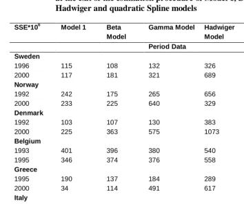
In cases of non-enhanced early-age fertility Model 1 and the Beta model provide the best fits for the majority of the cases examined. More analytically for Sweden, Denmark, Norway, Belgium, Greece and Italy, Model 1 provides the best fits among the Gamma, Hadwiger and quadratic Spline models. Considering the values of the minimization criterion at the exit of the estimation procedure, given in Table 11 we observe that Model 1 provides closer fits than the Beta model for most of the data sets although the later requires the estimation of more parameters. The quadratic Spline model provides quite reliable fits. In most cases, it provides better fits than the Gamma and the Hadwiger models. However in some cases such as the population of Sweden for the year 1996, the Spline model tends to underestimate the data above age 40. The Gamma and the Hadwiger model according to the values of the residual sum of squares (Table 11) provide the less successful fits among all the models examined. The only exception is the case of Belgium where the Gamma model gave the best fits for years prior to 1990.

A remarkable observation is that for some countries such as Norway and Sweden for years after 2000, the models mentioned above fail to adequately represent fertility at early ages, which implements the existence of enhanced early-age fertility. As it is demonstrated in the sequence, even for these countries, mixture models such as Model 2 and the Hadwiger Mixture model are required for fitting the single-year age-specific fertility distribution.

Coale-Trussell (1974) and the Gamma models perform equally well. On the contrary they have rejected the Beta model since it gave very disappointing results namelythe worst results among all the models they examined. However they have mentioned that the disappointing results obtained for the Beta density were due to the fact that the computer runs did not result in a real least-squares approximation of the beta density but only gave a local minimum. The authors argued that by refining the number of iterations the Beta model resulted in the better fits among all models tested apart from Splines. In our calculations the Beta model, as already mentioned, is among the models that provide very reliable fits in the majority of the cases. Furthermore it is worth mentioning that in the literature the parameters _α,_β have been interpreted as the lower and upper age limit of fertility. However in our results the values of the estimated parameter β has in many cases a value greater of 100, as shown in Tables 2 and 4, which of course cannot be interpreted as the upper age limit of fertility. Hoem et al. (1981) have also mentioned that in their applications the estimated value of β was 204 which demonstrates that the interpretation of this parameter as the upper age limit of fertility is untenable.

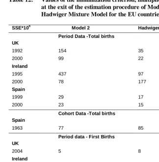
In a more thorough evaluation of the above results one can mark that for the year 2000, Denmark, Sweden, Norway and Italy show a slight hump at early-ages fertility rates. This new pattern of enhanced early-age fertility cannot be captured by the models that have previously been described. Therefore we also evaluate Model 2 and the Hadwiger Mixture model. These models provide an improved fit at the early ages of fertility. Mixture models are also used for fitting the age-specific fertility distributions of the UK, Ireland, Spain and the US. Generally the Hadwiger Mixture model and Model 2 provide equivalent successful fits to the empirical data. However in the case of the US, these models cannot provide adequate fits. Therefore we also evaluate the adjusted version of Model 2. This model provides very close fits of the US fertility schedules. The values of the minimization criterion are given in Tables 12 and 13. While a graphical illustration of the results is given in Figures 2 and 3 respectively.

Our findings imply that there is a strong evidence of heterogeneity in female populations. It should be exceptionally interesting to identify and describe the sources of heterogeneity in fertility. In the literature it has been stated that this heterogeneity in is closely related to teenage fertility most of it non-marital for the UK and Ireland (Chandola et al., 1999). It has been cited that apart from the UK and Ireland there are other European countries with high proportions of birth outside marriage such as Sweden and Denmark which do not show this hump at the early ages of the fertility curve. Chandola et al. (1999) mentioned that this may be explained for countries such as Sweden and Denmark, since these populations do not show big heterogeneity with respect to the timing and volume of non-marital fertility; they do not have the exceptionally high teenage fertility rates of the UK and Ireland and furthermore individuals or cohabiting couples producing births outside marriage are behaving demographically more like married couples. Moreover according to Chandola et al. (1999), in populations where the fertility distribution is fitted by a simple model the behaviour characterized by births outside marriage has been adopted by the mainstream of society in such a way that there is not much difference between the mother‘s characteristics for marital and non-marital births. While for populations requiring a mixture model, the adoption of extramarital fertility has made the society more heterogeneous in respect of fertility characteristics. However we observe from our empirical investigations that this distorted fertility distribution has arisen recently even for populations such as Denmark, Sweden and Norway and therefore an additional explanation of it is required. In the case of the US an important factor which may account for the marked heterogeneity is the difference in fertility between different or racial groups and in particular the differences in the timing of births between these groups (Chandola et al., 2002).

It isremarkable that the pattern of first births also exhibits a strongly intense hump at younger ages. This heterogeneity is also apparent in the US fertility schedules differentiated by ethnicity of the mother. Therefore the heterogeneity present in these countries might not only attributed to marital status, ethnic differences or birth order but other factors should be taken into account such as the educational, social and economical ones.

pattern is that the percentages of low educated young females that leave below the poverty level as well as of ‘solo’ mothers are high in the UK.

In Spain enhanced early-age fertility is also observed for first births, which implies a strong heterogeneity in female population. However given that out-of-wedlock childbearing is still relatively rare, pre-marital cohabitation is not wide-spread and there is a strong tendency with late home-leaving and late union-formation (Kohler et al., 2006; De Sandre, 2000; Delgado and Castro, 1998), heterogeneity in Spanish fertility should be associated to a great extent to the growth of immigrant populations from third-world origins with higher and earlier patterns of fertility compared with those of the indigenous populations. Religiosity may also contribute to the existence of a distorted fertility distribution in recent years in Spain. Adsera (2004) found that in Spain according to the 1985 Spanish Fertility Survey (SFS) family size was similar among practicing and non-practicing Catholics. A decade and a half later, according to the 1999 SFS, practicing Catholics portrayed significantly higher fertility than others. Furthermore the small group of conservative Protestants and Muslims has the highest fertility in Spain (Adsera, 2004).

InScandinavian countries, heterogeneity in fertility could also be associated to the second generation immigrants from Arabic and Eastern countries.

Finally in the case of the US an important factor which may account for the marked heterogeneity is the difference in fertility between racial groups and in particular the differences in the timing of births between these groups (Chandola et al., 2002). In general Black and Hispanic mothers begin childbearing earlier than do non-Hispanic whites and they have much higher proportions of births outside marriage. The fertility pattern for the white population is also heterogeneous. Chandola et al. (2002) stated that this is not only due to the growing proportion of births outside marriage but also due to substantial number of Hispanic births within the white group. However we consider that religion, as well as the educational and the social status of mothers may also be a source of heterogeneity in the US fertility distribution. In a recent study Frejka and Westoff (2006) state that religion play a more important role in the lives of Americans compared to Europeans. The only exceptions are Ireland and Italy, where religiosity is similar to that of the US.

6. Conclusions

Many models have been proposed for modeling fertility schedules but little interest is shown in fitting low-fertility schedules of modern populations. In addition a new distorted fertility pattern has arisen the recent years for many populations characterized by a bulge at early fertility ages. Most of the models existing are inadequate for describing this phenomenon.

In this work, three versions of a parametric model are proposed in order to describe the typical pattern as well as the new one. Model 1 describes the fertility pattern in populations that do not show high early age fertility while Model 2 and its adjusted version are useful for populations that show the new distorted fertility pattern. In order to evaluate the adequacy of the models proposed, we fit the three alternative formulae to a variety of period and cohort data sets of several populations. Furthermore we compare these with other models already existed. Finally in order to avoid heterogeneity we also fit the models to data differentiated by order of birth and, where such data were available, by race.

For both period and cohort data, Model 1 provides the best fits among the models considered for the majority of the cases while the Beta model performs equally well. Thus Model 1 proves superior since it includes fewer parameters than the Beta Model. For period data, the quadratic Spline model gave sufficient fits but it many cases it underestimated the ends of the fertility curve. In the case of cohort data the Spline proves less sufficient than the other models. The Hadwiger and the Gamma models provided the less successful fits for most of the data sets used, for both period and cohort data. The only exception is the case of period data for Belgium where the Gamma model gave the best fits for years prior to 1990.

Regarding Model 2 and its adjusted version, used for describing populations with enhanced early-age fertility, both provide successful fits of the distorted fertility schedules, equivalentto the ones provided by the Hadwiger Mixture model. Although both Model 2 and the Hadwiger Mixture model require the same number of parameters to be estimated, the model we propose is much simpler and easier to interpret. Its parameters have an explicit demographic interpretation. Whilr the estimated parameters can easily be utilized for understanding the shape of the fertility pattern and for comparisons through time, place, cohorts, population’s subgroups and order of births.

mainstream of society for countries with high proportion of non-marital births such as Denmark, Norway and Sweden. In the case of Spain a possible explanation that needs further research is that the population has been heterogeneous due to the growth of second generation immigrant populations from third-world origins with still higher and earlier patterns of fertility compared with those of the indigenous population. Other factors also may be associated to the strong heterogeneity present in Spain such as the educational level and the economic status as well as the religiosity of the mothers. Regarding Ireland the strong Catholicism may be associated with the heterogeneity in recent populations. In the case of the UK the great heterogeneity may be associated to the fact that there is a great majority of solo mothers as well as with the low educational level of mothers. Furthermore it becomes obvious that the US is characterized by a distinctive age-specific fertility pattern which implies a great heterogeneity in the female population.

Another finding is that for countries with enhanced early-age fertility the pattern of first births also exhibits a strongly intense hump in younger ages and even stronger than the pattern of total fertility. Furthermore the fertility pattern of the US when differentiated by the ethnicity of the mother is quite heterogeneous. This fact provides a strong evidence of heterogeneity in the female populations associated not only to the marital status, race and birth order but also to the educational level, social and economic status as well as the religiosity of the mothers.

7. Acknowledgements

References

Adsera, A. (2004). “Marital Fertility and Religion: Recent Changes in Spain”, Discussion paper, no 1399, IZA (Institute for the Study of Labor), Bonn.

Berge, E. (1974b). “Regionale variasjonar i fertiliteten i Norge omkring 1970.” Central Bureau of Statistics of Norway, Working Paper IO 74/40.

Bongaarts, J. and Feeney, G. (1998). “On the Quantum and Tempo of Fertility.”,

Population and Development Review, 24: 271-292.

Brass, W. (1960). “The graduation of fertility distributions by polynomial functions.”,

Population Studies, 14: 148-162.

Brass, W. (1974). “Perspectives in Population Prediction: Illustrated by the Statistics of England and Wales (with discussion).”, Journal of the Royal Statistical Society

A, 137: 532-583.

Brass, W. (1978). Population Projections for Planning and Policy. Papers of the East-West Population Institute, No 55. Honolulu, Hawaii.

Chandola. T., Coleman, D. A., Horns, R. W. (1999). Recent European fertility patterns: fitting curves to ‘distorted’ distributions. Population Studies, 53, 3: 317-329.

Chandola. T., Coleman, D. A., Horns, R. W. (2002). Distinctive features of age-specific fertility profiles in the English-speaking world: Common patterns in Australia, Canada, New Zealand and the United States, 1970-98. Population Studies, 56, 181-200.

Coale, A.J. and Trussell, T. J. (1974). “Model fertility schedules: variations in the age structure of childbearing in human populations.”, Population Index, 40, 2: 185-258

Coale, A.J. and Trussell, T. J. (1978). “Technical note: finding the two parameters that specify a model schedule of marital fertility.” Population Index, 44, 2: 203-214.

Delgado, M. and T. Castro Martin (1998). Fertility and Family Surveys in Countries of the ECE Region, Standard Country Report Spain. Geneva: United Nations.

De Sandre, P. (2000). “Patterns of Fertility in Italy and factors of its Decline.”, Genus, 56, 1-2: 19-54.

Farid, S. M. (1973). “On the pattern of cohort fertility.”, Population Studies, 27: 159-168.

Frejka, T. and Westoff, C. F. (2006). “Religion, Religiousness and Fertility in the U. S. and Europe.”, MPIDR Working Paper WP 2006-013, May 2006.

Gilks, W. R. (1986). “The relationship between birth history and current fertility in developing countries.”, Population Studies, 40.

Gilje, E. (1969). Fitting curves to age-specific fertility rates: some examples. Statistical Review of the Swedish National Central Bureau of Statistics III, 7:118-134.

Hadwiger, H. (1940). “Eine analytische reprodutions-funktion fur biologische Gesamtheiten.”, Skandinavisk Aktuarietidskrift, 23, 101-113.

Hoem, J. M. (1976). “The statistical theory of demographic rates: A review of current developments (with discussion).”, Scandinavian Journal of Statistics, 3: 169-185.

Hoem, J. M., Madsen, D., Nielsen, J. L., Ohlsen, E., Hansen, H. O., Rennermalm, B. (1981). “Experiments in modelling recent Danish fertility curves.”,

Demography, 18: 231-244.

Hoem, J. M. and Rennermalm, B. (1978). “On the statistical theory of graduation by Splines,”, University of Copenhagen, Laboratory of Actuarial Mathematics. Working Paper No. 14.

Karlis, D. and Kostaki, A. (2002). “Bootstrap techniques for mortality models.”,

Biometrical Journal, 44, 7: 850-866.

Kohler, H-P., Billari, F. C. and Ortega, j. A. (2006). “Low Fertility in Europe: Causes, Implications and Policy Options. In F.R. Harris(Ed.), The Baby Bust: Who will do the Work? Who Will Pay the Taxes?”, Lanham, MD: Rowman & Littlefield Publishers, 48-109.

Kohler, H-P, Philipov, D. (2001). “Variance effects in the Bongaarts-Feeney formula.”,

Demography, 38, 1: 1-16.

Kohler, H-P., Ortega, J. A. (2002). “Tempo-adjusted period parity progression measures, fertility, postponement and completed cohort fertility.”, Demographic

Research, 6, 6: 91-144.

http://www.demographic-research.org/Volumes/Vol6/6-6.pdf.

Murphy, E. M. and Nagnur, D.N. (1972). “A Gompertz fit that fits: Applications to Canadian Fertility Patterns.” Demography, 9: 35-50.

Nurul Islam, M. and Mallick S. A. (1987). “On the use of a truncated Pearsonian Type III curve in fertility estimation.”, Djaka University Studies, Part B Science, 35, 1: 23-32.

Romaniuk, A. (1973). “A three parameter model for birth projections.”, Population

Studies, 27, 3: 467-478.

Ryder, N. B. (1964). “The process of demographic translation.”, Demography, 1,1: 74-82.

Ryder, N.B. (1980). Components of temporal variations in American fertility. In R.W. Hiorns (ed.), Demographic patterns in developed societies. Symposia of the Society for the Study of Human Biology, Vol XIX, Taylor and Francis Ltd., London, 15-54.

Schmertmann, C. P. (2003). “A system of model fertility schedules with graphically intuitive parameters.”, Demographic Research, 9,5:82-110.

US National Centre of Health Statistics:

http://www.cdc.gov/nchs/datawh/statab/unpubd/natality/.

Yntema, L. (1969). “On Hadwiger‘s fertility function.”, Statistical Review of the Swedish National Central Bureau of Statistics III, 7, 113-117.

Appendix A

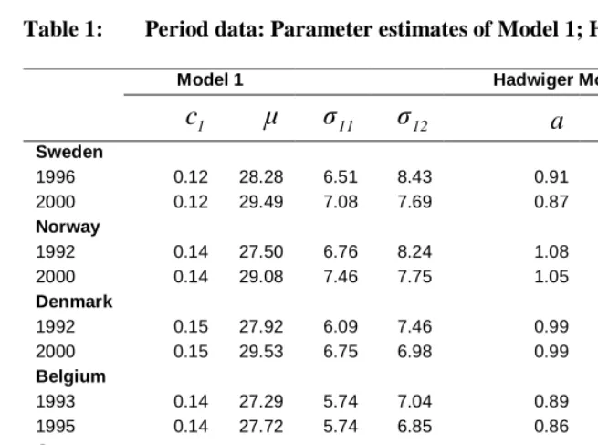
Table 1: Period data: Parameter estimates of Model 1; Hadwiger Model

Model 1 Hadwiger Model

1

c

µ

σ

σ

_a

_b

_c

Sweden

1996 0.12 28.28 6.51 8.43 0.91 3.85 29.78 2000 0.12 29.49 7.08 7.69 0.87 3.99 30.44

Norway

1992 0.14 27.50 6.76 8.24 1.08 3.69 28.86 2000 0.14 29.08 7.46 7.75 1.05 3.79 29.95

Denmark

1992 0.15 27.92 6.09 7.46 0.99 4.16 29.09 2000 0.15 29.53 6.75 6.98 0.99 4.30 30.25

Belgium

1993 0.14 27.29 5.74 7.04 0.89 4.31 28.39 1995 0.14 27.72 5.74 6.85 0.86 4.44 28.71

Greece

1995 0.09 27.08 6.71 8.37 0.75 3.63 28.53 2000 0.09 28.98 7.87 7.72 0.72 3.66 29.73

Italy

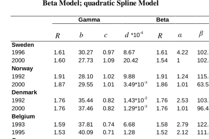
Table 2: Period data: Parameter estimates of Gamma Model; Beta Model; quadratic Spline Model

Gamma Beta

R b c d*10-4 R α β ν τ2

Sweden

1996 1.61 30.27 0.97 8.67 1.61 4.22 102.75 16.77 48.81 2000 1.60 27.73 1.09 20.42 1.54 1 102.59 22.12 55.32

Norway

1992 1.91 28.10 1.02 9.88 1.91 1.24 115.57 19.88 63.63 2000 1.87 29.55 1.01 3.49*10-3 1.86 1.01 63.576 15.33 18.59

Denmark

1992 1.76 35.44 0.82 1.43*10-2 1.76 2.53 103.76 22.02 62.99 2000 1.76 37.46 0.82 1.29*10-3 1.76 1.01 96.481 24.52 56.59

Belgium

1993 1.59 37.81 0.74 6.68 1.58 2.79 122.12 24.39 90.59 1995 1.53 40.09 0.71 1.28 1.52 2.12 111.51 26.28 83.03

Greece

1995 1.32 27.21 1.04 6.1 1.32 1.78 134.15 19.24 77.41 2000 1.27 27.41 1.07 4.2 *10-3 1.27 1.01 91.435 18.17 40.07

Italy

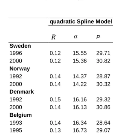
Table 2: (Continued)

quadratic Spline Model

R α P H

Sweden

1996 0.12 15.55 29.71 35.56 2000 0.12 15.36 30.82 36.17

Norway

1992 0.14 14.37 28.87 34.61 2000 0.14 14.22 30.32 35.77

Denmark

1992 0.15 16.16 29.32 34.49 2000 0.14 16.13 30.86 35.71

Belgium

1993 0.14 16.34 28.64 33.54 1995 0.13 16.73 29.07 33.82

Greece

1995 0.09 14.16 28.37 34.28 2000 0.09 13.27 30.15 35.64

Italy

Table 3: Cohort data: Parameter estimates of Model 1; Hadwiger Model

Model 1 Hadwiger Model

1

c

µ

σ

σ

a

b

c

Spain

1942 0.22226 25.45 4.5792 9.3192 1.5497 3.8729 28 1963 0.10801 28.823 9.0866 7.7493 0.90669 3.3022 29.23

Table 4: Cohort data: Parameter estimates of Gamma Model; Beta Model; quadratic Spline Model

Gamma Model Beta Model

R

b

c

d

R

α

β

ν

τ

Spain

1942 2.75 10.001 1.62 11.89 2.74 14.63 371.14 6.61 166.04 1963 1.67 21.93 1.38 0.004 1.59 1.002 49.82 9.49 7.59

quadratic Spline Model

R

α

Spain

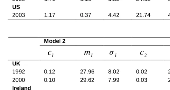
Table 5: Period data: Parameter estimates of Hadwiger Mixture Model and Model 2

Hadwiger Mixture Model

R

a

b

c

d

e

UK

1992 1.06 1.45 2.41 32.62 4.36 40.89 2000 0.94 0.29 4.64 21.88 4.59 31.40

Ireland

1995 1.05 0.15 5.16 21.85 4.74 31.84 2000 1.09 0.23 4.41 22.84 5.19 32.83

Spain

1999 0.68 0.19 3.67 24.26 5.59 32.29 2000 0.71 0.19 3.82 24.01 5.61 32.38

US

2003 1.17 0.37 4.42 21.74 4.37 30.81

Model 2

1

c

m

σ

c

m

σ

UK

1992 0.12 27.96 8.02 0.02 20.00 2.42 2000 0.10 29.62 7.99 0.03 20.27 3.23

Ireland

1995 0.13 30.83 7.28 0.02 20.21 2.74 2000 0.14 31.76 6.97 0.04 20.77 3.43

Spain

1999 0.01 20.37 3.41 0.1 31.38 6.26 2000 0.02 20.57 3.49 0.1 31.50 6.28

US

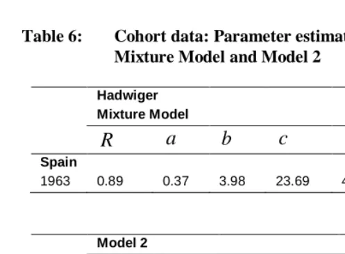
Table 6: Cohort data: Parameter estimates of Hadwiger Mixture Model and Model 2

Hadwiger Mixture Model

R

a

b

c

d

e

Spain

1963 0.89 0.37 3.98 23.69 4.90 31.16

Model 2

1

c

m

σ

c

m

σ

Spain

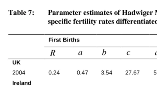
Table 7: Parameter estimates of Hadwiger Mixture Model in age- specific fertility rates differentiated by birth order

First Births

R

a

b

c

d

e

UK

2004 0.24 0.47 3.54 27.67 5.67 31.40

Ireland

2000 0.43 0.32 5.66 21.10 5.45 30.62

US

2003 0.05 0.73 3.25 23.53 5.54 32.21

Second Births

R

a

b

c

d

e

UK

2004 0.20 0.59 3.93 29.52 7.21 33.76

Ireland

2000 0.33 0.39 3.81 27.40 6.29 33.05

US

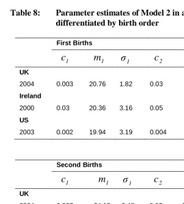
Table 8: Parameter estimates ofModel 2 in age-specific fertility rates differentiated by birth order

First Births

1

c

m

σ

c

m

σ

UK

2004 0.003 20.76 1.82 0.03 29.76 6.72

Ireland

2000 0.03 20.36 3.16 0.05 29.79 6.12

US

2003 0.002 19.94 3.19 0.004 26.88 8.64

Second Births

1

c

m

σ

c

m

σ

UK

2004 0.007 24.13 3.48 0.03 32.18 6.004

Ireland

2000 0.009 22.57 3.31 0.05 31.72 6.13

US

Table 9: Parameter estimates of Model 2 and Hadwiger Mixture Model for the US (2003), differentiated by origin

Model 2

US 2003

_c

σ

c

m

σ

White

0.04 20.31 3.19 0.12 28.31 8.45

Black

0.079 20.45 3.9 0.09 27.27 9.14

Indian

0.06 20.49 3.92 0.08 26.89 8.61

Asian

0.02 20.03 2.82 0.13 29.95 8.02

Hadwiger Mixture Model

US 2003

_R

a

_b

c

_d

e

White

1.18 0.35 4.48 21.82 4.41 30.76

Black

1.14 0.43 4.63 20.83 3.67 29.71

Indian

0.96 0.25 5.35 20.01 3.29 27.77

Asian

Table 10: Parameter estimates of Adjusted Model 2 for the US (2003), differentiated by origin and birth order

Adjusted Model 2

US 2003

c

m

11

σ

σ

c

m

σ

Total Births

0.086 20.27 3.45 10.26 0.08 30.61 7.42

First Births

0.003 19.31 2.58 4.69 0.0041 27.33 8.54

Second Births

0.03 21.28 2.98 5.52 0.04 30.2 6.95

White Births

0.08 20.23 3.31 10.01 0.09 30.34 7.46

Black Births

0.13 20.22 3.71 11.03 0.03 33.29 6.64

Asian Births

0.03 20.19 3.19 11.14 0.11 30.66 7.53

Indian Births

Table 11: Values of the minimization criterion multiplied by 100.000, at the exit of the estimation procedure of Model 1, Beta, Gamma, Hadwiger and quadratic Spline models

SSE*106 Model 1 Beta Model

Gamma Model Hadwiger Model

quadratic Spline Model Period Data

Sweden

1996 115 108 132 326 174

2000 117 181 321 689 174

Norway

1992 242 175 265 656 263

2000 233 225 640 329 287

Denmark

1992 103 107 130 383 169

2000 225 363 575 1073 287

Belgium

1993 401 396 380 540 462

1995 346 374 376 558 525

Greece

1995 190 137 184 289 101

2000 34 114 491 617 55

Italy

1995 20 58 139 352 49

2000 47 71 524 908 82

Cohort Data Spain

1943 732 1005 1159 1547 5450

Table 12: Values of the minimization criterion, multiplied by 100.000, at the exit of the estimation procedure of Model 2 and Hadwiger Mixture Model for the EU countries

SSE*106 Model 2 Hadwiger Mixture Model Period Data -Total births

UK

1992 154 35

2000 99 22

Ireland

1995 437 97

2000 78 177

Spain

1999 29 17

2000 23 15

Cohort Data -Total births Spain

1963 77 85

Period data - First Births UK

2004 5 8

Ireland

2000 73 53

Period data - Second Births UK

2004 4 5

Ireland

Table 13: Values of the minimization criterion, multiplied by 100.000, at the exit of the estimation procedure of Adjusted Model 2, Hadwiger Mixture Model and Model 2 for the US data

SSE*106 Adjusted Model 2 Hadwiger Mixture Model 2

US 2003

Total Births 150 28 1874 First Births 0.086 4 0.6 Second Births 3.5 348 25

White 28 156 728

Black 39 190 485

Asian 61 148 69

APPENDIX B