Volume 8 - Article 2 | Pages 31–60

of peer-reviewed research and commentary in the population sciences published by the Max Planck Institute for Demographic Research Konrad-Zuse Str. 1, D-18057 Rostock · GERMANY www.demographic-research.org

DEMOGRAPHIC RESEARCH

VOLUME 8, ARTICLE 2, PAGES 31-60

PUBLISHED 22 January 2003

www.demographic-research.org/Volumes/Vol8/2/

DOI: 10.4054/DemRes.2003.8.2

Research Article

On Monotonic Convergence to Stability

Dalkhat Ediev

1 Introduction 32

2 The population projection model 33

3 The Kullback information distance as a member of a wider class of distances

35

4 Proof of monotonic convergence to stability 37 5 Examples of monotonic measures and numerical

results

38

6 Populations monotonically converge to each other when they follow similar reproduction regimes

42 6.1 Two populations with similar time-independent

reproduction rates (convergence under the strong ergodicity conditions)

42

6.2 Two populations following similar time-dependent reproduction regimes (convergence under the weak ergodicity conditions)

44

7 Are there other classes of monotonic measures? 45

8 Applications 46

9 Acknowledgements 54

References 55

Appendix. Numerical results for illustrative examples presented in the text

Research Article

On Monotonic Convergence to Stability

Dalkhat Ediev1

Abstract

The paper introduces, for age-distribution population vectors, a class of distances to the stable equivalent; each of these distances converges monotonically to zero as the population approaches stability. The Kullback distance, considered earlier to be unique as a measure with this property, turns out to be a mere specimen of this class. It is shown that the very feature of monotonic convergence agrees with demographic potential of age specific stabilization measures. The paper also introduces a class of monotonic measures of the convergence to each other of two non-stable populations with similar reproduction regimes. Numerical illustrations and demographic applications conclude the paper.

1. Introduction

Monotonic measures for convergence of the population to its stable equivalent were imported into demography from the thermodynamic concept of entropy and from the information theoretical concept of informational distance. This paper contributes to the subject by widening the class of such monotonic measures. Firstly, we consider the classical population projection model with constant rates and suggest the class of monotonic measures for stabilization. These measures are weighted sums of age-specific deviations from the stable equivalent population, including as a special case the Kullback distance investigated in the literature. Next, we turn to the convergence to each other of two non-stable populations with similar reproduction regimes and show that monotonic measures for convergence of such populations form a subclass of the aforementioned monotonic measures. Finally, we explore the convergence in the case of time-dependent reproduction regimes and suggest monotonic measures for convergence in that case. Being weightening factors, demographic potentials play an important role in the monotonic measures proposed. Discrete one-sex models closed to migration are considered throughout the paper, but continuous analogs are straightforward. Results of the work are accompanied by numerical illustrations and are applied to explore the convergence of racial groups of the US population.

In his paper “Why use population entropy? It determines the rate of convergence” Tuljapurkar (1982) introduced the informational distance as a monotonic measure of convergence of age structure to the stable equivalent. Later Schoen and Kim (1991) developed this idea and argued that the Kullback information distance is suitable for demographic needs and it can reflect instantaneous movements towards the stable equivalent. It was recently proved that monotonic convergence to stability by the Kullback distance is equivalent to the ergodic property for linear population models with nonnegative reproduction rates [Ediev 2002a]. These results leave the impression that the Kullback distance is particularly suitable for age-structured models and represent some important features of demographic systems. Schoen and Kim, for example, wrote:

“… the only other [besides the Kullback distance – D.E.] monotonic measure of which we are aware is described in Golubitsky, Keeler, and Rothschild (1975). That measure is less appealing than the Kullback distance because it assures monotonicity only in the maximum deviation of observed age-specific values from their stable counterparts” [Schoen and Kim 1991: 465].

When the paper was being reviewed, the author found another work on the monotonic measures of convergence to stability. Independently from the aforementioned works Rubinov and Chistyakova developed the quantity called ‘the indicator of instability’ [Rubinov and Chistyakova 1986: 50, 51]. They corrected the measure proposed by Pirozhkov (1976) and pointed to the monotonicity as an important unique feature of the indicator they developed.

In fact both the Kullback distance and the Pirozhkov-Rubinov-Chistyakova’s index of instability turn out to be a mere specimens of the class proposed in the paper.

2. The population projection model

In this section we rewrite the classical population projection model in a form more convenient for the purposes of the paper. The form we propose arises from the model of reproduction based on the concept of demographic potential [Ediev 2000, 2001a: 325-329, 2001b, 2001c] but it is fully equivalent to the classical component model as well. In the cohort-component model [Leslie 1945], age-specific mortality and fertility rates are used to model the dynamics of the population age structure. In that model, the dynamics of the youngest age group is described by the following difference equation:

( )

∑

(

)

=

−

=

+

X

x

x x

F

L

x

t

n

t

n

0 0

0

1

, {1}

where nx

( )

t is the size of age group

x

at time

t

, Lx is the accumulated probability of surviving from age

0

to age

x

, and F_x is the age-specific fertility rate corrected for

infant mortality (

x

=

0

,

1

,

2

,...,

X

) .

Fisher’s reproductive value v_x of a person of age

x

[Fisher 1930] is the net present value of future births of that person discounted by the intrinsic rate of population increase. In the discrete case [Leslie 1948] it can be written as:

( )

∑

=

− + −

=

X

x y

x y y x y

x

F

L

L

v

λ

1 , {2}

1 +

−

=

_{x x x}

x

v

P

v

F

λ

, {3}

where

P

_x is the probability of surviving from age

x

to age

x

+

1

. Using {3}, the difference equation {1} can be rewritten in the form:

∑

= −

+

=

∆

X

x x t x

t

b

b

0

1 , {4}

where

( )

t t

t

n

b

λ

0

=

is the discounted number of births at time

t

;

∆

=

_x

−

_x+1

def

x

u

u

;

and

x x x x

L

v

u

λ

=

is the expected relative future demographic potential at age

x

for

today’s newborn [Ediev 1999], for the population with time-constant fertility and mortality rates it simply equals to the expected present value of the reproductive value to be attained by a newborn at age

x

. The concept of demographic potential is close to the reproductive value in the sense that it measures the relative contribution of persons from different population groups to the ultimate population size. Unlike the reproductive values, which correlate contributions of contemporarily living persons, the demographic potentials measure relative contributions of persons at arbitrary ages, from arbitrary birth cohorts, taken at arbitrary time periods. In addition, the demographic potential concept can be extended to the case of time-dependent reproduction regimes.

The total reproductive value of the population can be rewritten in the new notation as:

( )

∑

( )

∑

= −

=

=

=

X

x

x t x t X

x x

x

n

t

u

b

v

t

V

0 0

λ

{5}

Under the ergodic property [Arthur 1981, 1982], discounted births tend to a constant level determined by the stable equivalent [Keyfitz 1969], as

t

tends to infinity:

( )

0

* 0 *

n

b

b

def

t

→

=

as

t

→

∞

Combining this with {5} and taking into account the exponential dynamics of the total reproductive value [Fisher 1930] we have:

( )

( )

U

V

U

t

V

b

* _t

=

0

⋅

=

λ

, {6}

where

∑

=

=

X

x x

u

U

0

.

3. The Kullback information distance as a member of a wider class

of distances

The Kullback-Leibler distance [Kullback and Leibler 1951, Kullback 1959] measures

the dissimilarity between two vectors (

y

, y

*) containing components of some probability distributions:

∑

=

















=

X

x _x

x x

y

y

y

K

0 *

ln

, {7}

where the quantities y_x are non-negative and sum to one, and similarly for the

quantities y .*_x

As proposed by Tuljapurkar (1982), the age distribution of reproductive values could be substituted into {7} in order to get a monotonic measure of convergence to stability. In our notation this distribution is given by the following expression:

( )

( )

(

)

( )

0

( )

0

0 0

0

V

u

b

V

L

L

u

L

L

x

t

n

t

V

v

t

n

y

_t x t x x

x x x

x x t

x

=

−

−

=

=

λ

λ

{8}

Substituting by {6}, we have for the stable equivalent population:

( )

U

u

V

u

b

y

_x

=

x

=

x

0

*

Combining {7}-{9}, we finally get the following expression for the Kullback distance:

∑

∑

= − − =













=

















=

X x x t x t x X x _x t x t x t

b

b

b

b

u

U

y

y

y

K

0 * *

0 *

ln

1

ln

{10}

As it was shown by Tuljapurkar (1982), this distance converges monotonically to zero as the population approaches stability. The quantity Kt in {10} is a ‘one-way’ distance from the population structure at moment

t

to the structure of the stable equivalent. As it is shown in [Ediev 2002a], monotonic convergence to stability can be observed in two other information distances, one which measures the ‘one-way’ distance in the opposite direction, i.e. from the stable equivalent to the current population structure, and the symmetrical distance defined as the average of the two others:

∑

∑

= − =

















=

















=

X

x t x

x X

x t_x

x x t

b

b

u

U

y

y

y

K

0 * 0 *

*

_ln

1

_ln

w

{11}

(

)

∑

∑

= − − =

























₋

=

















−

=

+

=

X x x t x t x X x _x t x x t x t t t

b

b

b

b

u

U

y

y

y

y

K

K

K

0 * *

0 *

*

₁

_ln

2

1

ln

2

1

2

ˆ

w

{12}

From {10}-{12} it follows that all three variants of the information distance can be treated as measures of the following type:

(

)

∑

= −

=

X

x x t x

t

u

d

b

b

D

0

*

;

, {13}

where

(

*

)

; b

b

d _t−x is a function which measures one-dimensional deviation of bt−x from its stable equivalent b . The purpose of this paper is to prove that under* unrestrictive assumptions about the deviation function

( )

*

; b b

d , viz that is a convex

function of

b

and satisfies

d

( )

b

;

b

=

0

for all

b

, every measure of the form {13} converges monotonically to 0 for increasing

t

, that is, as the population approaches stability. Convexity condition is granted if, for example, the second derivative

( )

* 2 2 ;b b d b ∂

4. Proof of monotonic convergence to stability

The following expression can be obtained for changes in distance {13}:

(

)

(

) (

*

)

1 0 1

0

* 1

0

*

1

u

d

b

;

b

u

d

b

;

b

u

d

b

;

b

D

D

_t

X

x x t x

X

x x t x

t

t +

−

= + −

= −

+

=

−

−

−

∑

∑

{14}

By rearranging, by using {4}, and taking into account that u₀ =1 and u_X+1=0, we get:

(

)











 ∆

−

∆

=

−

_∑

_∑

= −

= −

+ *

0 0

*

1

d

b

;

b

d

b

;

b

D

D

X

x x t x X

x x t x

t

t {15}

Indeed, the reproduction coefficients ∆_x should be nonnegative for monotonic convergence in the Kullback distance, as shown in [Ediev 2002a]. This condition is assured for the cohort-component model, as fertility rates are necessarily nonnegative. We also assume this condition to be met, i.e. ∆x≥0,x=0,X. Then monotonic

convergence of distance {13} is simply a consequence of the Jensen’s inequality for convex functions [Hardy, Littlewood, and Polya 1934]:

( )













≥

∑

∑

k k k

k k k

x

a

f

x

f

a

{16}

for any convex function

f

( )

x

if

a

_k

≥

0

and

∑

=

1

k k

a

. We should only note that

1

0 0

=

=

∆

∑

=

u

X

x x

to obtain the following result from the Jensen’s inequality, the convexity assumption imposed on the deviation function, and expression {15}:

0

1

≥

−

_t+

t

D

D

, i.e.

D

_t+1

≤

D

_t for any

t

{17}

Assume that the ergodic property holds for the reproduction model {1}, {4}. Indeed, as proved in [Ediev 2002a], this is the necessary and sufficient condition for monotonic convergence in the Kullback distance for models with a nonnegative projection matrix. Then it follows from the condition

d

( )

b

;

b

=

0

imposed on the deviation function and from the continuity of that function (this property is granted for any convex function defined on the set of all real numbers [e.g. Polyak 1983: 118]), that distance {13} tends to zero as the population structure approaches the structure of the stable equivalent and

t

b

approaches * b .

5. Examples of monotonic measures and numerical results

The results obtained suggest that different distances can be constructed, which decrease to zero monotonically as time goes on and the population approaches stability. In terms of population structures, these distances have the following form:

( )

∑

= − − −

















=

X

x t x _x

x x x t x x x x t

L

n

L

t

n

d

v

L

D

0 *

;

λ

λ

λ

, {18}

where

d

( )

b

;b

* is a convex function of

b

and

d

( )

b

;

b

*

=

0

for

b

=

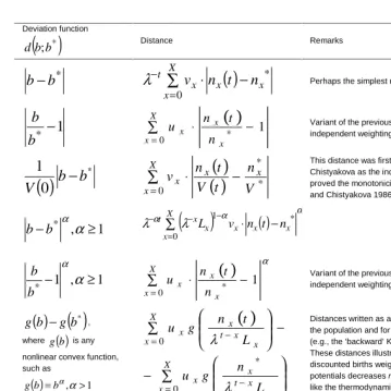
b

*. Table 5.1 presents some examples of such monotonic measures.

Table 5.1: Selected examples of monotonic measures of stabilization

Deviation function

( )

*

;b

b

d Distance Remarks

      * *ln b b Ub

b

( )

( )

∑

=         X x _x x x x x n t n n t n u

U 0 * *

ln 1

The Kullback distance {10}

        b b U * ln 1

( )

∑

=         X x x x x t n n u U 0 * ln 1

The Kullback distance in ‘backward’ direction {11}

            ₋ * * 1 ln

2 1 b b b b U

( )

( )

∑

=                 − X x _x x x x x n t n n t n u

U 0 * *

ln 1 2

1

Deviation function

( )

*

;b

b

d Distance Remarks

*

b

b

−

∑

( )

=

− X

_⋅

₋

x x x x

t

n

t

n

v

0 *

λ

Perhaps the simplest monotonic distance

1

*

−

b

b

( )

∑ = ⋅ − X x _x x x n t n u 0 *

1 Variant of the previous distance with time-_{independent weighting coefficients}

( )

0

*

1

b

b

V

−

( )

( )

∑

= ⋅ − X x x x x V n t V t n v 0 *

* This distance was firstly proposed by Rubinov and

Chistyakova as the indicator of instability. They also proved the monotonicity of this indicator [Rubinov and Chistyakova 1986: 50, 51]

1 ,

* _≥

−b α

α

b

( )

( )

α α α _λ λ ∑ = − −

− X _{⋅ −}

x x x x x x

t _{L v n t n} 0 * 1 1 , 1 * − α≥ α b

b

( )

∑ = ⋅ − X x _x x x n t n u 0 * 1 α

Variant of the previous distance with time-independent weighting coefficients

( )

_{b g}

( )

_b*

g − , where _g

( )

_b is any nonlinear convex function, such as

( )b =bα,α>1 g

( )

∑ ∑ = − = −         − −         X

x t x _x

x x

X

x t x _x

x x L n g u L t n g u 0 * 0 λ λ

Distances written as a difference between indexes for the population and for its stable equivalent separately (e.g., the ‘backward’ Kullback distance.)

These distances illustrate that any convex function of discounted births weighted by demographic potentials decreases monotonically, i.e., it behaves like the thermodynamic entropy with inversed sign

b b b b + − * *

( )

( )

∑

=

+

−

⋅

X

x _{x x}

x x x

t

n

n

t

n

n

u

0 * * 1 * * − − b b b e ( ) ∑ = −           − ⋅ X x n n t n x x x x e u 0 1 * *

Like the Kullback distance and the measures of the previous type, these distances are constructed of (not necessarily positive) deviation functions

Table 5.1 by no way comprehends all the possible monotonic measures. For example, monotonic distances can be based on the deviation function

where

d

( )

b

;b

* is any other deviation function and parameter

a

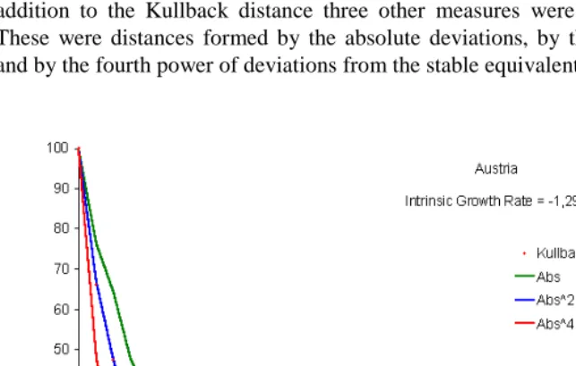
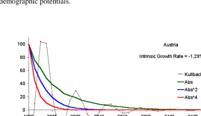
determines the threshold under which population differences are considered negligible (e.g. fluctuations). Other examples can also be suggested.

Hence, we have suggested a wide variety of distances which all exhibit monotonic convergence to zero as the stabilization goes on. The Kullback distance turns out to be a member of this class, being neither the only one nor the simplest. The following example illustrates how the different measures proposed above converge to zero. The age structure of the 1985 population of Austria [Keyfitz and Flieger 1990: 404-405] was projected till 2185 using the 1985 vital rates and zero migration assumptions. Values of monotonic measures were calculated for all years of the projection period. In addition to the Kullback distance three other measures were taken for the analysis. These were distances formed by the absolute deviations, by the quadratic deviations, and by the fourth power of deviations from the stable equivalent.

Figure 1 presents results of the calculations (‘Kullback’ stands for the Kullback distance; ‘Abs’ stands for the weighted sum of age-specific absolute deviations from the stable equivalent; ‘Abs^2’ stands for the weighted sum of quadratic deviations; and ‘Abs^4’ stands for the weighted sum of deviations in the 4th power.) Percents of initial distances to the stable equivalent are plotted for the sake of comparability. More detailed results are presented in table A1 of the Appendix.

It is seen that the distance formed by deviations in the fourth power has a steeper decline while the absolute deviations result in the slowest decline. More generally, the

higher the power

α

in the deviation function

α

1

*

−

b

b

, the steeper decline of the

stabilization measure. The absolute deviation forms the slowest stabilization measure since it is the only deviation function, which being a convex function, is also a concave function for negative and positive values of its argument. The Kullback distance behaves very close to the quadratic distance. This is natural since it can be approximated by the following quadratic expression when the population structure is close to stability:

=













₋

≈













_∑

∑

− − − − x x t x t x x x t x t x

b

b

Ub

b

u

b

b

Ub

b

u

ln

1

* * * *

∑

∑

∑













₋

=













₋

+













₋

=

− − − x x t x x x t x x x t x

b

b

u

U

b

b

u

U

b

b

u

U

2 * * 2 *

1

1

1

1

1

1

, {19}

where the latter equation follows from {5} and {6}.

quadratic nature of this measure itself rather than a reflection of the stabilization process. Another consideration important for practical applications is that the Kullback distance is highly sensitive to the age pattern of demographic potentials while other measures presented above are robust. This aspect will be illustrated in section 8 where possible demographic applications of monotonic measures will be discussed (figure 3.) Finally, we will see that it is the distance formed of absolute deviations, which monotonically reflects the convergence of age structures of two non-stable populations with similar time-dependent reproduction rates.

6. Populations monotonically converge to each other when they

follow similar reproduction regimes

6.1 Two populations with similar time-independent reproduction rates (convergence under the strong ergodicity conditions)

It follows from the results of Schoen and Kim (1991) as well as from the results presented above, that the rate of convergence to stability varies with time and depends on the population age structure. It would therefore be natural to expect that the dynamics of the distance between two arbitrary populations could not be monotonic, despite similar asymptotes. In spite of this, monotonic convergence of such populations can be granted, as demonstrated below. No doubt the monotonicity depends on particular characteristics of the measure used to reflect the distance between population structures. The Kullback distance, for example, fails to be a monotonic measure of population convergence. But there are other distances formed as a weighted sum of convex deviation functions, which do fit appropriate monotonicity conditions.

Let us consider the following distance between two population structures:

(

)

∑

= − −

=

X

x x t x t x

t

u

d

b

b

D

0

2

1

_;

_{, {20}}

where

b

_t1 and

b

_t2 are the discounted births of the two populations under consideration. Assuming that the same reproduction model {4} applies to both populations, we get:

(

;

)

;

0

0 2

0 1

0

2 1

1



≥











_∆

_∆

−

∆

=

−

∑

∑

∑

= −

= −

= − −

+

X

x

x t x X

x

x t x X

x

x t x t x t

t

D

d

b

b

d

b

b

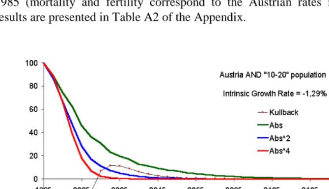
when the deviation function is a convex function of both of its variables. This means the monotonic convergence of {20} to zero under the conditions of ergodicity. The ‘reciprocal’ convexity of the deviation function is essential; both ‘one-way’ Kullback distances, for example, are convex functions of the first variable only. This explains why the Kullback distance between two non-stable populations does not converge to zero monotonically, while monotonicity is granted for symmetrical deviation functions. One example, though artificial, is presented in Figure 2, which reflects distances between the projected population of Austria and the population of people aged 10-20 in 1985 (mortality and fertility correspond to the Austrian rates in 1985). Numerical results are presented in Table A2 of the Appendix.

6.2 Two populations following similar time-dependent reproduction regimes (convergence under the weak ergodicity conditions)

This section investigates the question of monotonicity in the case of a time-dependent reproduction model, when only the weak ergodic property can be granted [Arthur 1982].

Let us start with additional notations for time-dependent demographic parameters. We denote by

L

_x

( )

t

the accumulated probability to survive from age

0

to age

x

for individuals born at time

t

. For time-dependent reproduction models it is convenient to use demographic potentials, which also depend on time, and no more relate to Fisher’s reproductive value [Ediev 1999]. We denote by

c

_x

( )

t

the demographic potential of a person aged

x

who was born at time

t

. The total demographic potential of the population turns out to be constant over time [Ediev 1999]. Using this property, we get the following model of reproduction:

(

)

∑

= −

+

=

∆

−

X

x x t x

t

t

x

b

b

0

1 {22}

where b_t = n₀

( ) ( )

t c₀ t is the total demographic potential of newborns at time

t

,

( )

t ux

( )

t ux

( )

t

x = − +1

∆ , and _{( )} ( ) ( )

( )t c

t L t c t

ux x x

0

= is the expected relative future

demographic potential at age

x

for newborn at time

t

. Again, we suppose that

( )

t

x

X

x

≥

0

,

=

0

,

∆

.

Following the same strategy as earlier, let us consider the following distance between two population structures:

(

)

(

)

∑

=

−

− −

=

X

x x t x t x

t

u

t

x

d

b

b

D

0

2

1

_;

_{23}

where

b

1_t

,

b

_t2 are the demographic potentials of newborns of the populations under consideration. Under reproduction model {22} applied to both populations, we get:

( )

(

;

)

( )

;

( )

0

0

2 0

1 0

2 1

1



≥











_∆

₋

_∆

₋

−

−

∆

=

−

∑

∑

∑

= −

= −

= − −

+

X

x x t x

X

x x t x

X

x x t x t x

t

t

D

t

x

d

b

b

d

t

x

b

t

x

b

when the deviation

d

( )

b

_t1

;

b

_t2 is a convex and homogeneous function of both its variables (e.g.

b

−

b

* ). This implies monotonic convergence of distance {23} to zero under the conditions of weak ergodicity. In other words, the monotonic convergence within the time-dependent reproduction model can be granted if deviations weighted by the time-dependent demographic potentials are used to measure the distance between two age structures. Homogeneity of the deviation function is important. Since

(

)

∑

=

∆

−

X x x

x

t

0

is not necessarily equal to one, we should divide all the sums in {24} by

(

)

∑

=

∆

−

X x x

x

t

0

, in order to be able to make use of Jensen’s inequality. This can be done

for homogeneous deviation functions only:

( ) ( )

(

)

( )

( )

( )

( )

( ) 0

; ; 0 0 2 0 0 1 0 0 2 1 0 1 ≥                         − ∆ − ∆ − ∆ − ∆ − − ∆ − ∆ ⋅ − ∆ = − ∑ ∑ ∑ ∑ ∑ ∑ ∑ = = − = = − = = − − = + X x x X

x x t x X

x x X

x x t x X

x x X

x x t x t x X x x t t x t b x t x t b x t d x t b b d x t x t D D {25}

7. Are there other classes of monotonic measures?

For some special classes of reproduction models, monotonic distances can be constructed which are not members of the class presented above. The distances

(

)

∑

= −

=

X

x t x

t

d

b

b

D

0

*

;

, for example, are monotonic measures of stabilization if mortality

and fertility are age-independent; here

d

( )

b

;b

* is a deviation function of a special type, e.g. nonnegative and convex [Ediev 2002c].

Sure, some new measures can be constructed based on the distances already developed. If

D

_t is a monotonic measure, then

f

( )

D

_t is also monotonic, where

f

( )

⋅

potential. Hence, we can use any age segment

n

_A

,

n

_A+1

,

n

_A+2

,...,

n

_A+F, where

X

F

A

+

≤

, to build measures of the following type:

(

)

_∑

( )

( )

∑

= − − ₊ + + − − + − = − − − −         = − = X

x t A x _{A x}

x A x A x A t x A x x x X

x x t x A t x A A t L t n L t n d v L b b d u D 0 2 1 0 2 1 _; λ λ

λ {26}

For the distance in absolute deviations, this leads to the expression:

( )

∑

∑

=

( )

( )

( )

( )

+ + = − −

−

− −

=

−

=

X x x A x A x A x A X

x x t x A t x A A t

t

V

t

n

t

V

t

n

P

v

b

b

u

V

D

0 2 2 1 1 0 2 1

0

1

_λ

{27} where x A x x A

L

L

P

+

=

is the probability for a person aged

x

to survive during the period

of length

A

.

Existence of monotonic distances, which are independent of those presented in this paper, is still an open question to be addressed in future. Among the intriguing problems concerning the monotonicity is the question of existence of monotonic measures for convergence in the case of arbitrary linear reproduction models, without a restriction of non-negativity being imposed on the population projection matrix. Recently [Ediev 2002b], the ergodic property was expanded to the case of the arbitrary linear models mentioned above, but the monotonicity in that case is still an open question.

8. Applications

Monotonic distances could also be useful when the hypothesis is to be tested about similar reproduction past of two or more populations. No doubt, similarity of demographic past can be examined easily if one has at hand all the historical trends of fertility, mortality, and migration for all the populations under consideration. Yet, some times the only data we can rely on are the data on population structure. In such a situation vital trends cannot be obtained directly from the initial data, while the dynamics of distance between population structures can be obtained. Indeed, close distance between two populations does not necessarily imply similarity of their demographic history. The population with high fertility and low mortality, for example, could be close in its age structure to the population with low fertility and high mortality. However, it follows from the theory developed in the paper, that appropriately selected distance between the demographically similar populations should shorten with time, while for sufficiently different populations the distance could decrease monotonically under special conditions only. The question about which distances should be considered close, and which are far enough to imply sufficiently different demographic past, deserves further research. Based on my own experience, I would suggest that the distances between two different populations of about 0.05 or less are close, while the distances of about 0.1 and above are far enough (these figures correspond to distance {30} presented below.)

Another possible application of monotonic measures of convergence is in monitoring the demographic transition in a particular population. If we know the ultimate reproduction regime after the completion of demographic transition, then the distance to the appropriate stable equivalent population can be taken as an indicator of advance in the demographic transition. If the ultimate reproduction regime is unknown, one can develop another approach using the monotonic distance between two non-stable populations. If these populations follow the same reproduction regime then the distance between them should decrease monotonically. Hence, in addition to the population under consideration, one should find another one that passes through the same demographic transition and monitor the distance between them. Structures of the population under consideration taken at different points in time can be used for this purpose. The author applied this approach to the historical data on the population of Sweden and found it useful in visualizing the process of demographic transition and in separating the stages of transition.

situations. This point is illustrated on figure 3, which presents the same distances as on figure 1, with the standard age pattern of demographic potentials used in distances calculation. This standard pattern is based on the Brass relational mortality and fertility models [United Nations 1983] corresponding to the life expectancy at birth of 65 years and to the null intrinsic growth rate (see table 8.2 below). The numerical results are presented in table A3 of the Appendix. It is seen that all the distances presented except for the Kullback distance are robust and insensitive to choice of the pattern of demographic potentials.

Figure 3: Dynamics of stabilization measures for the female population of Austria, 1985-2185, calculated using the standard pattern of expected future demographic potentials (table 8.2). Projection is made using 1985 vital rates and under zero migration.

distances, which arises from the practice, is that it would be preferable to use the sizes of age groups

n

_x

( )

t

rather than the discounted birth numbers

b

_t−x. Besides, the distances with homogeneous deviation function could be preferred due to their monotonic properties in case when the populations with varying reproduction regimes are considered. These considerations resulted in the following choice of distances. When the convergence to the stable equivalent population is considered, the following distance seems to be a good measure:

( ) ( )

∑

=

⋅

−

X

x _x

x x

V

n

t

V

t

n

u

0 * *

1

{28}

Dividing by the total reproductive value

V

( )

t

(

V

* - for the stable equivalent population) guaranties that distance {28} is calculated towards the stable population, which is asymptotically equivalent to the population under consideration. Expression {28} can be adapted to the case when the distance is calculated from one non-stable population to another non-stable one:

( )

_{( )}

( )

_{( )}

( )

_{( )}

( )

_{( )}

∑

=

⋅

−

X

x _x

x x

t

V

t

n

t

V

t

n

u

0 2 2

1 1

1

{29}

Unfortunately, we cannot guarantee that this distance will be a monotonic measure for convergence of two non-stable populations, as the deviation function used in {29} is not a convex function of both its variables. Therefore, it would be better to use the following distance to examine the convergence of two non-stable populations:

( )

_{( )}

( )

_{( )}

( )

_{( )}

( )

_{( )}

∑

=

⋅

−

X

x

x x

x

t

V

t

n

t

V

t

n

v

0 2

2

1 1

{30}

For the purpose of monitoring the demographic transition distance {30} can be applied to age structures of the population under consideration taken at different moments of time:

( )

( )

( )

( )

∑

=

⋅

−

X

x

x x

x

t

V

t

n

t

V

t

n

v

0 2

2 1

The theory presented in the paper is suited for the populations without migration. Therefore, application of the distances proposed to the populations with considerably high migration could become unreasonable. Even though, we can neglect the impact of the migration if the variation of migration rates is much lower than the variation in sizes of the population age groups. In the case of the US we have that the immigration consists about 0.5% of the population’s total demographic potential. Such a migration can disturb distances {30} and {31} to the amount of much less then 0.005, which is negligible compared to the distances’ values obtained in the case of the US (see the example below.)

Now we will proceed with the example of monotonic measures’ application. We will use distances {30} and {31} to investigate the racial differences in the US after 1980. The age pattern of demographic potentials used in calculations is presented in tables 8.1 and 8.2. It was obtained using the Brass relational models of mortality and fertility [United Nations 1983], the life expectancy at birth being 65 years and the intrinsic rate of natural increase being zero (the structural parameters beta were set 0.9 and 1.0 for the mortality and fertility models respectively.)

Table 8.1: The demographic potentials’ age patterns used in the calculations

x u(x) v(x) x u(x) v(x) x u(x) v(x) x u(x) v(x) x u(x) v(x)

0 1.0000 1.0421 10 1.0000 1.0910 20 0.9028 1.0008 30 0.4258 0.4851 40 0.0884 0.1040

1 1.0000 1.0593 11 1.0000 1.0921 21 0.8602 0.9562 31 0.3824 0.4370 41 0.0664 0.0785

2 1.0000 1.0712 12 1.0000 1.0932 22 0.8132 0.9063 32 0.3411 0.3909 42 0.0481 0.0570

3 1.0000 1.0773 13 1.0000 1.0944 23 0.7641 0.8539 33 0.3019 0.3470 43 0.0332 0.0395

4 1.0000 1.0811 14 1.0000 1.0958 24 0.7142 0.8002 34 0.2647 0.3053 44 0.0216 0.0258

5 1.0000 1.0836 15 0.9997 1.0969 25 0.6642 0.7462 35 0.2297 0.2657 45 0.0131 0.0157

6 1.0000 1.0855 16 0.9971 1.0958 26 0.6146 0.6924 36 0.1969 0.2284 46 0.0074 0.0090

7 1.0000 1.0871 17 0.9879 1.0876 27 0.5655 0.6388 37 0.1662 0.1935 47 0.0040 0.0048

8 1.0000 1.0886 18 0.9686 1.0685 28 0.5174 0.5862 38 0.1377 0.1609 48 0.0019 0.0023

9 1.0000 1.0899 19 0.9399 1.0393 29 0.4709 0.5349 39 0.1116 0.1308 49 0.0006 0.0008

Table 8.2: The demographic potentials’ age patterns used in the calculations (5-year age intervals)

x u(x) v(x) x u(x) v(x) x u(x) v(x) x u(x) v(x)

0 1.0000 1.0660 15 0.9787 1.0777 30 0.3434 0.3933 45 0.0054 0.0066

5 1.0000 1.0869 20 0.8112 0.9038 35 0.1686 0.1961 50+ 0.0000 0.0000

10 1.0000 1.0933 25 0.5668 0.6400 40 0.0517 0.0611

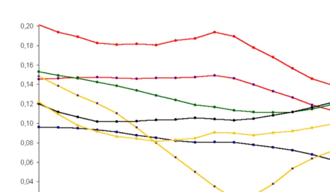
Figure 4 depicts the trends in distances from the age structure of the US white non-Hispanic female population to the age structures of other race-origin groups [source of data: U.S. Bureau of the Census 2000a, 2000b]. The following abbreviations for the race-origin groups are used in the figures and the text:

Abbreviation used Description

WhNonHis White, non-Hispanic female population BlNonHis Black, non-Hispanic female population

AmNonHis American Indian, Eskimo, and Aleut, non-Hispanic female population AsNonHis Asian and Pacific Islander, non-Hispanic female population

Wh Hisp White, Hispanic female population Bl Hisp Black, Hispanic female population

Am Hisp American Indian, Eskimo, and Aleut, Hispanic female population As Hisp Asian and Pacific Islander, Hispanic female population

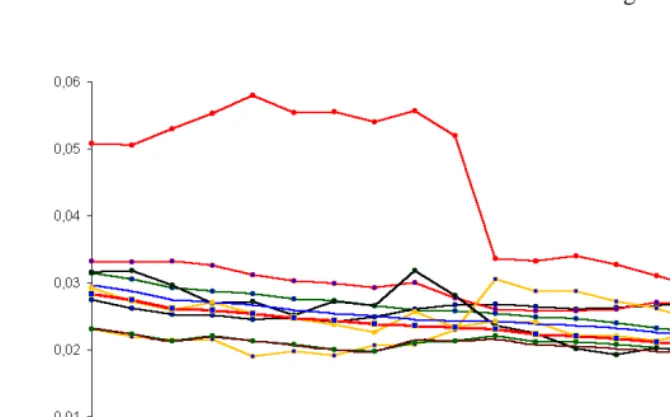
Figure 4: Distances between age structures of the US race-origin groups and the structure of the US White non-Hispanic female population, 1980-2000

Notable racial differentials can be observed on figure 4. Although 90s became a decade of convergence in structures of different races, sufficient nonzero distances still persist. While the Hispanic origin plays an important role for Whites, Blacks, and Asian and Pacific Islanders, American Indian, Eskimo, and Aleuts seem to be more homogeneous. Another conclusion, which can be made, is that the US whites and blacks seem to be close to each other given the same origin status. These race groups were converging to each other during 80s and especially during 90s. At the same time both blacks and whites with Hispanic origin were diverging from the appropriate race group with non-Hispanic origin, i.e. their demographic behavior was persistently and sufficiently dependent on original status. It worth to compare these distances to the dynamics of the race-origin groups’ age structures, which can be reflected by the distance from the population’s structure to its own structure one year later:

( )

( )

( )

( )

∑

=

+

+

−

⋅

X

x

x x x

t

V

t

n

t

V

t

n

v

0

1

1

{32}

may be caused by the discontinuity of demographic statistics before and after the 1990 census. Yet, the American Indian, Eskimo, and Aleut, Hispanic female population deserves further research on causes of the unusual trend during 80s.

Figure 5: Dynamics of age structures of the US race-origin groups, 1980-2000

Table 8.3: Distances between the US race-origin groups as of year 2000

WhNonHis BlNonHis AmNonHis Am Hisp Wh Hisp Bl Hisp As Hisp AsNonHis

WhNonHis 0.04 0.09 0.10 0.13 0.12 0.10 0.09

BlNonHis 0.04 0.06 0.08 0.12 0.11 0.08 0.11

AmNonHis 0.09 0.06 0.05 0.14 0.14 0.11 0.15

Am Hisp 0.10 0.08 0.05 0.12 0.12 0.10 0.14

Wh Hisp 0.13 0.12 0.14 0.12 0.03 0.06 0.12

Bl Hisp 0.12 0.11 0.14 0.12 0.03 0.04 0.11

As Hisp 0.10 0.08 0.11 0.10 0.06 0.04 0.10

AsNonHis 0.09 0.11 0.15 0.14 0.12 0.11 0.10

In addition to the trends presented, it is useful to look to the pattern of interracial distances as of 2000 (table 8.3.) The authors’ experience in working with the monotonic measures suggests that the distances of 0.05 or less can be attributed to the natural random variations in birth numbers, which are observed in any real population. Observing the distances between the racial groups can help in aggregating them into a few relatively uniform subgroups of the US population. According to these distances the US races can be arranged into the following groups with presumably close demographic characteristics (these groups are highlighted in table 8.3):

- Non-Hispanic Whites and Blacks and all American Indian, Eskimo, and Aleuts. - All Hispanic groups except for American Indian, Eskimo, and Aleuts with Hispanic origin.

- Asian and Pacific Islander, non-Hispanic female population.

One could also use the more detailed classification of the race groups:

- Non-Hispanic Whites and Blacks. - All American Indian, Eskimo, and Aleuts.

- All Hispanic groups except for American Indian, Eskimo, and Aleuts with Hispanic origin.

- Asian and Pacific Islander, non-Hispanic female population.

Either one of the classifications presented can be used to build reproduction models for the US population, which reflect the heterogeneity of the population on the one hand, and the similarity of demographic characteristics on the other hand.

9. Acknowledgements

References

Arthur, W. B. (1981). “Why a Population Converges to Stability.” American Mathematical Monthly, 88, 8: 557-563.

Arthur, W. B. (1982). “The Ergodic Theorems of Demography: a Simple Proof.” Demography, 19: 439-445.

Ediev, D. M. (1999). Demographic and economic-demographic potentials. Ph. D. thesis. Moscow: Moscow Institute of Physics and Technology.

Ediev, D. M. (2000). “Principles of aggregate economic-demographic modeling based on demographic potentials’ technique.” In: Demographic-macroeconomic modeling (workshop). Rostock: Max-Planck Institute for Demographic Research, 2000. 17 pp. www.demogr.mpg.de/Papers/workshops/ws001011.htm

Ediev, D. M. (2001a). “Application of the Demographic Potential Concept to Understanding the Russian Population History and Prospects: 1897-2100.” Demographic Research, Vol. 4, Article 9: 289-336. http://www.demographic-research.org/volumes/vol4/9/4-9.pdf

Ediev, D. M. (2001b). “Aggregate Population Forecasting With the Use of Demographic Potentials Technique.” Investigated In Russia (Demographic section), 38e: 408-431. http://zhurnal.ape.relarn.ru/articles/2001/038e.pdf

Ediev, D. M. (2001c). “Reconstruction of the US immigration history: demographic potential approach.” Investigated In Russia 'HPRJUDSKLFVHFWLRQ 1635.

http://zhurnal.ape.relarn.ru/articles/2001/140e.pdf

Ediev, D. M. (2002a). “On conditions of monotonic convergence of population structure to the structure of stable equivalent population in Kullback distance within the model of reproduction of demographic potential.” Investigated in Russia (Demographic section), 17: 182-190. http://zhurnal.ape.relarn.ru/articles/2002/017.pdf

Ediev, D. M. (2002b). “Interrelations between the spectrum of Leslie matrix and the age pattern of demographic potentials.” Investigated In Russia (Demographic VHFWLRQ KWWS]KXUQDODSHUHODUQUXDUWLFOHV SGI Ediev, D. M. (2002c). “On conditions of monotonic convergence of population

Fisher, R. A. (1930). The genetical theory of natural selection. N. -Y. : Dover Publications.

Golubitsky, M. , Keeler, E. B. , and Rothschild, M. (1975). “Convergence of the Age Structure: Applications of the Projective Metric.” Theoretical Population Biology, 7: 84-93.

Hardy, G. H. , Littlewood, J. E. , Polya, G. (1934). Inequalities. Cambridge.

Keyfitz, N. (1969). “Age Distribution and Stable Equivalent”. Demography, 6: 261-269.

Keyfitz, N. , Flieger, W. (1990). World Population Growth and Aging: Demographic Trends in the Late Twentieth Century. Chicago and London: The University of Chicago Press.

Kullback, S. , Leibler, R. (1951). “On information and Sufficiency.” Ann. of Math. Stat., 22: 79-86.

Kullback, S. (1959). Information theory and statistics. New York: John Wiley. (Reprinted by Dover, New York, 1968).

Leslie, P. H. (1945). “On the use of matrices in certain population mathematics.” Biometrika, XXXV: 183-212.

Leslie, P. H. (1948). “Some Further Notes on the Use of Matrices in Population Mathematics”. Biometrika, XXXV: 213-245.

Polyak, B. T. (1983). Introduction to the optimization. Moscow: Nauka.

Rubinov, A. M., Chistyakova, N. E. (1986). “Age structure and the potential of population growth”. In: Volkov, A. G. (Editor). Demographic processes and their regularities. Moscow: Mysl, 1986. Pp. 38-52.

Pirozhkov, S. I. (1976). Demographic processes and the age structure of the population. Moscow: Statistika.

Schoen R. , Kim, Y. J. (1991). “Movement toward stability as a fundamental principle of population dynamics.” Demography, 28: 455-466.

Tuljapurkar, S. D. (1982). “Why use population entropy? It determines the rate of convergence.” Journal of Mathematical Biology, 13: 325-337.

http://www.census.gov/population/www/projections/popproj.html Internet Release Date: January 13, 2000. Last Revised Date: January 19, 2001.

U. S. Bureau of the Census. (2000b). U. S. Population Estimates by Age, Sex, Race, and Hispanic Origin: 1980 to 1999 (With short-term projections to dates in 2000). http://eire.census.gov/popest/estimates.php Internet Release Date: April 11, 2000.

United Nations. (1983). Manual X. Indirect techniques for demographic estimation. N. Y. : UN.

Appendix: Numerical results for illustrative examples presented in

the text

Table A1: Dynamics of different distances to the stable equivalent for the female population of Austria, 1985-2100. Projection is made using 1985 vital rates and under zero migration. [Keyfitz and Flieger 1990: 404-405].

Kullback Abs Abs^2 Abs^4 Kullback Abs Abs^2 Abs^4

1985 0,005595 0,456838 0,060023 0,001572 100,00 100,00 100,00 100,00

1990 0,003687 0,348863 0,039929 0,000748 65,89 76,36 66,52 47,57

1995 0,002640 0,293884 0,028475 0,000408 47,19 64,33 47,44 25,92

2000 0,001718 0,218466 0,018363 0,000230 30,71 47,82 30,59 14,64

2005 0,001043 0,172529 0,011121 0,000114 18,65 37,77 18,53 7,23

2010 0,000640 0,149686 0,006869 0,000047 11,44 32,77 11,44 2,96

2015 0,000393 0,116929 0,004249 0,000016 7,02 25,60 7,08 1,05

2020 0,000271 0,103718 0,002944 0,000005 4,84 22,70 4,90 0,35

2025 0,000193 0,089900 0,002092 0,000002 3,45 19,68 3,49 0,13

2030 0,000127 0,068506 0,001373 0,000001 2,27 15,00 2,29 0,06

2035 0,000089 0,059242 0,000963 0,000000 1,59 12,97 1,60 0,03

2040 0,000061 0,049981 0,000660 0,000000 1,09 10,94 1,10 0,01

2045 0,000040 0,040493 0,000438 0,000000 0,72 8,86 0,73 0,01

2050 0,000029 0,035871 0,000315 0,000000 0,52 7,85 0,52 0,00

2055 0,000020 0,029216 0,000213 0,000000 0,35 6,40 0,35 0,00

2060 0,000013 0,024268 0,000144 0,000000 0,24 5,31 0,24 0,00

2065 0,000009 0,021228 0,000103 0,000000 0,17 4,65 0,17 0,00

2070 0,000006 0,016397 0,000068 0,000000 0,11 3,59 0,11 0,00

2075 0,000004 0,013794 0,000047 0,000000 0,08 3,02 0,08 0,00

2080 0,000003 0,011845 0,000033 0,000000 0,06 2,59 0,06 0,00

2085 0,000002 0,008856 0,000022 0,000000 0,04 1,94 0,04 0,00

2090 0,000001 0,007578 0,000016 0,000000 0,03 1,66 0,03 0,00

2095 0,000001 0,006411 0,000011 0,000000 0,02 1,40 0,02 0,00

2100 0,000001 0,005012 0,000007 0,000000 0,01 1,10 0,01 0,00

Table A2: Dynamics of different measures for convergence between the female population of Austria and the population initially consisting of persons at ages 10-20; 1985-2100. Projection is made using 1985 Austrian vital rates and under zero migration [Keyfitz and Flieger 1990: 404-405].

Kullback Abs Abs^2 Abs^4 Kullback Abs Abs^2 Abs^4

1985 -0,365534 6,745271 9,176343 21,414729 -100,00 100,00 100,00 100,00

1990 -0,231117 6,011895 7,970232 19,041740 -63,23 89,13 86,86 88,92

1995 -0,194056 5,019124 6,123267 14,176936 -53,09 74,41 66,73 66,20

2000 -0,172929 4,212380 4,319862 8,320280 -47,31 62,45 47,08 38,85

2005 -0,126961 3,108090 2,585005 3,820660 -34,73 46,08 28,17 17,84

2010 -0,039200 2,456206 1,545148 1,446963 -10,72 36,41 16,84 6,76

2015 0,025564 2,079714 1,018522 0,509810 6,99 30,83 11,10 2,38

2020 0,042106 1,556879 0,664658 0,208963 11,52 23,08 7,24 0,98

2025 0,040943 1,329521 0,470510 0,100029 11,20 19,71 5,13 0,47

2030 0,032600 1,132445 0,332995 0,048576 8,92 16,79 3,63 0,23

2035 0,022238 0,864793 0,219266 0,022838 6,08 12,82 2,39 0,11

2040 0,015400 0,752694 0,155634 0,010617 4,21 11,16 1,70 0,05

2045 0,010074 0,636143 0,107137 0,005021 2,76 9,43 1,17 0,02

2050 0,006512 0,517248 0,071226 0,002364 1,78 7,67 0,78 0,01

2055 0,004701 0,458359 0,051147 0,001117 1,29 6,80 0,56 0,01

2060 0,003233 0,372372 0,034482 0,000534 0,88 5,52 0,38 0,00

2065 0,002195 0,309649 0,023307 0,000251 0,60 4,59 0,25 0,00

2070 0,001556 0,270597 0,016716 0,000118 0,43 4,01 0,18 0,00

2075 0,001018 0,208310 0,011092 0,000056 0,28 3,09 0,12 0,00

2080 0,000702 0,175352 0,007663 0,000027 0,19 2,60 0,08 0,00

2085 0,000501 0,150400 0,005435 0,000013 0,14 2,23 0,06 0,00

2090 0,000332 0,112682 0,003579 0,000006 0,09 1,67 0,04 0,00

2095 0,000234 0,096585 0,002524 0,000003 0,06 1,43 0,03 0,00

2100 0,000162 0,081700 0,001757 0,000001 0,04 1,21 0,02 0,00

‘Kullback’ stands for the Kullback information distance; ‘Abs’ stands for the weighted sum of age-specific absolute deviations from stable equivalent; ‘Abs^2’ stands for the weighted sum of age-specific quadratic deviations; and ‘Abs^4’ stands for the weighted sum of age-specific deviations in the 4th

Table A3: Dynamics of different distances to the stable equivalent for the female population of Austria, 1985-2100. Projection is made using 1985 vital rates and under zero migration. [Keyfitz and Flieger 1990: 404-405]. Standard reproductive values are used (Table 8.2), which doesn’t relate to the actual vital rates used in projections.

Kullback Abs Abs^2 Abs^4 Kullback Abs Abs^2 Abs^4

1985 -0,006188 0,551197 0,082583 0,003122 -100,00 100,00 100,00 100,00

1990 0,000595 0,416336 0,052646 0,001380 9,62 75,53 63,75 44,20

1995 0,006414 0,349754 0,036431 0,000636 103,65 63,45 44,11 20,38

2000 0,006244 0,266471 0,024171 0,000334 100,90 48,34 29,27 10,71

2005 0,001428 0,213661 0,015726 0,000184 23,08 38,76 19,04 5,89

2010 -0,001827 0,180508 0,010116 0,000092 -29,53 32,75 12,25 2,95

2015 -0,001311 0,137323 0,006172 0,000042 -21,19 24,91 7,47 1,34

2020 0,000892 0,118772 0,003925 0,000015 14,41 21,55 4,75 0,48

2025 0,001819 0,103462 0,002649 0,000004 29,40 18,77 3,21 0,13

2030 0,000909 0,081315 0,001808 0,000002 14,69 14,75 2,19 0,06

2035 -0,000431 0,070475 0,001278 0,000001 -6,96 12,79 1,55 0,03

2040 -0,000848 0,058775 0,000869 0,000000 -13,71 10,66 1,05 0,01

2045 -0,000226 0,047299 0,000579 0,000000 -3,66 8,58 0,70 0,01

2050 0,000475 0,041644 0,000410 0,000000 7,67 7,56 0,50 0,00

2055 0,000523 0,034152 0,000279 0,000000 8,44 6,20 0,34 0,00

2060 0,000067 0,028414 0,000189 0,000000 1,08 5,16 0,23 0,00

2065 -0,000296 0,024733 0,000134 0,000000 -4,79 4,49 0,16 0,00

2070 -0,000245 0,019354 0,000090 0,000000 -3,96 3,51 0,11 0,00

2075 0,000038 0,016296 0,000062 0,000000 0,62 2,96 0,08 0,00

2080 0,000201 0,013913 0,000044 0,000000 3,24 2,52 0,05 0,00

2085 0,000119 0,010552 0,000029 0,000000 1,92 1,91 0,04 0,00

2090 -0,000051 0,009003 0,000020 0,000000 -0,83 1,63 0,02 0,00

2095 -0,000117 0,007559 0,000014 0,000000 -1,88 1,37 0,02 0,00

2100 -0,000046 0,005927 0,000009 0,000000 -0,74 1,08 0,01 0,00

‘Kullback’ stands for the Kullback information distance; ‘Abs’ stands for the weighted sum of age-specific absolute deviations from stable equivalent; ‘Abs^2’ stands for the weighted sum of age-specific quadratic deviations; and ‘Abs^4’ stands for the weighted sum of age-specific deviations in the 4th