Coarse Graining Method Based on Hierarchical Clustering on Complex Networks

(1)

ISSN Online: 1947-3826 ISSN Print: 1949-2421

DOI: 10.4236/cn.2019.111003 Feb. 22, 2019 21 Communications and Network

Coarse-Graining Method Based on Hierarchical

Clustering on Complex Networks

Lin Liao, Zhen Jia

*

, Yang Deng

College of Science, Guilin University of Technology, Guilin, China

Abstract

With the rapid development of big data, the scale of realistic networks is in-creasing continually. In order to reduce the network scale, some coarse-graining methods are proposed to transform large-scale networks into mesoscale net-works. In this paper, a new coarse-graining method based on hierarchical clustering (HCCG) on complex networks is proposed. The network nodes are grouped by using the hierarchical clustering method, then updating the weights of edges between clusters extract the coarse-grained networks. A large number of simulation experiments on several typical complex networks show that the HCCG method can effectively reduce the network scale, mean-while maintaining the synchronizability of the original network well. Fur-thermore, this method is more suitable for these networks with obvious clus-tering structure, and we can choose freely the size of the coarse-grained net-works in the proposed method.

Keywords

Complex Network, Synchronizability, Coarse-Graining Method, Hierarchical Clustering

1. Introduction

Our life is full of all kinds of networks. For example, metabolic networks, large- scale power networks, paper citation networks, global transportation networks, scientific research cooperation networks and so on. These networks have same analogous and obvious characteristics—massive nodes and complex interac-tions. Networks with complex topological properties are called complex net-works [1]. A complex network is formed by abstracting the basic units of a com-plex system into nodes and the interactions between the units into edges. Com-plex networks are important tools for studying the relationship between the

How to cite this paper: Liao, L., Jia, Z. and Deng, Y. (2019) Coarse-Graining Method Based on Hierarchical Clustering on Com-plex Networks. Communications and Net-work, 11, 21-34.

https://doi.org/10.4236/cn.2019.111003

Received: January 18, 2019 Accepted: February 19, 2019 Published: February 22, 2019

http://creativecommons.org/licenses/by/4.0/

(2)

DOI: 10.4236/cn.2019.111003 22 Communications and Network

structure and function of complex systems.

The existed research methods of complex networks are mainly designed for mesoscale networks. Coarse-graining technology is an effective way to study the large-size networks, which can reduce the complexity of networks by merging similar nodes. However, coarse-graining techniques go far beyond the require-ment of clustering techniques, because coarse-graining techniques requires the coarse-grained networks to keep the initial network’s topological properties or dynamic characteristics, such as the degree distribution, clustering coefficient, correlation properties [2], random walk properties [3], synchronizability [4]. In 2007, Gfeller et al., proposed a spectral coarse-graining (SCG) algorithm, which is based on the eigenvalue spectrum of random walk probability matrix, the al-gorithm can maintain the random walk characteristics of original networks [5]. In 2008, Gfeller et al. further used SCG technology on the Laplace matrix of networks to extract coarse-grained networks, while maintaining the synchroniza-bility of original networks [6]. In 2013, J Chen et al. [7] studied the coarse-graining method on the networks with obvious clustering structure in literature [5] [6]: through a large number of simulation experiments on WS small world networks, ER random networks, and BA scale-free networks, we can draw the conclusion that the clustering structure of networks can enhance the coarse-graining effect. In 2016, Shuang Xu et al. proposed a coarse-graining method based on K-means clustering which by redistributing the central cluster nodes of the network and clustering to reduce the network scale, the method can keep some statistical characteristics of initial networks in some extent, such as degree distribution, assortativity and so on [9]. In 2017, the ISCG [8] algorithm proposed by our re-search group Zhou et al., the algorithm adopt split clustering method determin-ing which nodes should be are grouped together, the algorithm can effectively keep the synchronizability of original networks, and the effect is better than SCG method in directed networks. Recently, our research team proposed a spectral coarse-graining method based on K-means clustering, by numerical simulations, they find that this method has better effect in preserving the synchronizability of original networks than SCG algorithm. Xingbo Liu proposed a cohesive hierar-chical clustering algorithm based on variable merging threshold, and gave a ref-erence formula for the distance threshold [10].

(3)

More-DOI: 10.4236/cn.2019.111003 23 Communications and Network

over, this method does not need to define the objective function and does not cause the problem of selecting the initial point. The new coarse-graining method can make up for some shortcomings of the above-mentioned methods. In the HCCG method, we use the hierarchical clustering method to cluster the network nodes, and update the weights of edges between clusters to extract the coarse- grained network. Furthermore, we apply the HCCG method to WS small world networks, ER random networks and BA scale-free networks. Simulation experi-ments show that the HCCG method can keep the synchronizability of the initial network well, and the method is more suitable for the networks with more ob-vious clustering structure.

The rest of the paper is organised as follows. In Section 2, the mathematical basis of the HCCG method is introduced. The steps of the HCCG method are presented in Section 3. In Section 4, a large number of numerical simulations on several typical networks verify the feasibility and effectiveness of the proposed method. Finally, conclusions and discussion are drawn in Section 5.

2. Mathematical Basis

2.1. Hierarchical Clustering Algorithm

Clustering is an unsupervised learning process. By clustering, the similarity is as large as possible in the same cluster and as small as possible in different clusters. The fundamental difference between sorting technique and clustering technique is that sorting technique must know the data characteristic on which it is based in advance, and the clustering technique is to find the data characteristics. Therefore, clustering analysis is usually used as a data preprocessing process in many fields, which is the basis for further data analysis and processing [11]. There are usually four clustering methods: partitioning methods, hierarchical methods, density-based methods, and grid-based methods [12]. In this paper, we use the hierarchical methods to cluster networks nodes.

Hierarchical clustering methods merge or separate data objects recursively until some termination condition met. According to the order of hierarchical decomposition, the method can be divided into bottom-up algorithm and top- down algorithm. This paper adopts the bottom-up method, which is a cohesive hierarchical clustering algorithm. The algorithm starts with every individual as a cluster, then searching for the nearest cluster to group into one cluster. After merging once, the total number of clusters is reduced by one, until the required number of clusters or the nearest threshold is reached. In this paper, Jaccard distance is used to calculate the distance between two different nodes. The me-thods of calculating the distance between two different clusters include Single Linkage, Complete Linkage, Average Linkage and so on. In this paper, we use the Average Linkage in the HCCG method.

(

)

{

}

, 1 ,

i j

avg i j

p C p C i j

dist C C p p

n n ∈ ′∈

′

=

∑

− ₍₁₎

(4)

nodes of the initial network, the coarse-grained network has N _clusters,

la-beled with C=1,2, , N , Ci is the label of the cluster of node i, Ci is the

cardinality of the set Ci, ni = Ci (ni is the number of nodes in the cluster i

C ).

2.2. Index of Network Synchronizability

Consider an unweighted and undirected network with N nodes, A

( )

aij N N

×

= _is

the adjacency matrix of the network,

( )

aii =0 and

( ) ( )

aij = aji =1 if node i

connects to j

(

i j≠

)

_{, otherwise}

( ) ( )

aij = aji =0. D diag k k=

(

1, , ,2 kN

)

is a

diagonal matrix, ki is the degree of i’th node. L D A= − , L=

( )

L_{ij N N}_× ∈RN N×

is the Laplacian matrix of the network. L satisfies the dissipative coupling condi-tion:

∑

iN=₁Lij =0. Since the network is connected, L is a symmetric matrix with

nonnegative eigenvalues: 0=λ1 <λ2 ≤≤λN.

Generally, according to the difference of synchronization regions, network systems can be divided into four types, each type corresponds to a kind of syn-chronization region: 1) Type-I networks correspond to bounded regions

(

α α1, 2

)

;

2) Type-II networks correspond to unbounded regions

(

α1,∞

)

; 3) Type-III

networks correspond to union of several bounded regions ∪

(

α α1i, 2i

)

; 4) Type-

IV networks correspond to empty sets. Generally, the networks of the case (3) and (4) are difficult or impossible to achieve synchronization. Fortunately, most networks are in the case of (1) and (2). In Type-I networks, The synchronizabil-ity of networks can be characterized by the minimum non-zero eigenvalue λ2.

The larger the value of λ2, the smaller the coupling strength is needed to

achieve synchronization, the synchronizability of Type-I networks are stronger. In Type-II networks, the synchronizability of networks can be characterized by the ratio of λ λ2 N . Only when the eigenvalues ratio λ λ2 N >α α1 2 are

satis-fied can the network achieve synchronization. So, the larger the value of

2 N

R=λ λ , the stronger the synchronizability of Type-II networks. Therefore, if

2

λ _or λ λ₂ _N is unchanged in the process of coarse-graining, we can deem the synchronizability of the network is maintained [13].

3. Hierarchical Clustering Coarse-Graining Scheme

There are three main steps in the HCCG method: the first step is calculating the distance between two nodes for obtaining the distance matrix of the initial net-work by using Jaccard distance, and constructing n single-member clusters; the second is calculating the distance between two different clusters, using the hie-rarchical clustering method to cluster the network nodes; the last step is updat-ing the weight of the links between different clusters to extract the coarse-grained network. In this section, the HCCG scheme is introduced revolving around the above content.

3.1. Jaccard Distance Calculation

(5)

the cardinality of the set ϑ

( )

i . ϑ

( )

i =ki, ki are the degrees of nodes i. The

Jaccard coefficient is defined as follows:

( )

ij

i j i j

J

i j i j i j

ϑ ϑ ϑ ϑ

ϑ ϑ ϑ ϑ ϑ ϑ

= =

+ −

∩ ∩

∪ ∩ (2)

here, i j, are two different nodes. ϑ

( )

i ∩ϑ

( )

j is the common neighbor nodes set of node i and j, ϑ

( )

i ∪ϑ

( )

j is the union of the neighbor nodes of node i

and j. When ϑ

( )

i =0_and ϑ

( )

j =0_, Jij =1. Jaccard distance is an index

related to Jaccard coefficient. The lower the nodes similarity, the larger the Jac-card distance. The JacJac-card distance is defined as follows:

( )

1

ij ij

i j i j

d J

i j

ϑ ϑ ϑ ϑ

ϑ ϑ

− = − = ∪ ∩

∪ (3)

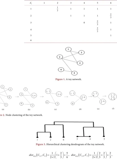
A toy network is used to illustrate how to calculate the distance between two different nodes, using Jaccard distance method obtain the Table 1.

In Figure 1, ϑ

( ) { }

1 = 3,4 , ϑ

( ) {

2 = 3,4,5

}

, ϑ

( ) { }

3 = 1,2 , ϑ

( ) { }

4 = 1,2 ,

( ) { }

5 2,6

ϑ = _,ϑ

( ) { }

6 = 5 _._{Table 1}_{can be obtained based on Equation (3).}

3.2. Node Clustering of Networks

The basic idea of hierarchical clustering method is to calculate the similarity between nodes by some similarity index, and to rank the nodes according to the similarity from high to low, then to merge the nodes step by step. The main steps are as follows:

1) Obtain the adjacency matrix A of the network;

2) Use Jaccard distance method calculating the distance between two different nodes to obtain the distance matrix of the network, construct n single-member clusters, the height of each cluster is 0;

3) Use Average Linkage method calculating the distance between two different clusters to search for the nearest clusters C Ci, j, merging C Ci, j, reducing the

number of all clusters by 1, take the distance between the two clusters merged as the height of the upper layer;

4) Calculate the distance between the newly generated cluster and other clus-ters in this layer. If the termination condition is satisfied, the algorithm will end, otherwise it will turn to (3).

To better explain the steps of clustering, we use the example in Figure 2, a 6-node toy network is clustered into one cluster. The obtained hierarchical clus-tering dendrogram is shown in Figure 3.

In Table 1, the closest distance is d3,4=0 on the Figure 2(a), so node 3

and node 4 are grouped together; based on Equation (3), we know d1,2 =1₃ is

the minimum distance on the Figure 2(b), so node 1 and node 2 are grouped together; according to Equation (1),

(

1,2, 3,4

)

_{2 2}1

(

1 1 1 1 1

)

avg

dist C C = + + + =

(6)

Table 1. Distance matrix of the toy network.

ij

d 1 2 3 4 5 6

1 1₃ 1 1 1 1

2 1 1 1 2

3

3 0 2₃ 1

4 2

3 1

5 1

6

Figure 1. A toy network.

[image:6.595.124.537.88.647.2]

Figure 2. Node clustering of the toy network.

Figure 3. Hierarchical clustering dendrogram of the toy network.

(

1,2, 6

)

_{2 1}1 1 2₃ 5₆

avg

dist C C = _ + _=

×   ,

(

3,4 5

)

1 2 2 2

,

2 1 3 3 3

avg

dist C C = _ + _= ×   ,

(

3,4, 6

)

_{2 1}1

(

1 1 1

)

avg

dist C C = + =

× , distavg

(

C C5, 6

)

=_{1 1}1_×

(

1 1 1+ =

)

,

the nearest distance is distavg

(

C C3,4, 5

)

=2₃ on the Figure 2(c), the cluster of

3,4

(7)

(

1,2, 3,4,5

)

_{2 3}1

(

1 1 1 1 1 1 1

)

avg

dist C C = + + + + + =

× ,

(

1,2, 6

)

_{2 1}1 1 2₃ 5₆

avg

dist C C = _ + _=

×   ,

(

3,4,5 6

)

(

)

1

, 1 1 1 1

3 1 avg

dist C C = + + =

× ,

the nearest distance is distavg

(

C C1,2, 6

)

=5₆ on the Figure 2(d), so the cluster of

1,2

C and node 6 are grouped together; according to Equation (1), the nearest distance is

(

1,2,6, 3,4,5

)

_{3 3}1

(

1 1 1 1 1 1 1 1 1 1

)

avg

dist C C = + + + + + + + + =

×

on the Figure 2(e), all nodes are grouped together into one cluster.

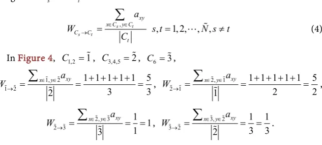
3.3. Updating Edges of the Coarse-Grained Network

Clusters are obtained according to the clustering steps which in Section 3.2, then based on the Equation (4) update the edge weight between different clusters to extract the coarse-grained network. C Cs, t are two different clusters, and the

weight of Cs to Ct are defined as:

, _, _{1,2, , ,}

s t s t

xy x C y C

C C

t

a

W s t N s t

C ∈ ∈ → = = ≠

∑

(4)

In Figure 4, C1,2 =1, C3,4,5=2, C6 =3,

1, 2 1 2

1 1 1 1 1 5

3 3

2 xy

x y a

W ∈ ∈

→ + + + + =

∑

= = , 2, 1 2 1

1 1 1 1 1 5

2 2

1 xy

x y a

W ∈ ∈

→

+ + + +

=

∑

= =

,

2, 3

2 3 ₃ 1 1₁

xy

x y a

W ∈ ∈

→ = = =

∑

, 3 2 3, 2

1 1 3 3 2

xy

x y a

W ∈ ∈

→ = = =

∑

.

4. Application and Simulation

In this section, we apply the HCCG method to several typical complex networks. The several types of networks including: WS small world networks, ER random networks and BA scale-free networks. N is the size of initial networks; N _{is the}

size of coarse-grained networks, λ2 is the minimum non-zero eigenvalue of the

[image:7.595.210.538.334.482.2]

coarse-grained network, R=λ λ2 N is the eigenvalue ratio of the coarse-grained

(8)

network. The closer the values of λ2 and λ2 (or R and R), the better the

ef-fect of the HCCG method on keeping the synchronizability of original networks.

4.1. WS Small World Network

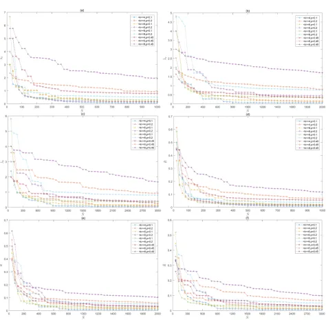
In 1998, Watts and Strogatz [14] [15] proposed the algorithm for the formation of small world networks and established WS model, found that most real net-works have short average path lengths and high clustering coefficients. The WS network is based on the random edge rewiring of regular networks, which stipu-lated that there mustn’t be self-ring and multiple edges. Random reconnection probability p=0 corresponds to complete regular networks and p=1 cor-responds to complete random networks. By adjusting the value of p, the transi-tion from regular networks to random networks can be realized. Figures 5(a)-(c)

shows the evolution curves of λ2 by using the HCCG method in WS small

world networks with initial sizes N=1000,2000,3000 respectively, and Fig-ures 5(d)-(f) shows the evolution curves of R by using the HCCG method in WS small world networks with initial sizes N=1000,2000,3000 respectively. For each cases, networks with average degrees k =4,6,8_{and rewiring}

proba-bilities p=0.1,0.2,0.45 are considered. Each simulation result was obtained by 5 independent repeated experiments.

As shown in Figures 5(a)-(c), in Type-I networks, when p=0.1,0.2_, 4,6,8

k = _{the synchronizability of original networks can be maintained well}

in the coarse-graining process. However, with the increasing of p, the effect has not been so good. When the p value is fixed, the smaller the k , the better the effect of the HCCG method. In the literature [16]: The clustering structure of networks contribute to improve the synchronicity of coarse-graining methods. The construction algorithm of WS small world model starts with the regular graph, at this time, on each nodes left and right sides is connected with k 2

adjacent nodes respectively, the clustering structure of the network is clear rela-tively, it is effective to keep the synchronizability of the original network by us-ing the HCCG method; then the network is reconnected randomly with proba-bility p. With the increasing of p and p, the clustering structure becomes weaker. The reason is that: k ×p is the number of the nodes randomly reconnected, when the network scale is fixed, the larger p and p are, the more random recon-nected nodes, the weaker the clustering structure. Therefore, the smaller the

k and p, the better the efect of the HCCG method.

As shown in Figures 5(d)-(f), in Type-II networks, the evolution curves of

R_{are consistent with that of} _λ₂_{. The reason is also consistent with in the case}

of Type-I networks. The difference is: when k and p are quite large, the effect of the HCCG method in Type-II networks is better than that in Type-I networks.

When p increases gradually, The minimum non-zero eigenvalue λ2 and the

maximum eigenvalue λN increase simultaneously, λ2 increases much faster

than λN which lead to the rise in R=λ λ2 N [17], so with p increases the

(9)

[image:9.595.64.539.58.525.2]

Figure 5. (a)-(c) Evolution of λ2 by using the HCCG method in WS small world network; (d)-(f) Evolution of R by using the HCCG method in WS small world network.

k and p, the clustering structure of the network becomes weaker, the effect of maintaining original network’s synchronizability becomes not so good. So the HCCG method is more suitable for the networks with obvious clustering struc-ture.

4.2. ER Random Network

In 1959, Erdos and Renyi, two Hungarian mathematicians, proposed algorithm for the formation of random graphs [18]. The ER random graph G N p

(

,

)

giv-en N nodes firstly, the connecting probability between any two different points is

(10)

[image:10.595.64.540.56.519.2]

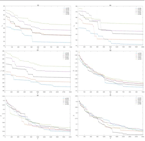
Figure 6. (a)-(c) Evolution of λ2 by using the HCCG method in ER random network; (d)-(f) Evolution of R by using the HCCG method in ER random network.

HCCG method in ER random networks with initial sizes N=1000,2000,3000

respectively, and Figures 6(d)-(f) shows the evolution curves of R_{by using}

the HCCG method in ER random networks with initial size N=1000,2000,3000

respectively. For each case, the connecting probability is

0.26,0.35,0.47,0.67,0.88

p= _{. Each simulation result was obtained by 5}

inde-pendent repeated experiments.

The eigenvalue spectral distribution of ER random networks is symmetrical, and as the connection probability p increases, the range of eigenvalue distribu-tion shrinks rapidly, at the same time, λ2 and λN increase. The main reason

(11)

faster than that of λN, which leads to the increase of R=λ λ2 N . Therefore,

from a view of statistical perspective, the synchronizability is gradually increased as the connection probability p increases [19]. Figures 6(a)-(c), in Type-I net-works, when the size of the coarse-grained network is larger than or equal to that of original network’s 60 percent, although the difference of the value λ2 is

quite big in the case of different p, the method can maintain the synchronizabil-ity of the original network well. We can see that the larger p, the larger the value of λ2. So the larger p, the stronger the synchronizability of the network. The

minimum size (that can maintain the synchronizability of original network) in the case of p=0.88_{is significantly smaller than that in the case of} p=0.26_.

Therefore, the larger p, the better the effect of the HCCG method, which is con-sistent with the reference [19]. As shown in Figures 6(d)-(f), in Type-II net-works, the HCCG method also can maintain the synchronizability of the original network well. So, the HCCG method is suitable for ER networks.

4.3. BA Scale-Free Network

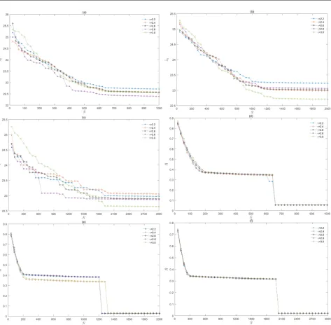
In 1999, Baralsi and Albert established BA model to explain the scale-free prop-erty of complex networks [19] [20]. They believed that most complex systems in the real world evolve dynamically, and these complex systems are open and self-organizing. Scale-free phenomena in real networks comes from two tant factors: Growth pattern and Priority connection mode. Another an impor-tant discovery in network science research is that the degree distribution of net-works can be described by appropriate power-law form. The degrees of nodes in these networks have no obvious characteristic length, so these networks are called scale-free networks. Figures 7(a)-(c) shows the evolution curves of λ2

by using the HCCG method in BA scale-free networks with initial sizes

1000,2000,3000

N= respectively, and Figures 7(d)-(f) shows the evolution curves of R_{by using the HCCG method in BA scale-free networks with initial}

sizes N =1000,2000,3000 respectively. The larger the power-law exponents γ

of the network, the weaker the heterogeneity. In the real complex networks, γ

mostly range among 2 and 3. So we main consider the networks with power-law exponents γ =2.2,2.4,2.6,2.8,3.0_{, Each simulation result was obtained by 5}

independent repeated experiments.

(12)

[image:12.595.64.538.57.521.2]

Figure 7. (a)-(c) Evolution of λ2 by using the HCCG method in BA scale-free network; (d)-(f) Evolution of R by using the HCCG method in BA scale-free network.

networks, with the increasing of average degree, the synchronizability of the network basically unchanged. ER random networks have some emergence prop-erties: for any given connecting probability p, either almost every graph G N p

(

,

)

has a certain nature Q, or almost every graph G N p

(

,

)

does not have this property Q. The suddenly increasing of R _{whether mean that arising certain}

emergence properties in BA scale-free networks, the problem has yet to be stu-died.

5. Conclusion and Discussion

(13)

complex networks. In the HCCG method, the distance and similarity are defined simply. Jaccard distance is used to obtain the distance matrix of the network. Average Linkage method is used to find the nearest clusters. We use the hierar-chical clustering method to cluster the network nodes, and update the weights of edges between clusters to extract the coarse-grained network. Massive simula-tion experiments show the HCCG method can keep the synchronizability of the original network well, and the method more suitable for the network with ob-vious clustering structure. Furthermore, the size of coarse-grained networks can be chosen freely in the HCCG method. However, the suddenly increasing of R

on BA scale-free network whether mean that certain emergence properties aris-ing, the problem has yet to be studied. In addition, greedy algorithm is used in hierarchical clustering, thence the clustering result is local optimum, may not be global optimum, the problem can be solved by adding random effects, which is also the direction of our future researches.

Acknowledgements

This project was supported by National Natural Science Foundation of China (Nos. 61563013, 61663006) and the Natural Science Foundation of Guangxi (No. 2018GXNSFAA138095).

Conflicts of Interest

The authors declare no conflicts of interest regarding the publication of this pa-per.

References

[1] Jin, Y.P. (2016) Coarsening and Anomaly Detection of Complex Networks. (In Chinese)

[2] Kim, B.J. (2004) Geographical Coarse Graining of Complex Networks. Physical Re-view Letters, 93, 168701. https://doi.org/10.1103/PhysRevLett.93.168701

[3] Weiss, G.H. and Havlin, S. (1986) Some Properties of a Random Walk on a Comb Structure. Physica A Statistical Mechanics and Its Applications, 134, 474-482.

https://doi.org/10.1016/0378-4371(86)90060-9

[4] Duan, Z., Chen, G. and Huang, L. (2007) Complex Network Synchronizability: Analysis and Control. Physical Review E Statistical Nonlinear and Soft Matter Physics, 76, 056103. https://doi.org/10.1103/PhysRevE.76.056103

[5] Gfeller, D. and Rios, P.D.L. (2007) Spectral Coarse Graining of Complex Networks. Physical Review Letters, 99, 038701. https://doi.org/10.1103/PhysRevLett.99.038701

[6] Gfeller, D. and Rios, P.D.L. (2008) Spectral Coarse Graining and Synchronization in Oscillator Networks. Physical Review Letters, 100, 174104.

https://doi.org/10.1103/PhysRevLett.100.174104

[7] Zhou, J., Jia, Z. and Li, K.Z. (2017) Improved Algorithm of Spectral Coarse Grain-ing Method of Complex Network. Acta Physica Sinica.

(14)

[9] Shuang, X. and Pei, W. (2016) Coarse Graining of Complex Networks: A k-Means Clustering Approach. Control and Decision Conference.

[10] Liu, X.B. (2008) Research on the Clustering Algorithm of Cohesive Hierarchy. Scientific and Technological Information: Scientific Teaching and Research, 11, 202. (In Chinese)

[11] Duan, M.X. (2009) Research and Application of Hierarchical Clustering Algo-rithms. Central South University. (In Chinese)

[12] Zhang, J.H. (2007) K-Means Clustering Algorithms Research and Application. Wuhan University of Technology, Wuhan. (In Chinese)

[13] Anonymous (2012) Introduction to Network Science. (In Chinese)

[14] Watts, D.J. (1999) Networks, Dynamics, and the Small-World Phenomenon. Amer-ican Journal of Sociology, 105, 1-10. https://doi.org/10.1086/210318

[15] Watts, D.J. (1999) Small Worlds: The Dynamics of Networks between Order and Randomness. Princeton University Press, Princeton.

[16] Chen, J., Lu, J.A., Lu, X.F., Wu, X.Q. and Chen, G.R. (2013) Spectral Coarse Grain-ing of Complex Clustered Networks. Communications in Nonlinear Science and Numerical Simulation, 18, 3036-3045. https://doi.org/10.1016/j.cnsns.2013.03.020

[17] Chen, J. and Lu, J. (2012) Medium-Scale Study of Complex Networks Uncovers the Process of Network Synchronization. Journal of University of Electronic Science and Technology, 41. (In Chinese)

[18] Erdos, P. and Rnyi, A. (1960) On the Evolution of Random Graphs. Publication of the Mathematical Institute of the Hungarian Academy Offences, 38, 17-61. [19] Barabasi, A.L. and Albert, R. (1999) Emergence of Scaling in Random Networks.

Science, 286, 509-512.

[20] Barabasi, A.L., Albert, R. and Jeong, H. (1999) Mean-Field Theory for Scale-Free Random Networks. Physica A, 272, 173-187.

https://doi.org/10.1016/S0378-4371(99)00291-5