Mapping spatial variability of soil properties and yield by using geostatic method

One of the key elements of the precision agricul-ture is mapping the crop yields. Variability in crop yield is the basic source variable for the majority of other inputs. In addition to this, the yield data pro-vide initial information on the respective land.

At the present time, the issue of technical facilities needed to secure a variable application has already been solved relatively well. One of the factors limiting the commercial spread of the precision agriculture is still the price of sampling that needs to be performed to such an extent allowing to compile maps. Soil be-longs to the most variable matrices that are sampled in the environment (Sáňka 1998). If we intend to use the measuring data to describe the spatial rela-tions, we have to perform sampling with a sufficient resolution. The grab sampling is applied frequently, however, it cannot be used for describing the spatial distribution of values in many cases (Basso et al. 2003). Precision sensoric methods will have to be developed to replace labor- and time-consuming sampling methods (Hanquet et al. 2004). Therefore, the sensing equipment is being developed intensively at the present time with the aim to provide a high resolution measuring at minimum costs.

MATERIALS AND METHODS

Two sites were selected for performing experi-ments, first one with an area of 21 ha (Kuchař) and

second one with an area of 26 ha (Bora-left), in Nové Strašecí locality. The sites are managed by the Lány-based CUA Farm established by the Czech Univer-sity of Agriculture in Prague. The spatial properties of yield data, electric conductivity of soil, and pulling forces necessary to apply the soil tillage equipment were examined through geostatistical methods.

The yield was monitored during the perennial wheat harvest campaign. Commercially available yield meters were used for measuring the yield, the principle of which is based on detecting the dura-tion of light beam interrupdura-tion. The yield meter was installed on the Claas reaper-thresher.

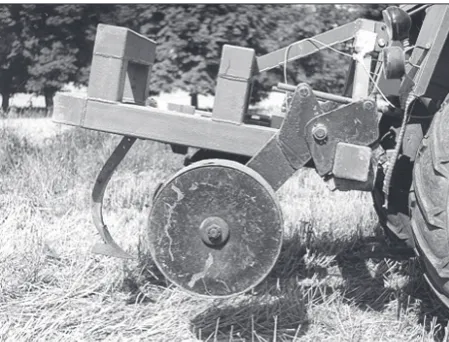
Dynamometric measuring method was applied to determine the tensile (horizontal) element of the tillage equipment force. The force requirements for towing a single share (Figure 1) were observed. Pull-ing force data were recorded each 5 seconds in the data logging center including the machine position. Position data were obtained using GPS unit. The contact measuring method was applied for detect-ing the soil conductivity. Measurdetect-ing instrument was developed by the Department of Machinery Appli-cation, Technical Faculty of the Czech University of Agriculture in Prague (Figure 2). Voltage and current data together with the position data were recorded each 5 seconds by the data logging center.

Geostatistical calculations and interpolations were carried out using the following software: GS+

Supported by the Ministry of Education, Youth and Sports of the Czech Republic, Project No. MSM 604 6070905.

Mapping spatial variability of soil properties

and yield by using geostatic method

M. Kroulík

_{, M. Mimra}

_{, F. Kumhála}

_{, V. Prošek}

1

_{Department of Agricultural Machines, Technical Faculty, Czech University}  

of Agriculture in Prague, Prague, Czech Republic

2

_{Department of Machinery Utilisation, Technical Faculty, Czech University}  

of Agriculture in Prague, Prague, Czech Republic

Abstract: The Czech University of Agriculture in Prague (CUA) Farm at Lány started with precision farming technol-ogy several years ago. In the first step the yield and nutrients content were monitored. For precision application devel-opment, detailed description of soil conditions and interrelationship will be necessary. Pulling force and soil electric conductivity measurement as indirect measuring methods were used for mapping spatial soil variability. These methods demonstrate other ways for description of complex soil media.

ver. 5.1.1, ArcGIS 9 with Geostatistical Analyst add-on.

RESULTS AND DISCUSSION

Three data sets were obtained from each site, which included the yield, conductivity and tensile force data. Several modifications were performed on the initial data set prior to statistical processing and evaluation. As stated by Thylén et al. (1997), the majority of errors occur when the machine starts a new line. Thus, values that did not describe precisely the factor measured were removed from the initial data set, e.g. errors possibly occurring when recess-ing the tillage equipment. These values were elimi-nated by trimming the marginal points recorded. Values larger then double of the average were also excluded from the initial data set.

The time series was smoothened during subse-quent modification. According to Hayhoe et  al. (2002), the values show oscillations from the curve. A simple running average method was applied to smoothen the time series of all measurements. The following formula was used:

1

Y_t = – (Y_t–1 + Y_t + Y_{t + 1) (1)}

3

where: Y – original values at time t.

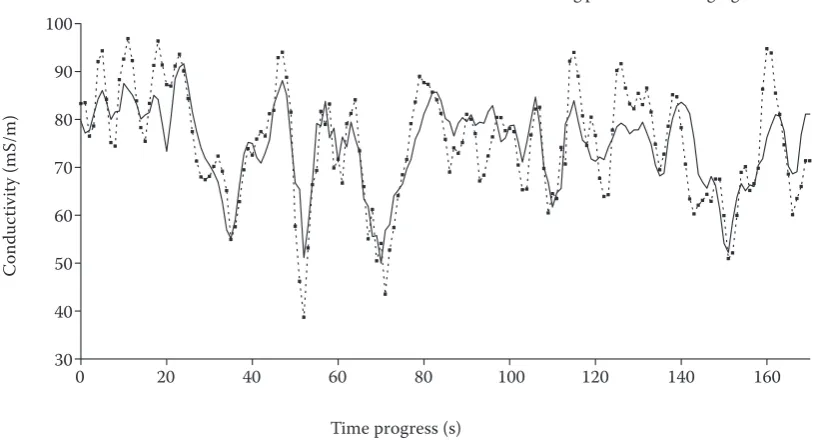
Average for value in the following instant of time is calculated after obtaining the average in given time point. Figure 3 illustrates an extract from the time se-ries of conductivity values for Bora-left site. Original and transformed values were included in the graph. Figure suggests that distribution of values is not of a random nature, but rather follows a continuous curve. Statistical properties of transformed values for both sites are provided in Tables 1 and 2.

The range of values expressed by the maximum and minimum values as well as variation coefficient values illustrate variability of the individual data sets. Asymmetry from the normal distribution is ex-pressed by the coefficient of asymmetry. According to Granados et al. (2002), the normality condition is met, if the interval of inclination lays between –2 and 1. Low inclination values prove that data show a normal distribution. The inclination value of 1 was only exceeded by yield values obtained for Figure 1. Pulling force measuring frame instruments Figure 2. Soil conductivity measuring

0 50 100 150

0 20 40 60 80 100 120 140 160

Time progress (s)

C

on

du

ct

iv

ity

(m

S/

m

)

original values smoothened data

+ original values smoothened data

Time progress (s)

0 20 40 60 80 100 120 140 160

C

on

du

ct

iv

ity

(m

S/

m

)

150

100

50

0

Kuchař site. Owing to a negligible exceeding and fact that distribution normality is not a pre-requisite of geostatistical processing, the original data set was processed without any transformation.

Modified data were processed using geostatisti-cal methods. Variogram parameters were used for describing the spatial relationships. Experimental variograms were calculated for all values. Obtained variograms were then interleaved with model vari-ograms. Interleaving was carried out based on the R2

determination parameters and sum of squares of RSS residues, which express the tightness and reliability of interleaving. Parameters of variograms for both sites are illustrated on Figures 4 and 5. The basic vari-ogram parameters are listed in Tables 3 and 4.

Spherical and exponential models with a residual variance (nugget) were used for interleaving the experimental variograms. The nugget effect was not detected only for conductivity values. Appro-priateness of selected models is proved by the low Table 1. Statistical properties of transformed data for Bora-left site

Variable/Property _(t/ha)Yield Conductivity _(mS/m) Pulling force _(kN)

Mean value 8.02 68.88 3.40

Median 8.06 68.61 3.37

Standard deviation 0.99 12.09 0.37

Variance of selection 0.98 146.29 0.14

Variation coefficient (%) 12.32 17.56 10.84

Acuteness 1.97 0.09 0.65

Inclination 0.29 0.08 0.54

Minimum 4.59 32.49 2.28

Maximum 14.41 110.54 4.81

Quantity 7453.00 789.00 1706.00

Table 2. Statistical properties of transformed data for Kuchař site

Variable/Property _(t/ha)Yield Conductivity _(mS/m) Pulling force _(kN)

Mean value 7.61 57.23 3.78

Median 7.47 57.71 3.77

Standard deviation 1.24 7.91 0.43

Variance of selection 1.54 62.63 0.19

Variation coefficient (%) 20.23 109.44 4.98

Acuteness 2.51 1.37 1.00

Inclination 1.06 –0.66 0.17

Minimum 4.02 20.67 2.28

Maximum 13.49 78.69 5.34

Quantity 5469.00 383.00 998.00

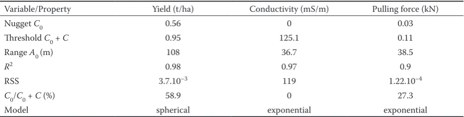
Table 3. Parameters of model variograms, Bora-left site

Variable/Property Yield (t/ha) Conductivity (mS/m) Pulling force (kN)

Nugget C₀ 0.56 0 0.03

Threshold C₀ + C 0.95 125.1 0.11

Range A₀ (m) 108 36.7 38.5

R2 _{0.98 0.97 0.9}

RSS 3.7.10–3 _{119 1.22.10}–4

C₀/C₀ + C (%) 58.9 0 27.3

values of parameters, which express the tightness of interleaving. Growth of semi-variance was observed after reaching the threshold values for conductivity values. This phenomenon mostly indicates spatial relation of the value monitored for larger distances. These relationships, however, were not observed.

Value A₀ represents the variogram range. Value of spatial relation is reflected at this point. Similar values of range were observed for pulling force. Differences for other values were caused especially by using various variogram models. Threshold value for exponential models has been determined

mathematically. Values of range, thus, vary con-siderably.

The spatial relation itself is expressed as a share of the residual variance (C₀) in the total threshold value (C₀ + C). Distribution of spatial relations into classes can be found e.g. in Granados et al. (2002), and Cambardella and Karlen (1999). Magnitude of the spatial relation is expressed as a ratio of the nug-get value to the total sill of the variogram. If this ratio is ≤ 25%, we are talking about strong spatial relation. Values between 25% and 75% express medium spa-tial relation. Values exceeding 75% express spaspa-tially 0.95 0.72 0.48 0.24 0 γ (h ) Y ie ld (t /h a) 2

0 50 100 150

0.11 0.09 0.06 0.03 0 γ (h ) P ul lin g fo rc e (k N 2)

0 50 100 150

125 94 63 31 0 γ (h ) C on du ct iv ity (m S/ m ) 2

0 50 100 150

1.49 1.12 0.75 0.37 0 γ (h ) Y ie ld (t /h a) 2

0 50 100 150

0.17 0.13 0.08 0.04 0 γ (h ) P ul lin g fo rc e (k N 2)

0 50 100 150

56 42 28 14 0 γ (h ) C on du ct iv ity (m S/ m ) 2

0 50 100 150

Figure 4. Variograms of data sets for Bora-left site Figure 5. Variograms of data sets for Kuchař site

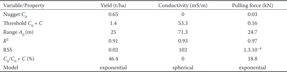
Table 4. Parameters of model variograms, Kuchař site

Variable/Property Yield (t/ha) Conductivity (mS/m) Pulling force (kN)

Nugget C₀ 0.65 0 0.03

Threshold C₀ + C 1.4 53.3 0.16

Range A₀ (m) 25 71.3 24.7

R2 _{0.91 0.93 0.97}

RSS 0.02 102 1.3.10–4

C₀/C₀ + C (%) 46.4 0 18.8

independent data. If the ratio equals to 100%, we are talking about pure nugget, as mentioned above. High values of spatial relation were observed for con-ductivity and pulling force values. The pulling force value for Bora-left site is on the limit between high and medium values. Medium spatial relation was ob-served for yield values. This result results especially

3.9–5.9 5.9–7.0 7.0–7.5 7.5–7.8 7.8–8.0 8.0–8.2 8.2–8.8 8.8–9.8 9.8–11.9 11.9–15.8

15–51 51–57 57–61 61–64 64–68 68–72 72–75 75–80 80–87 87–129

1.2–2.8 2.8–3.0 3.0–3.1 3.1–3.2 3.2–3.3 3.3–3.4 3.4–3.5 3.5–3.7 3.7–3.9 3.9–5.3 Yield (t/ha)

Conductivity (mS/m)

Pulling force (kN) N

N N

0 65 130 260 390

0 65 130 260 390

0 65 130 260 390

m m m

3.5–5.2 5.2–6.2 6.2–6.8 6.8–7.1 7.1–7.3 7.3–7.7 7.7–8.3 8.3–9.3 9.3–11.0 11.0–13.9 Yield (t/ha)

N

0 50 100 200 300

m

13–32 32–44 44–51 51–55 55–58 58–60 61–62 62–66 66–74 74–85 Conductivity (mS/m)

N

0 50 100 200 300

m

from a higher value of the residual variance. Residual variance represents a value of semi-variance with the distance of points close to 0. It is attributed to measuring errors or variability on the lower level than is the smallest distance between two points measured. For yield values this was probably con-nected especially with the inaccuracy of measuring

1.0–3.2 3.2–3.4 3.4–3.5 3.5–3.6 3.6–3.7 3.7–3.8 3.8–4.0 4.0–4.2 4.2–4.5 4.5–6.3 Pulling force (kN)

N

0 50 100 200 300

m

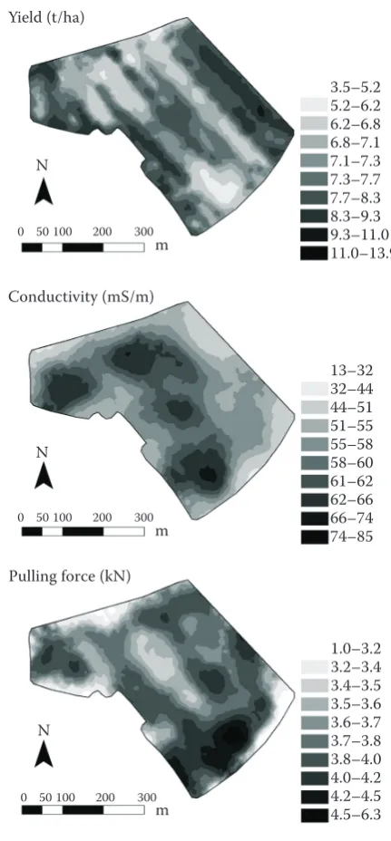
Figure 6. Maps of values obtained for Bora-left site Figure 7. Maps of values obtained for Kuchař site

Table 5. Statistical characterisation of residues based on estimates obtained from Kriging method, Bora-left site

Variable/Property _(t/ha)Yield Conductivity _(mS/m) Pulling force _(kN)

Mean value 0.015 0.066 0.001

Median 0.039 0.159 0.006

Standard deviation 0.746 6.396 0.252

using optical sensor. The pulling force values, where residual variance was also observed, were probably influenced by the variability of the soil environment. Tensile force may be affected by micro-variability of the soil environment, which occurs at a distance of even few centimeters. This force cannot be covered due to the measurement intervals.

The actual output of the geostatistical processing are maps illustrating spatial distribution of values measured. Maps presented were created using Krig-ing interpolation method. This is a weighted average

method, where weights of individual values deter-mine variogram parameters.

Individual maps are presented on Figures 6 and 7. Darker colors always represent higher values of given parameter.

There are smaller delimited surfaces of different colors in the maps. This indicates high resolution of maps given by the high measuring density.

Validation of model values, or interpolation of data obtained respectively, is performed using the Cross-validation method. This method eliminates

30 40 50 60 70 80 90 100

0 20 40 60 80 100 120 140 160

Time progress (s)

Conductivity

(mS/m)

Measuring points Kriging

Time progress (s)

0 20 40 60 80 100 120 140 160

Kriging Measuring points

C

on

du

ct

iv

ity

(m

S/

m

)

100

90

80

70

60

50

40

30

5 6 7 8 9 10 11

0 20 40 60 80 100 120 140 160

Time progress (s)

Yi

el

d

(t/

ha

)

Measuring points Kriging

Time progress (s)

0 20 40 60 80 100 120 140 160

Kriging Measuring points

Yi

el

d

(t/

ha

)

11

10

9

8

7

6

5

Figure 8. Map section for yield – Kriging method, Bora-left site

the original value and calculates a new value using the Kriging method for a particular point. Differ-ences between measured and estimated values are expressed by average error (MEE), variance (MSE), and standard deviation (SMSE) (Granados et al. 2002; Miao et al. 2003). Statistical characteristics of errors of interpolation method estimates were ob-tained. As stated by Brodský (2003), it is paramount that the distribution of residues, or their mean value respectively, approaches to zero and that variance and standard deviation are low.

Tables 6 and 7 indicate that the condition of a low mean value was complied with. Also standard devia-tion and variadevia-tion values are low and there are small

differences between individual pairs of values, with the exception of conductivity. Differences in variance and standard deviation values were caused by the selected type of variogram.

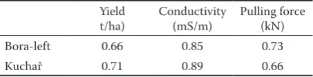
Relevance of an estimate can also be identified through correlation analysis between measured and estimated values. Coefficient of correlation R should equal to 1 in an ideal case.

Table showing coefficients of correlation also documents the accuracy of estimate obtained through interpolation method. Influence of vari-ogram parameters is also profound, especially influence of the residual variance to the estimate quality. Highest values of correlation coefficient were achieved for conductivity, where zero residual variance was observed. Correlation coefficient de-creased gradually with growing residual variance value. Map section may also be used for better visual representation. As already stated earlier, the course is influenced by variogram parameters for Kriging method. This can be seen on sections shown on Figures 8–10.

Table 6. Statistical characterization of residues based on estimates obtained from Kriging method, Kuchař site

Variable/Property _(t/ha)Yield Conductivity _(mS/m) Pulling force _(kN)

Mean value –0.004 0.075 0.002

Median –0.024 –0.002 0.011

Standard deviation 0.869 3.722 0.325

Variance of selection 0.756 13.856 0.106

2.0 2.5 3.0 3.5 4.0 4.5 5.0

0 20 40 60 80 100 120 140 160 180

Time progess (s)

Pulling

force

(k

N)

Measuring points Kriging

Time progress (s)

0 20 40 60 80 100 120 140 160 180

Kriging Measuring points

Pu

lli

ng

fo

rc

e

(k

N

)

5.0

4.5

4.0

3.5

3.0

2.5

2.0

Figure 10. Map section for pulling force – Kriging method, Bora-left site Table 7. Summary of results from correlation analysis between

measured and estimated values

Yield

t/ha) Conductivity (mS/m) Pulling force (kN)

Bora-left 0.66 0.85 0.73

CONCLUSION

Geostatistical methods were applied gradually to six data sets obtained from two sites managed by the Lány-based CUA Farm. Indirect measuring methods were used for measuring and the following values were determined: yield, soil conductivity, and pulling force. Statistical analysis showed variability of values within individual sites.

Geostatistical methods were used for monitoring the spatial relations. Spatial relations were identified for all data sets based on a result of spatial relation-ship analysis utilising the C₀/(C₀ + C) ratio. Strong spatial relation was identified for conductivity val-ues. Pulling force and yield values showed medium spatial relation.

Spatial distribution of values was illustrated by maps. Relevance of the Kriging spatial interpolation estimate was validated through the Cross-validation method. Significance of variogram modeling for the subsequent interpolation was proven.

Indirect methods represent an important ele-ment of the precision agriculture and will play an important role in the continued development of this technology. Appropriate attention shall be paid to research in this field.

References

Basso B., Sartori L., Bertocco M., Oliviero G. (2003): Evaluation of variable depth tillage: economic aspects and simulation of long term effects on soil organic matter and soil physical properties. In: Proc. 4th _{European Conference}

on Precision Agriculture, Wageningen Academic Publish-ers, Wageningen, 61–67.

Brodský L. (2003): Využití geostatistických metod pro ma-pování prostorové variability agrochemických vlastností půd. ČZU Praha, Praha, 120.

Cambardella C.A., Karlen D.L. (1999): Spatial analysis of soil fertility parameters. Precision Agriculture, 1: 5–14. Granados F.L., Expósito J.M., Atenciano S., Ferrer A.G.,

Sánchez De La Orden M., Torres L.G. (2002): Spatial variability of agricultural soil parameters in southern Spain. Plant and Soil, 246: 97–105.

Hanquet B., Sirjacobs D., Destain M.F., Frankinet M., Verbrugge J.C. (2004): Analysis of soil variability mea-sured with a soil strength sensor. Precision Agriculture, 5: 227–246.

Hayhoe H.N., Lapen D.R., McLaughlin N.B. (2002): Mea-surements of mouldboard plow draft: I. Spectrum analysis and filtering. Precision Agriculture, 3: 225–236.

Miao Y., Robert P.C., Mulla D.J. (2003): Geostatistical analyst of soil properties and corn quality. In: Proc. 4th Eu-ropean Conference on Precision Agriculture, Wageningen Academic Publishers, Wageningen, 417–423.

Sáňka M. (1998): Vzorkování půd pro jednorázová šetření a dlouhodobá pozorování. Sborník Odběr, skladování a zpracování půdních vzorků, ÚPB AV ČR, České Budě-jovice, 7–9.

Thylén L., Jürschnik P., Murphy D. (1997): Improving the quality of yield data. Precision Agriculture, BIOS Scientific Publishers Ltd., Oxford, UK, 743–750.

Received for publication November 9, 2005 Accepted after corrections January 10, 2006

Abstrakt

Kroulík M., Mimra M., Kumhála F., Prošek V. (2006): Mapování prostorových vlastností půdy a výnosu s využitím geostatistických metod. Res. Agr. Eng., 52: 17–24.

Školní zemědělský podnik ČZU v Lánech začal využívat technologii precizního zemědělství již před několika lety. Nejdříve byly sledovány výnosy a obsah živin. Pro použití variabilních aplikací je však nezbytné znát detailně půdní podmínky a jejich vzájemné vztahy. Měření tahového odporu a elektrické vodivosti se využilo jako nepřímé metody pro mapování prostorové variability půdy. Tyto metody představují další způsob pro popis prostorové variability.

Klíčová slova: precizní zemědělství; geostatistika; mapy; prostorová variabilita

Corresponding author:

Ing. Milan Kroulík, Ph.D., Česká zemědělská univerzita v Praze, Technická fakulta, katedra zemědělských strojů, Kamýcká 129, 165 21 Praha 6-Suchdol, Česká republika