ABSTRACT
BANG, JISU. Characterization of Soil Spatial Variability for Site-Specific Management Using Soil Electrical Conductivity and Other Remotely Sensed Data (Under the direction of Jeffrey G. White and Randy Weisz).
Field-scale characterization of soil spatial variability using remote sensing technology has potential for achieving the successful implementation of site-specific management (SSM). The objectives of this study were to: (i) examine the spatial relationships between apparent soil electrical conductivity (ECa) and soil chemical and physical properties to determine if ECa could be useful to characterize soil properties related to crop productivity in the Coastal Plain and Piedmont of North Carolina; (ii) evaluate the effects of in-situ soil moisture variation on ECa mapping as a basis for characterization of soil spatial variability and as a data layer in cluster analysis as a means of delineating sampling zones; (iii) evaluate clustering approaches using different variable sets for management zone delineation to characterize spatial variability in soil nutrient levels and crop yields. Studies were conducted in two fields in the Piedmont and three fields in the Coastal Plain of North Carolina. Spatial measurements of ECa via electromagnetic induction (EMI) were compared with soil chemical parameters
increments to 0.75 m using profiling time-domain reflectometry probes to evaluate the temporal variability of ECa associated with changes in in situ soil moisture content. Nonhierarchical k-means cluster analysis using sensor-based field attributes including vertical ECa, near-infrared (NIR) radiance of bare-soil from an aerial color infrared (CIR) image, elevation, slope, and their combinations was performed to delineate management zones.
The strengths and signs of the correlations between ECa and measured soil properties varied among fields. Few strong direct correlations were found between ECa and the soil chemical and physical properties studied (r2 < 0.50), but correlations improved considerably when zone mean ECa and zone means of selected soil properties among ECa zones were compared. The results suggested that field-scale ECa survey is not able to directly predict soil nutrient levels at any specific location, but coulddelimit distinct zones of soil condition among which soil nutrient levels differ, providing an effectivebasis for soil sampling on a zone basis.
The strengths of the correlations of ECa with measured soil properties varied depending on soil moisture conditions. In general, the strongest correlations were observed when ECa was measured under relatively dry conditions. The results suggest that the spatial and temporal ECa variability measured under different soil moisture conditions could be a critical factor when evaluating the ability of ECa to predict soil chemical and physical characteristics important to soil and crop productivity and management.
CHARACTERIZATION OF SOIL SPATIAL VARIABILITY FOR SITE-SPECIFIC MANAGEMENT USING SOIL ELECTRICAL CONDUCTIVITY
AND OTHER REMOTELY SENSED DATA
by
JISU BANG
A dissertation submitted to the Graduate Faculty of North Carolina State University
in partial fulfillment of the requirements for the Degree of
Doctor of Philosophy
SOIL SCIENCE
Raleigh, NC 2005
Approved by:
Dr. Marcia L. Gumpertz Dr. Deana Osmond
(Advisory Committee Member) (Advisory Committee Member)
BIOGRAPHY
ACKNOWLEDGMENTS
I would like to express my deep gratitude to my major advisor, Dr. Jeffrey G. White, who entrusted this project to me over the past three years. His professional and personal relationship during the course of this project have been a great asset in my pursuit of this research. I would like to thank Dr. Randall Weisz for his support and guidance provided throughout this study. I would like to acknowledge my committee members, Dr. Deana Osmond and Dr. Marcia L. Gumpertz, for their dedication to this study. Their comments and ideas have helped make this a great project.
I would like to acknowledge Dr. D. Keith Cassel, Dr. Crowell Bowers, and Mindy Lohman for supplying data. Dr. Jim Thompson was very helpful with the creation of the digital elevation models. Lastly, I would like to thank Dr. David Hardy for helping with the soil test analyses at the North Carolina Department of Agriculture and Consumer Services Soil Testing Laboratory.
Thanks to the NCSU Department of Soil Science for providing me the
opportunity to pursue my Ph.D. degree in a warm and friendly atmosphere of academic excellence and for providing a place to call home. Thank you to Brian Roberts, Wesley Childres, and Chris Niewoehner for aiding me in my field efforts and setting things in the right perspective. I am grateful to Laura Overstreet and Jared Williams who shared office space with me. Your friendship has been a valuable part of my experience at NC State.
TABLE OF CONTENTS
LIST OF TABLES ... vii
LIST OF FIGURES ... xii
CHAPTER ONE: INTRODUCTION AND LITERATURE REVIEW ... 1
INTRODUCTION ... 2
Apparent Soil Electrical Conductivity (ECa) ... 4
Management Zones ... 8
Landscape Attributes Related to Yields and Soil Properties ... 11
Aerial Soil Imagery in SSM... 12
Cluster Analysis ... 15
SUMMARY... 19
REFERENCES ... 21
CHAPTER TWO: SPATIAL RELATIONSHIPS BETWEEN APPARENT SOIL ELECTRICAL CONDUCTIVITY AND SOIL PROPERTIES: IMPLICATIONS FOR MANAGEMENT ZONE DELINEATION ... 33
ABSTRACT... 34
INTRODUCTION ... 36
MATERIALS AND METHODS... 39
Field Description ... 39
Data Collection... 40
Statistical Analysis ... 44
RESULTS AND DISCUSSION ... 46
Spatial Variability of ECa and Soil Chemical and Physical Properties... 46
Direct Relationships between ECa and Soil Chemical Properties... 48
Direct Relationships between ECa and Soil Physical Properties ... 53
CONCLUSIONS... 57
REFERENCES ... 59
CHAPTER THREE: CHARACTERIZING FIELD-SCALE SOIL ELECTRICAL CONDUCTIVITY-SOIL MOISTURE RELATIONS FOR SITE-SPECIFIC MANAGEMENT... 111
ABSTRACT... 113
INTRODUCTION ... 115
MATERIALS AND METHODS... 118
Field Description... 118
Apparent Soil Electrical Conductivity and Water Content Measurements ... 119
Spatial and Temporal Variability of Soil Moisture Content ... 126
Effects of Soil Moisture on Spatial and Temporal Variability of Apparent Soil Electrical Conductivity ... 128
Effects of Spatiotemporal Variation of Soil Moisture Content on Characterizing Soil Properties using Apparent Soil Electrical Conductivity... 131
Effects of Spatiotemporal Variation of Soil Moisture Content on Management Zone Approaches Incorporating Apparent Soil Electrical Conductivity... 135
CONCLUSIONS... 140
REFERENCES ... 142
CHAPTER FOUR: EFFECTS OF VARIABLE SELECTION ON SOIL-BASED MANAGEMENT ZONE STRATEGIES: CLUSTER ANALYSIS APPROACH... 179
ABSTRACT... 181
INTRODUCTION ... 183
MATERIALS AND METHOD... 188
Field Description... 188
Acquisition of Spatial Data Layers ... 189
RESULTS AND DISCUSSION ... 195
Spatial Variability of Selected Soil Properties and Sensor-Based Field Attributes... 195
Relationships among Soil Fertility Parameters, Sensor-based Field Attributes, and Crop Yields... 198
Management Zone Delineation via Cluster Analysis: ... 202
Effects of Variable Selection on the Capture of Spatial Variability of Soil Properties... 202
Effects of Variable Selection on the Capture of Spatial Variability of Crop Yield... 207
CONCLUSIONS... 209
LIST OF TABLES
CHAPTER TWO: SPATIAL RELATIONSHIPS BETWEEN APPARENT SOIL ELECTRICAL CONDUCTIVITY AND SOIL PROPERTIES:
IMPLICATIONS FOR MANAGEMENT ZONE DELINEATION
Table 2. 1. Field descriptions for the five study fields...64 Table 2. 2. Descriptive statistics of horizontal and vertical apparent soil electrical
conductivity (ECa) measurements in three coastal plain and two piedmont
fields...67 Table 2. 3. Descriptive statistics of selected soil chemical properties in three
coastal plain and two piedmont fields...68 Table 2. 4. Significant (p ≤ 0.05) correlation coefficients (r) between horizontal
and vertical apparent soil electrical conductivity (ECa) and selected soil
chemical parameters in three coastal plain and two piedmont fields...70 Table 2. 5. Field-scale apparent soil electrical conductivity (ECa) zone means and
significance for soil test P, K, pH, cation exchange capacity (CEC), and humic matter (HM) or soil organic matter (SOM) measured in the five study fields. Zones were generated from k-means cluster analysis of vertical ECa surveys. Differences among means were tested using PROC MIXED with a
best-fit spatial covariance model. ...71 Table 2. 6. Significant (p ≤ 0.05) correlation coefficients (r) between horizontal
and vertical apparent soil electrical conductivity (ECa) and percentage sand,
silt, and clay in three coastal plain fields and two piedmont fields. ...73 Table 2. 7. Significant (p ≤ 0.05) correlation coefficients (r) between apparent
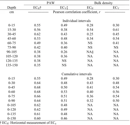
soil electrical conductivity (ECa) and soil physical parameters of plant available water (PAW) and bulk density measured at individual and
cumulative depth intervals in the Schoolteacher field (n = 80). ...75 APPENDIX TABLE A
Table A. 1. Significant (p ≤ 0.05) correlation coefficients (r) between horizontal and vertical measurement of apparent soil electrical conductivity (ECa); green, red, and NIR bands; elevation; slope; and selected measured soil
chemical properties (n = 467) in the Kinston field...97 Table A. 2. Significant (p ≤ 0.05) correlation coefficients (r) between horizontal
and vertical measurement of apparent soil electrical conductivity (ECa); green, red, and NIR bands; elevation; slope; and selected measured soil
chemical properties (n = 342) in the Overman field...98 Table A. 3. Significant (p ≤ 0.05) correlation coefficients (r) between horizontal
and vertical measurement of apparent soil electrical conductivity (ECa); green, red, and NIR bands; elevation; slope; and selected measured soil
chemical properties (n = 100) in the Schoolteacher field. ...99 Table A. 4. Significant (p ≤ 0.05) correlation coefficients (r) between horizontal
Table A. 5. Significant (p ≤ 0.05) correlation coefficients (r) between horizontal and vertical measurement of apparent soil electrical conductivity (ECa); green, red, and NIR bands; elevation; slope; and selected measured soil
chemical properties (n = 361) in the Graham field. ...101 Table A. 6. Descriptive statistics of percentage sand, silt, and clay (n = 60) for
individual and cumulative depth intervals in the Kinston field. ...102 Table A. 7. Descriptive statistics of percentage sand, silt, and clay (n = 50) for
individual and cumulative depth intervals in the Overman field...103 Table A. 8. Descriptive statistics of percentage sand, silt, and clay (n = 50) for
individual and cumulative depth intervals in the Schoolteacher field. ...104 Table A. 9. Descriptive statistics of percentage sand, silt, and clay (n = 50) for
individual and cumulative depth intervals in the Baker field. ...105 Table A. 10. Descriptive statistics of percentage sand, silt, and clay (n = 50) for
individual and cumulative depth intervals in the Graham field...106 Table A. 11. Field-scale apparent soil electrical conductivity (ECa) zone means
and significance for soil test P, K, pH, CEC, and HM measured in the five study fields. Zones were generated from k-means cluster analysis of vertical
ECa surveys. Differences among zone means were tested using PROC GLM...107 Table A. 12. Significant (p ≤ 0.05) correlation coefficients (r) between apparent
soil electrical conductivity (ECa) and percentage sand, silt, and clay measured at individual depth intervals in three coastal plain fields and two
piedmont fields...109
CHAPTER THREE: CHARACTERIZING FIELD-SCALE SOIL ELECTRICAL CONUCTIVITY-SOIL MOISTURE RELATIONS FOR SITE-SPECIFIC
MANAGEMENT
Table 3. 1. Descriptive statistics of coastal plain field apparent soil electrical conductivity (ECa) measured via electromagnetic induction under four
different naturally occurring soil moisture conditions...148 Table 3. 2. Correlation matrix of field apparent soil electrical conductivity (ECa)
measured via electromagnetic induction in the vertical mode under four different naturally occurring soil moisture conditions. Correlation
coefficients (r) listed in this table are significant at the 0.05 probability level. ...149 Table 3. 3. Semivariogram model parameters (nugget, sill, range) of vertical ECa
Table 3. 5. Significant (p ≤ 0.05) correlation coefficients (r) between soil
physical parameters and apparent soil electrical conductivity (ECa) measured
under four different naturally occurring soil moisture conditions (n = 60). ...152 Table 3. 6. Significant (p ≤ 0.05) correlation coefficients (r) between selected
surficial soil chemical parameters and apparent soil electrical conductivity (ECa) measured under four different naturally occurring soil moisture
conditions (n = 564)...154 Table 3. 7. Means and significance of field-scale apparent soil electrical
conductivity (ECa) zones and control zones for soil test P, K, pH, CEC, and SOM. Zones were generated from k-means cluster analysis of four
individual ECa surveys under different naturally occurring soil moisture conditions. Control zones were generated from cluster analysis of X, Y coordinates alone; the number of control zones (n) were set equal to the
number of zones developed from clustering the data described. ...155 Table 3. 8. Means and significance of field-scale soil apparent electrical
conductivity (ECa) zones and control zones for soil test P, K, pH, CEC, and SOM. Zones were generated from k-means cluster analysis using four individual ECa surveys under different naturally occurring soil moisture condition with elevation and the near infrared (NIR) band of a bare-soil aerial CIR image and using elevation and NIR only. Control zones were generated from cluster analysis of X, Y coordinates alone; the number of control zones (n) were set equal to the number of zones developed from
clustering the data described...157
APPENDIX TABLE B
Table B. 1. Significant (p ≤ 0.05) correlation coefficients (r) between soil
volumetric and gravimetric moisture contents measured at the individual and cumulative depth intervals and soil electrical conductivity (ECa) under four different naturally occurring soil moisture conditions (n = 54) in the Kinston
field. ... 166 Table B. 2. Significant (p ≤ 0.05) correlation coefficients (r) between soil
physical parameters measured at the individual depth intervals and apparent soil electrical conductivity (ECa) measured under four different naturally
occurring soil moisture conditions in the Kinston field (n = 60)... 167
CHAPTER FOUR: EFFECTS OF VARIABLE SELECTION ON SOIL-BASED MANAGEMENT ZONE STRATEGIES: CLUSTER ANALYSIS APPROACH Table 4. 1. Descriptive statistics of clustering variables including apparent soil
electrical conductivity horizontal (ECH) and vertical measurements (ECV), near infrared band of bare soil aerial color infrared image (NIR), elevation,
matter (HM) or soil organic matter (SOM; Kinston) measured in two coastal
plain and two piedmont fields...221 Table 4. 3. Significant (p ≤ 0.05) correlation coefficients (r) between crop yields
and soil parameters of vertical apparent soil electrical conductivity (ECa), near infrared band of bare soil aerial color infrared image (NIR), elevation, slope, and soil test P, K, pH, cation exchange capacity (CEC), and humic matter (HM) or soil organic matter (SOM; Kinston) measured in the study
fields...222 Table 4. 4. Significance of zones from clustering with different variable sets and
control zones for soil test P, K, pH, cation exchange capacity (CEC), and humic matter (HM; Overman) or soil organic matter (SOM; Kinston) in the coastal plain fields. Zones were generated from k-means cluster analysis using vertical apparent soil electrical conductivity (ECa), near infrared band of bare soil aerial color infrared image (NIR), elevation (Elev), slope, and their combinations. The numbers of control zones (n) were the same as
those for zones developed from clustering the data described. ...223 Table 4. 5. Significance of zones from clustering with different variable sets and
control zones for soil test P, K, pH, cation exchange capacity (CEC), and humic matter (HM) in the piedmont fields. Zones were generated from k-means cluster analysis using vertical apparent soil electrical conductivity (ECa), near infrared band of bare soil aerial color infrared image (NIR), elevation (Elev), slope, and their combinations. The numbers of control zones (n) were the same as those for zones developed from clustering the
data described...224 Table 4. 6. Significance of zones from clustering with different variable sets and
control zones for grain yields of soybean, corn, and wheat in the coastal plain fields. Zones were generated from k-means cluster analysis using vertical apparent soil electrical conductivity (ECa), near infrared band of bare soil aerial color infrared image (NIR), elevation (Elev), slope, and their
combinations. The numbers of control zones (n) were the same as those for
zones developed from clustering the data described...225 Table 4. 7. Significance of zones from clustering with different variable sets and
control zones for grain yields of soybean, corn, and wheat in the piedmont fields. Zones were generated from k-means cluster analysis using vertical apparent soil electrical conductivity (ECa), near infrared band of bare soil aerial color infrared image (NIR), elevation (Elev), slope, and their
combinations. The numbers of control zones (n) were the same as those for
k-means cluster analysis using vertical apparent soil electrical conductivity (ECa), near infrared band of bare soil aerial color infrared image (NIR), elevation (Elev), slope, and their combinations. The number of control zones (n) were the same as those for zones developed from clustering the data
described. ...237 Table C. 3. Means and significance of zones from clustering with different data
sets and control zones for soil test P, K, pH, cation exchange capacity (CEC), and humic matter (HM) in Overman field. Zones were generated from k-means cluster analysis using vertical apparent soil electrical conductivity (ECa), near infrared band of bare soil aerial color infrared image (NIR), elevation (Elev), slope, and their combinations. The numbers of control zones (n) are the same as those for zones developed from clustering the data
described. ...241 Table C. 4. Means and significance of zones from clustering with different data
sets and control zones for soil test P, K, pH, cation exchange capacity (CEC), and humic matter (HM) in the Baker field. Zones were generated from k-means cluster analysis using vertical apparent soil electrical conductivity (ECa), near infrared band of bare soil aerial color infrared image (NIR), elevation (Elev), slope, and their combinations. The numbers of control zones (n) are the same as those for zones developed from clustering the data
described. ...245 Table C. 5. Means and significance of zones from clustering with different data
sets and control zones for soil test P, K, pH, CEC, and HM in the Graham field. Zones were generated from k-means cluster analysis using vertical apparent soil electrical conductivity (ECa), near infrared band of bare soil aerial color infrared image (NIR), elevation (Elev), slope, and their combinations. The numbers of control zones (n) are the same as those for
zones developed from clustering the data described...248 Table C. 6. Frequency matrix of significance of zones from clustering with
different variable sets for means and total residual variance of soil test P, K, pH, CEC, and SOM/HM and multiyear crop yields in the four study fields. Zones were generated from k-means cluster analysis using vertical apparent soil electrical conductivity (ECa), near infrared band of bare soil aerial color
LIST OF FIGURES
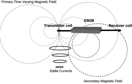
CHAPTER ONE: INTRODUCTION AND LITERATURE REVIEW Fig. 1. 1. Diagram showing the principle of operation of electromagnetic
induction by EM 38 (Geonics Ltd., Mississauga, Ontario,Canada). ...32 CHAPTER TWO: SPATIAL RELATIONSHIPS BETWEEN APPARENT SOIL ELECTRICAL CONDUCTIVITY AND SOIL PROPERTIES:
IMPLICATIONS FOR MANAGEMENT ZONE DELINEATION
Fig. 2. 1. Relationship between humic matter and soil organic matter in the
Kinston field...76 Fig. 2. 2. Kriged field-scale apparent soil electrical conductivity (ECa) maps of (a)
horizontal measurement (ECH) and (b) vertical measurement (ECV) in the
Kinston field...77 Fig. 2. 3. Kriged field-scale apparent soil electrical conductivity (ECa) maps of (a)
horizontal measurement (ECH) and (b) vertical measurement (ECV) in the
Overman field. ...78 Fig. 2. 4. Kriged field-scale apparent soil electrical conductivity (ECa) maps of (a)
horizontal measurement (ECH) and (b) vertical measurement (ECV) in the
Schoolteacher field...79 Fig. 2. 5. Kriged field-scale apparent soil electrical conductivity (ECa) maps of
(a) horizontal measurement (ECH) and (b) vertical measurement (ECV) in the
Baker field...80 Fig. 2. 6. Kriged field-scale apparent soil electrical conductivity (ECa) maps of (a)
horizontal measurement (ECH) and (b) vertical measurement (ECv) in the
Graham field. ...81 Fig. 2. 7. Relationship between vertical apparent soil electrical conductivity (ECa)
and extractable P across three coastal plain and two piedmont fields in North
Carolina...82 Fig. 2. 8. Relationship between vertical apparent soil electrical conductivity (ECa)
and extractable K across three coastal plain and two piedmont fields in North
Carolina...83 Fig. 2. 9. Relationship between vertical measurement of apparent soil electrical
conductivity (ECa) and pH across three coastal plain and two piedmont fields
in North Carolina. ...84 Fig. 2. 10. Relationships between vertical measurement of apparent soil electrical
cation exchange capacity (CEC), and humic matter (HM) within zones
derived from clustering on ECa within each of the five study fields. ...87 Fig. 2. 13. Relationships between zone mean vertical measurement of apparent
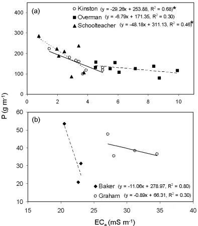
soil electrical conductivity (ECa) and zone mean soil P among zones derived from clustering with ECa across (a) three coastal plain fields and (b) two piedmont fields. Each point represents mean ECa and mean P of a zone. Each regression represents relationship between ECa and extractable P for a field.
Asterisk indicates that relationship is significant at the 0.05 probability level. ...88 Fig. 2. 14. Relationships between zone mean vertical measurement of apparent
soil electrical conductivity (ECa) and zone mean soil K among zones derived from clustering with ECa across (a) three coastal plain fields and (b) two piedmont fields. Each point represents mean ECa and mean K of a zone. Each regression represents relationship between ECa and extractable K for a field. Asterisk indicates that relationship is significant at the 0.05 probability
level...89 Fig. 2. 15. Relationships between zone mean vertical measurement of apparent
soil electrical conductivity (ECa) and zone mean pH among zones derived from clustering with ECa across (a) three coastal plain fields and (b) two piedmont fields. Each point represents mean ECa and mean pH of a zone. Each regression represents relationship between ECa and pH for a field.
Asterisk indicates that relationship is significant at the 0.05 probability level. ...90 Fig. 2. 16. Relationships between zone mean vertical measurement of apparent
soil electrical conductivity (ECa) and zone mean cation exchange capacity (CEC) among zones derived from clustering with ECa across (a) three coastal plain fields and (b) two piedmont fields. Each point represents mean ECa and mean CEC of a zone. Each regression represents relationship between ECa and CEC for a field. Asterisk indicates that relationship is
significant at the 0.05 probability level...91 Fig. 2. 17. Relationships between zone mean vertical measurement of apparent
soil electrical conductivity (ECa) and zone mean humic matter (HM; soil organic matter in the Kinston field) among zones derived from clustering with ECa across (a) three coastal plain fields and (b) two piedmont fields. Each point represents mean ECa and mean HM of a zone. Each regression represents relationship between ECa and HM for a field. Asterisk indicates
that relationship is significant at the 0.05 probability level. ...92 Fig. 2. 18. A scatter plot between vertical measurement of apparent soil electrical
conductivity (ECa) and clay content (0 – 57 cm) in the Kinston field...93 Fig. 2. 19. Relationship between vertical measurement of apparent soil electrical
conductivity (ECa) and clay content (0 – 75 cm) across (a) three coastal plain
fields and two piedmont fields and (b) all five study fields in North Carolina. ...94 Fig. 2. 20. Relationships between zone mean vertical measurement of apparent
mean clay content of a zone. Each regression represents relationship between ECa and clay content at cumulative depths of 0 to 15, 0 to 75, and 0 to 150 cm for a field. Asterisk indicates that the relationship is significant at the
0.05 probability level. ...95 Fig. 2. 21. Overall relationships between mean vertical measurement of apparent
soil electrical conductivity (ECa) and mean clay content (0 – 75 cm) among
zones derived from clustering with ECa across five study fields. ...96
CHAPTER THREE: CHARACTERIZING FIELD-SCALE SOIL ELECTRICAL CONUCTIVITY-SOIL MOISTURE RELATIONS FOR SITE-SPECIFIC
MANAGEMENT
Fig. 3. 1. Sampling locations for soil physical properties, TDR moisture profiling probe locations, and transects of apparent soil electrical conductivity (ECa)
surveys on four days with different naturally occurring soil moisture levels...159 Fig. 3. 2. Mean volumetric soil moisture content at 0- to 15-, 15- to 30-, 30- to 45-,
45- to 60-, and 60- to 75-cm depths on four days with different naturally occurring soil moisture content measured using profiling time domain reflectometry (TDR) probes installed at 60 locations. For this study, the 54 (out of 60) readings that were good for all four surveys were used. Soil moisture contents at field capacity and wilting point were determined in the laboratory using pressure plates with sieved soil samples in equilibrium with a water potential of -33 kPa and -1500 kPa. Mean volumetric soil moisture content within a depth interval followed by the same letter are not
significantly different at α = 0.05...160 Fig. 3. 3. Interpolated maps of soil moisture content (0 – 75 cm) measured on four
days with different naturally occurring soil moisture conditions on which field-scale apparent soil electrical conductivity (ECa) surveys were conducted: (a) 20 March (wet), (b) 13 March (surface dry), (c) 11 August
(subsoil dry), and (d) 15 July (dry). These maps were classified by quantiles...161 Fig. 3. 4. Kriged normalized field-scale apparent soil electrical conductivity (ECa)
maps derived from surveys conducted (a) 20 March (wet condition), (b) 13 March (surface-dry condition), (c) 11 August (subsoil-dry condition), and (d)
15 July (dry condition)...162 Fig. 3. 5. Quantile CV map for apparent soil electrical conductivity (ECa)
measured under four different naturally occurring soil moisture conditions...163 Fig. 3. 6. Nonhierarchical k-means clustering maps derived from (a) 20 March
Fig. 3. 7. The pooled variances ( 2
P
s ) of P, K, pH, CEC, and SOM for (a) clusters derived from apparent soil electrical conductivity (ECa) surveys of four different soil moisture conditions, and (b) clusters derived from ECa surveys with elevation and aerial image near-infrared (NIR) band. Variances were expressed as a percentage of whole field variance ( 2
field whole
s − ). Asterisks below the horizontal axis indicate that 2
P
s values are significantly different from 2
field whole
s − at the 0.05 probability level. The numbers of control zones
are the same as those for zones developed from clustering the data described. ...165
APPENDIX FIGURE B
Fig. B. 1. Interpolated maps of soil moisture contents measured under relatively wet condition (20 March) measured at the individual and cumulative depth
intervals in the Kinston field... 168 Fig. B. 2. Interpolated maps of soil moisture contents measured under relatively
surface dry condition (13 March) measured at the individual and cumulative
depth intervals in the Kinston field... 169 Fig. B. 3. Interpolated maps of soil moisture contents measured under relatively
subsoil dry condition (11 August) measured at the individual and cumulative
depth intervals in the Kinston field... 170 Fig. B. 4. Interpolated maps of soil moisture contents measured under relatively
dry condition (15 July) measured at the individual and cumulative depth
intervals in the Kinston field... 171 Fig. B. 5. Interpolated maps of sand contents measured at the individual and
cumulative depth intervals in the Kinston field. ... 172 Fig. B. 6. Interpolated maps of silt contents measured at the individual and
cumulative depth intervals in the Kinston field. ... 173 Fig. B. 7. Interpolated maps of clay contents measured at the individual and
cumulative depth intervals in the Kinston field. ... 174 Fig. B. 8. Interpolated maps of bulk density measured at the individual and
cumulative depth intervals in the Kinston field. ... 175 Fig. B. 9. Interpolated maps of saturated hydraulic conductivity (Ksat) measured at
the individual and cumulative depth intervals in the Kinston field. ... 176 Fig. B. 10. Interpolated maps of plant available water (water content between -33
kPa and -1500 kPa) measured at the individual and cumulative depth
intervals in the Kinston field... 177 Fig. B. 11. Interpolated maps of cone index measured at the individual and
cumulative depth intervals in the Kinston field. ... 178
Fig. 4. 1. Percentile box plots of soil test P, K, pH, cation exchange capacity (CEC), and humic matter (HM) measured on samples from two coastal plain fields, Kinston (KT) and Overman (OV), and two piedmont fields, Baker
(BK), and Graham (GR). ...227 Fig. 4. 2. Nonhierarchical k-means clustering maps derived from different data
sets in the Kinston field. Each grayscale shade represents a different cluster
(sampling zone); n is the number of clusters (sampling zones) within a field. ...228 Fig. 4. 3. Nonhierarchical k-means clustering maps derived from different data
sets in the Overman field. Each grayscale shade represents a different cluster
(sampling zone); n is the number of clusters (sampling zones) within a field. ...229 Fig. 4. 4. Nonhierarchical k-means clustering maps derived from different data
sets in the Baker field. Each grayscale shade represents a different cluster
(sampling zone); n is the number of clusters (sampling zones) within a field. ...230 Fig. 4. 5. Nonhierarchical k-means clustering maps derived from different data
sets in the Graham field. Each grayscale shade represents a different cluster
(sampling zone); n is the number of clusters (sampling zones) within a field. ...231 Fig. 4. 6. The residual variances ( 2
P
s ) expressed as a percentage of whole field variance ( 2
field whole
s − ) for each management zone derived from clustering with different data sets for (a) P, K, pH, cation exchange capacity (CEC), and soil organic matter (SOM), and (b) crop yields in the Kinston field. An asterisk below the horizontal axis indicates that 2
P
s was significantly different from 2
field whole
s − at the 0.05 probability level. ...232 Fig. 4. 7. The residual variances ( 2
P
s ) expressed as a percentage of whole field variance ( 2
field whole
s − ) for each management zone derived from clustering with different data sets for (a) P, K, pH, cation exchange capacity (CEC), and humic matter (HM), and (b) crop yields in the Overman field. An asterisk below the horizontal axis indicates that 2
P
s was significantly different from 2
field whole
s − at the 0.05 probability level. ...233 Fig. 4. 8. The residual variances ( 2
P
s ) expressed as a percentage of whole field variance ( 2
field whole
s − ) for each management zone derived from clustering with different data sets for (a) P, K, pH, cation exchange capacity (CEC), and humic matter (HM), and (b) crop yields in the Baker field. An asterisk below the horizontal axis indicates that 2
P
s was significantly different from 2
field whole
APPENDIX FIGURE C
Fig. C. 1. Percentile box plots of soil test P measured on samples from the four study fields. Dashed lines indicate probable crop response to fertilization based on soil test levels and the North Carolina Department of Agriculture and Consumer Services (NCDA&CS) Agronomic Division Soil Testing
Laboratory index system...253 Fig. C. 2. Percentile box plots of soil test K measured on samples from the four
study fields. Dashed lines indicate probably crop response to fertilization based on soil test levels and the North Carolina Department of Agriculture and Consumer Services (NCDA&CS) Agronomic Division Soil Testing
CHAPTER ONE
INTRODUCTION
Site-specific management (SSM) has received considerable attention due to the
three main potential benefits of: 1) increasing input efficiency, 2) improving the
economic margins of crop production, and 3) reducing environmental risks. Uniform
management of crops grown under spatially variable conditions can result in less than
optimum yields due to nutrient deficiencies as well as excessive fertilizer application that
may potentially reduce environmental quality (Redulla et al., 1996). Therefore, SSM
requires the development of agronomic strategies to manage spatially variable fields
more efficiently by applying crop inputs in accordance with the specific requirements of
different within-field areas. Recommendation algorithms for varying inputs may be
established assuming a sound understanding of the within-field variability of the soil
chemical and physical properties. Therefore, a study of soil spatial variability necessary
to optimize site-specific soil management in North Carolina should be performed.
In past studies, grid sampling combined with geostatistical analysis has been used
to describe soil spatial variability. However, due to the cost and labor intensity associated
with intensive grid sampling, the concept of management zones has received considerable
attention as a means to improve efficiency and reduce sampling costs. A management
zone is defined as a sub-region of a field that expresses a relatively homogeneous
combination of yield-limiting factors for which a single rate of a specific crop input is
appropriate (Doerge, 1999). Sensor-based information such as remotely sensed data has
shown potential for the development of management zones, because sensor-based
measurements can provide noninvasive, quantitative, and repeatable data reflecting
Apparent soil electrical conductivity (ECa) has become one of the most frequently
used measurements to develop soil and crop management zone strategies due to its
potential correlation with soil properties affecting crop productivity (Johnson et al., 2001;
Schepers et al., 2004). Maps of ECa along with other sensor-based field information such
as landscape attributes and aerial images have been suggested as potential resources for
developing management zones (Fridgen et al., 2004; Schepers et al., 2000; Chang el al.,
2003; Schepers et al, 2004). To use these data for developing management zones, spatial
relationships between these data and variation of soil properties and crop yield in a given
field should be quantified and the factors responsible for that variation identified. We
hypothesize that soil-based management zones using sensor-based data could be
promising tools to improve site-specific crop management in North Carolina. The goal of
our proposed research is to develop strategies for optimal characterization of soil
chemical and physical properties that are important for site-specific soil and crop
management in agricultural fields of the Coastal Plain and Piedmont of North Carolina.
The objectives of this research were to
i) examine the spatial relationships between ECa and soil chemical and
physical properties to determine if ECa could be useful to characterize the
spatial variability of soil properties related to crop productivity to facilitate
ii) evaluate the effects of in-situ soil moisture variation on ECa mapping as a
basis for characterization of soil spatial variability and as a data layer in
cluster analysis as a means of delineating sampling zones.
iii) evaluate clustering approaches using different variable sets for
management zone delineation to characterize the spatial variability of soil
nutrient levels and crop yields in agricultural fields of the Coastal Plain
and Piedmont of North Carolina.
Apparent Soil Electrical Conductivity (ECa)
Apparent soil electrical conductivity (ECa) has become one of the most frequently
used measurements to characterize field variability for application to site-specific
management (SSM) due to its relative ease of use and its potential correlation with soil
characteristics that can affect crop productivity. In fact, ECa has no direct effect on crop
growth and yield, but the spatial variation of ECa has been shown to be correlated with
soil properties affecting crop productivity. Several studies have reported thatECa is
related to variation in crop productivity caused by soil differences(Jaynes et al., 1995;
Kitchen et al., 1999; Luchiari et al., 2001). In general, ECa can be affected by anumber
of different soil properties, including soil water content (Kachanoski et al., 1988;
Kachanoski et al., 1990;), soil organic matter (Jaynes et al., 1995; Banton et al., 1997),
drainage conditions (Kravchenko et al. 2002), salinity (Williams and Hoey, 1987;
McNeill, 1992), soil texture (Williams and Hoey, 1987; Banton et al., 1997), and depth to
on some soils as a surrogate measureof soil chemical and physical properties at low cost
(Jaynes, 1996;Clark et al., 2001; Hartsock et al., 2001).
It is important to understand the basic theories and principles of ECa measurement
to appreciate their application in characterizing soil spatial variability for site-specific soil
and crop management. The electrical conductivity model suggested by Rhoades et al.
(1989) indicate that ECa measurement is a function of soil physical and chemical
properties such as soil salinity, saturation percentage, soil moisture content, and soil bulk
density. Using equations [1]-[6] formulated by Rhoades et al. (1989), the ECa can be
estimated: W SW W SS SS SW SS a
EC
EC
EC
=
(
+
)
×
+
(
−
)
×
2
θ
θ
θ
θ
θ
[1] 100 ) ( b W PW ρθ = × [2]
011 . 0 639 . 0 + = W SW θ
θ [3]
65 . 2 b SS ρ
θ = [4]
434ECSS =0.019(SP)−0. [5]
ECe = electrical conductivity of saturation extracts (dS m-1)
θSS = volumetric water content in the soil-solid pathway (cm3 cm-3)
θSW: = volumetric water content in the soil-water pathway (cm3 cm-3)
θw = total volumetric water content (cm3 cm-3)
SP = saturation percentage
PW = soil gravimetric water content (g cm-3)
ρb = soil bulk density (g cm-3).
Since soil bulk density and saturation percentage are closely associated with the soil
texture and soil moisture, ECa measurements in non-saline soils could be driven primarily
by soil texture and soil moisture (Corwin and Lesch, 2003). Both soil texture and soil
moisture are primary controlling factors affecting soil water availability to crops. Because
soil water is one of the essential factors that affect yield variation, ECa maps often exhibit
similar spatial patterns to yield maps. Therefore, spatial measurement of ECa has been
examined as a potential measurement for explaining variability in crop productivity.
Currently, there are two primary methods of measuring ECa, the direct or contact
method and a non-contact method that utilizes electromagnetic induction (EMI). Contact
methods use voltage between electrodes in contact with the soil, directly measure the
resistance of the soil to the resulting current, the reciprocal of which is a direct measure
of ECa. The principle of electromagnetic induction used to measure ECa is shown in Fig.
1.1 (Rhoades et al., 1989). A radio frequency transmitter coil generates primary
time-varying magnetic fields. These magnetic fields induce circular eddy-current loops in the
soil in the area surrounding that loop. Each current loop generates a secondary
electromagnetic field that is proportional to the value of the current flowing within the
loop. A receiver coil in the vicinity of the transmitter coil intercepts a portion of the
electromagnetic field from each loop and through the instrument circuitry and appropriate
functions, a measurement of ECa is derived.
Rapid spatial measurement ofECa can be accomplished using non-contact EMI
sensors (McNeil, 1992)or direct-contact sensors such as rolling coultersthat measure
electrical resistance directly (Lund et al., 1999). The EM38 (Geonics Limited,
Mississauga, Ontario, Canada) is a non-invasive sensor that uses the principle of EMI to
measure ECa. The EM38 is a lightweight bar designed to be carried byhand and provide
stationary ECa readings. The EM38 is designed specifically for measuring ECa in the
surface 0 to 0.75 m of soil in the horizontal mode and from 0- to 1.5-m depth in the
vertical mode. This is approximately the same depth as the rooting zone of annual crops.
Sensitivity to the near surfacein the vertical dipole mode is relatively low but increases
with depth, with maximum sensitivity at about 30 to 60 cm. Inthe horizontal dipole
mode, sensitivity is at a maximum at thesurface and decreases exponentially with depth
(McNeil, 1992; McKenzie et al., 1989). The other popular ECa sensor, the Veris Model
3100 sensor cart (Veris Technology, Salina, Kansas), identifies soil variability by directly
sensing ECa. As the Veris 3100 cart is pulled through the field, a pair of coulter
EMI and direct sensing methods. Maps generated from the two sensors exhibited similar
patterns at the field scale. Differences between maps were attributed to variations in
sensing depth between the two sensors.
Management Zones
The concept of management zones has been proposed as a solution to the
problems associated with grid sampling as well as a method to more efficiently apply
crop inputs in site-specific management (SSM). The delineation of management zones is
a way of classifying the spatial variability within a field into subregions with similar soil
properties and crop growth parameters, where a uniform rate of a particular crop input is
appropriate (Doerge, 1999). The basic idea of management zones is that fields can be
sampled using a zone or directed sampling method where soil samples are composited
from field subregions (zones) similar input use efficiency, crop yield potential, or
environmental impacts (Pocknee et al., 1996). Each management zone can be
characterized via the minimal amount of sampling required to describe soil characteristics
within it. Therefore, zone sampling can minimize the number of soil samples necessary
for field characterization compared to intensive grid sampling.
To attain maximum efficiency of crop inputs through a management zone strategy,
the following practical considerations for defining management zones were suggested by
Doerge (1999): a relationship with crop yield, free or low cost of data, data that are
quantitative and repeatable, high density of the data, and scale of the data appropriate to
the variable rate management anticipated. Therefore, remote sensing technology is
cost-quantitative data. Additionally, scientific evidence supporting the practical useof remote
sensing technology to characterize soil characteristics important to management is
increasing (Varvel et al., 1999).
A number of procedures have been used to identify within-field management
zones for site-specific management (SSM). The potential resources for the field
characteristics commonly used to define management zones are management history,
aerial images, terrain attributes, yield maps, soil surveys, and sensors for detecting soil
property information (e.g., electrical conductivity) (Doerge, 1999). For example, one
approach uses relatively stable soil properties such as ECa and/or landscape features in
conjunction with soil-landscape models to estimate patterns of soil variability (Bell et al,
1995). Topographic attributes and landscape position data have been widely used to map
within-field areas of high and low productivity based on water availability (Jones et al.,
1989; Jaynes et al., 1995; Sudduth et al., 1997). In these studies, footslope positions
generally out-yielded side-slope positions unless ponding resulted from poor drainage.
Spatial measurements of ECa have also been used to delineate management zones based
on yield variability caused by soil water differences (Jaynes et al., 1995; Sudduth et al.,
1995). Fraisse et al. (1999) showed that ECa, elevation, and slope were the most useful
attributes for the delineation of within-field management zones. Franzen et al. (2000)
determined that zones based on topography significantly reduced the amount of sampling
Higher yields were associated with higher SOM and the yield differences between each
management zone were statistically significant.
An alternative source of high spatial resolution information that has been used in
the development of potential management zones is image-based remote sensing. Fleming
et al. (2004) used aerial images of soil color, topography, and farmers’ management
experience to delineate MZ in two irrigated Iowa cornfields. Bare-soil images along with
elevation, aspect, slope, and soil electrical conductivity have been applied to delineate
soil-based management zones (Blackmer and Schepers, 1996; McCann et al., 1996;
Fleming el al., 2004; Gerwig el al., 2000; Luchiari et al., 2001; Schepers et al., 2000).
Multi-year yield maps have been used to develop yield zones. Researchers have
begun to examine the patterns observed in yield maps, based on the premise that crop
yield variation is affected by soil spatial variability (Boydell and McBratney, 1999;
Flowers et al., 2005). Kitchen et al. (1995) used a classified yield map from the previous
year to determine “yield potential” zones within a field. Their success was quantified by
applying variable N fertilizer according to yield goals calculated for each zone, and
observing a reduction in residual soil nitrate (NO3) in comparison with uniform treatment
within the zones. When more than one year’s yield maps are available for a field, the
recognition of stable response patterns becomes important for the determination of
management units. Van Uffelen et al. (1997) proposed a weighted taxonomic distance
measure to quantify the similarity between patterns in yield maps over 8 years of
simulated data. A benefit of the simulation process is that yield levels displayed in the
dominant pattern may be utilized as the yield goals for the management units. Lark and
analysis on three years yield data in an attempt to define regions of a field that may
present similar factors limiting/governing yield.
Landscape Attributes Related to Yields and Soil Properties
Landscape attributes have been shown to be a critical factor affecting yield
variability. Since plant-available water and soil physical and chemical properties vary
with landscape position and contribute to differences in plant response and yields,
landscape attributes have shown a potential to explain yield variability in previous studies.
Wibawa et al. (1993) found that yield potentials were different depending on landscape
positions. Higher corn yields were found on footslopes than backslopes, which had
higher yields than summit positions. Relationships between spatial variability of field
parameters and corn yield variation were evaluated by Karlen et al. (1999). They
reported that the corn yield variation was correlated with landscape attributes. Khakural
et al. (1999) also found that landscape position was related to soybean and corn yields.
Nolan et al. (1995) reported that landscape position was related to yield increases due to
fertilizer additions in an Alberta field. They found that wheat and canola yield responses
due to N fertilizer additions were greater on footslope positions than on shoulderslope
positions. Yield differences were primarily influenced by differences in nutrient
efficiency related to soil available water. Fiez et al. (1994) found that landscape position
landscape position varied depending on fields in Minnesota. Wyciskalla et al. (2000)
also reported that landscape attributes were correlated to soil chemical and physical
properties, but not to corn yield in the Illinois fields.
Previous studies have also showed correlations between landscape attributes and
soil chemical and physical properties. Brubaker et al. (1993) also reported that soil
properties varied with landscape position in eastern Nebraska fields. Extractable K, CEC,
clay content, and soil organic matter generally decreased down slope, while sand and silt
contents, pH, extractable Ca and Mg, and base saturation (BS) generally increased down
slope. Khakural et al. (1996) reported that landscape attributes were correlated with
nutrient levels and soil texture in glacial soils. Pachepsky et al. (2001) found that slope
derived from a digital elevation model (DEM) was correlated to soil texture. They
reported that 60% of the variation in soil water content, which was correlated to soil
texture, was explained by landscape attributes.
The potential relationship of landscape attributes with soil properties and crop
yields observed in these studies suggests that landscape properties could be essential
information for SSM, especially for developing management zones.
Aerial Soil Imagery in SSM
Remotely sensed images have been proposed as auxiliary attributes for directed
sampling for SSM (Bhatti et al., 1991; Mulla, 1997; McCann et al., 1996; Franzen et al.,
1999). Optical remote sensing technology offers the potential for identifying fine-scale
spatial patterns in soil properties and crop yield within fields, and optimizing the soil
Remote sensing provides three major types of imagery: aerial photography,
airborne imagery from video and digital cameras, and satellite imagery. Aircraft-based
remote sensing can provide valuable information for SSM application because of its
ability to acquire timely high resolution imagery over an entire field or even a larger area
during the growing season. Therefore, images from aircraft-based sensors have a unique
role for monitoring seasonally variable soil and crop conditions and for time-specific and
time-critical crop management. Among the advantages of airborne imagery are its low
cost, real-time or near-real-time availability of imagery for visual assessment and
computer image processing, and its ability to obtain high spatial resolution spectral data
in the visible to mid-infrared region of the spectrum (Everitt and Escobar, 1989; Mausel
et al., 1992; Everitt et al., 1995). Therefore, it has been used in precision agriculture for
study of soil and crop conditions (Blackmer and White, 1996; Tomer et al., 1997). Digital
aerial and satellite remote sensing technology allows detailed information on a 1 m scale
to be collected across a field. Despite the current evolution of ever more sophisticated
digital imaging systems, aerial film photography remains one of the most reliable and
most widely used forms of remotely sensed imagery. Airborne imagery from both video
and digital cameras is a fairly new remote sensing technique. It has been used as a
versatile data-gathering tool for assessing natural resources and monitoring agricultural
crops since the 1980s (Everitt and Nixon, 1985; Pearson et al.,1994). Current satellite
For SSM, there are specific requirements on the spatial, spectral, and temporal
resolutions of remotely sensed imagery. Since precision farming requires detailed
information about soil and crop conditions, a spatial resolution of 5 m or less seems to be
required and some specific applications may need resolutions in the order of centimeters
(Robert, 1996). Timeliness is also a very important requirement for using remote sensing
data in some agricultural applications. Some applications such as crop stress, disease, and
pest management may require information within a few hours to a few days of when the
problems occur, while others may require information at regular intervals over the
growing season. Moreover, the frequency of image acquisition needs to be flexible to
account for cloud interference. Airborne video and digital imagery can meet most of the
spatial, spectral, and temporal requirements for SSM.
Soil color can provide information about surface soil conditions such as soil
moisture and organic matter for site-specific management practices (Schepers and
Blackmer, 1996). Black and white images effectively display surface soil organic matter
that can be correlated to soil texture and landscape position. The advantage of aerial
photographs is that they are easily obtained, cover a large area, and are relatively
inexpensive. McCann et al. (1996) determined that black and white aerial photographs
could be used as a cost-effective method to delineate soil management units. In a glacial
till soil in Saskatchewan, management units made from the photographs had a close
relationship to intensively measured soil properties related to soil organic matter. Mulla
et al. (2000) found that targeted sampling utilizing near infrared (NIR) images of bare
soil and crop canopies resulted in significant savings over uniform rate lime applications.
conditions and during the cropping season to identify the variability of soil texture, weed
levels, and soil P levels. Results were used to subdivide two fields with high spatial
variability into management zones. Yang and Anderson (1999) delineated management
zones by classifying aerial CIR digital video images of grain sorghum fields into zones of
homogeneous spectral response using an unsupervised classification procedure. Spectral
responses in the green, red, and near infrared (NIR) portions of the spectrum were used to
estimate biomass, leaf area index (LAI), and crop yield. Grain yields were found to be
significantly different among the production zones.
Cluster Analysis
Cluster analysis has been one of the most frequently used computational methods
to develop soil and crop management zones (Fridgen et al., 2004; Schepers et al., 2000;
Chang el al., 2003; Schepers et al, 2004). Since the primary objective of cluster analysis
is to define the structure of the data by placing the most similar observations into groups,
cluster analysis is appropriate to delineate management zones.
Cluster analysis is generally characterized as a descriptive, atheoretical, and
noninferential method. Since cluster analysis has no statistical basis upon which to draw
statistical inferences from a sample to a population, it is used primarily as an explanatory
technique. Therefore, clustering solutions may not be unique, as the cluster membership
1998), resulting in different management zones for a given field. The selection of
relevant variables for cluster analysis could be critical to attain maximum efficiency of
management zone strategy.
Nonhierarchical k-means clustering is commonly used to group data into naturally
occurring clusters aiming to minimize within-cluster variance and maximize
between-cluster variance (Khattree and Naik, 2000). Cluster analysis uses the measurement of
“distances” between observations to group the observations. The Mahalanobis distance,
a standardized form of the Euclidean distance, is most frequently used to measure
dissimilarity (Khattree and Naik, 2000). The Mahalanobis distance approach performs a
standardization process on the data by scaling in terms of the standard deviations and also
sums the pooled within-group variance-covariance, which adjusts intercorrelations
among the variables. The Mahalanobis distance is defined as:
) ( ) ( ) , ( 1 b a S b a b a
d = − ′ − −
where S–1 is the inverseof the pooled sample variance-covariance matrix, and a and b are
the respective vectorsof measurements on groups 1 and 2. This measure has the distinct
advantage of accounting for any correlations that might existbetween the variables.
Nonhierarchical k-means cluster analysis using SAS PROC FASTCLUS involves
three basic steps (Khattree and Naik, 2000). First, the seedsas the initial centroids for the
k clusters are selected using least squares. Second, all observations are assigned to the
respectiveclusters with the nearest seed. All cluster seeds are updated by replacing old
become very small or zero. Finally,when all observations are assigned to the clusters
with seedsnearest to the corresponding observations, the final clustersresult.
One important problem in clustering analysis is to determine the number of
clusters in a given data structure. A goodness-of-fit criterion such as R2 can only be
utilized when the sampling distribution of the criterion to enable tests of cluster
significance is known. Therefore, ordinary significance tests, such as analysis of
variance F tests, are not valid for testing differences between clusters. Since clustering
methods attempt to maximize the separation between clusters, the assumption of random
samples for the usual significance tests, parametric or nonparametric, are violated.
The cubic clustering criterion (CCC) (Sarle, 1983) has commonly been used to
estimate the number of clusters developed from Ward's minimum variance method,
k-means, or other methods based on minimizing the within-cluster sum of squares. The
CCC is based on the assumption that clusters are obtained from a uniform distribution on
a hyperbox or hypercubes of the same size. The first step in devising a valid significance
test for clusters is to specify the null and alternative hypotheses:
H0: the data have been sampled from a uniform distribution on a hyperbox.
Ha: the data have been sampled from a mixture of spherical multivariate normal
and
where R2 represents the proportion of variance explained by clusters. E(R2) is its
expected value under the null hypothesis, and p is an estimate of dimensionality of the
between-cluster variation. Positive values of the CCC mean that the obtained R2 is greater
than would be expected if sampling from a uniform distribution and therefore indicate the
possible presence of clusters. A good clustering is indicated by CCC >3. Higher values of
CCC indicate better clustering. If CCC continues to increase with the number of clusters,
it may indicate that the observations within a cluster are forming the pockets of several
subclusters. The number of clusters in a given data structure is determined by the cubic
clustering criterion (CCC), which is obtained from a uniform distribution on a hyperbox
or hypercubes of the same size. The performance of the CCC is evaluated by Monte
SUMMARY
Numerous studies have investigated the potential use of ECa to describe soil
spatial variability at the field scale and to develop management zones for application to
site-specific management (SSM). Spatial measurements of ECacan be used on some soils
as a surrogate measureof soil chemical and physical properties related to crop yield at
low cost for SSM (Jaynes, 1996;Clark et al., 2001; Hartsock et al., 2001). Therefore, ECa
mapping has been used to characterize soil spatial variability for soil sampling design
(Johnson et al., 2001) and as a data layer for developing soil-based management zones
(Chang el al., 2003; Fleming et al, 2004; Schepers et al., 2004). Cluster analysis of
sensor-based field attributes such as ECa, bare soil radiance as captured by aerial
photography, and terrain attributes such as elevation and slope has been widely applied to
delineate soil and crop management zones (Chang el al., 2003; Fridgen et al., 2004;
Schepers et al, 2004).
In a previous study (Heiniger et al., 2003), ECa was evaluated as a means to
estimate plant nutrient concentrations in North Carolina soils. This study indicated that it
was unlikely that ECa could be used to directly estimate soil nutrient content in a field.
However, the authors suggested that additional research on the relationships of ECa with
soil moisture and soil texture would be necessary to determine whether ECa could be
between ECa and soil chemical and physical properties to determine if ECa could be
useful in characterizing soil properties related to crop productivity and thus useful for
SSM, (ii) the effects of in-situ soil moisture variation on ECa mapping as a basis for
characterization of soil spatial variability and as a data layer in cluster analysis to
delineate sampling zones, and (iii) clustering approaches using different data sets for
management zone delineation to minimize spatial variability in soil nutrient levels and
crop yields in agricultural fields of the Coastal Plain and Piedmont of North Carolina.
This information could be essential for the successful utilization of ECa sensors as well as
REFERENCES
Banton, O., M.K. Seguin, and M.A. Cimon. 1997. Mapping field-scale physical
properties of soil with electrical resistivity. Soil Sci. Soc. of Am. J. 61:1010-1017.
Bell, J.C., C.A. Butler, and J.A. Thompson. 1995. Soil-terrain modeling for site-specific
agricultural management. p. 209-227. In P.C. Robert et al (ed.) Proc. Int. Conf.
Site-Specific Manage. Agric. Syst., 2nd, Minneapolis, Mn, 27-30 March 1995.
ASA, CSSA, and SSSA, Madison, WI.
Bhatti, A.U., D.J. Mulla, and B.E. Frazier. 1991. Estimation of soil properties and wheat
yields on complex eroded hills using geostatistics and Thematic Mapper images.
Remote Sens. Environ. 37:181-191.
Blackmer, T.M. and J.S. Schepers. 1996. Aerial photography as an aid in soil sampling.
Better-Crops-with-Plant-Food. 80 (3): 18-19.
Blackmer A.M. and S.E. White. 1996. Remote sensing to identify spatial patterns in
optimal rates of nitrogen fertilization. p. 33-43. In P.C. Robert et al. (ed.) Proc.
Int. Conf. Precision Agric.,3rd, Minneapolis, MN. 23-26 June 1996.
ASA-CSSA-SSSA, Madison, WI
Boydell B. and A.B. McBratney, 1999. Identifying potential within-field management
zones from cotton yield estimates. p. 331-341. In J.V. Stafford (ed.) Proc. Eur.
Bruulsema, T.W., G.L. Malzer, P.C. Robert, J.G. Davis, and P.J. Copeland.1996. Spatial
relationships of soil nitrogen with corn yield response to applied nitrogen. p.
505-512. In P.C. Robert, et al. (ed.) Proc. Int.. Conf. Precision Agric., 3rd, Minneapolis,
MN. 23-26 June 1996. ASA, CSSA, SSSA. Madison, WI.
Chang, J., D.E. Clay, C.G. Carlson, S.A. Clay, D.D. Malo, R. Berg, J. Kleinjan, and W.
Weibold. 2003. Different techniques to identify management zones impact
nitrogen and phosphorous sampling variability. Agron. J. 95:1550-1559.
Clark, R.L., F. Chen, D.E. Kissel, and W. Adkins. 2001. Mapping soil hardpans with the
penetrometer and electrical conductivity. In P.C. Robert et al. (ed.). Proc. Int.
Conf. Precision Agric., 5th, Minneapolis, MN. 16–19 July 2000. ASA, CSSA, and
SSSA, Madison, WI.
Corwin, D.L., and S.M. Lesch. 2003. Application of soil electrical conductivity to
precision agriculture: Theory, principles, and guidelines. Agron. J. 95:445-471.
Doerge, T.A.. 1999. Management zone concepts. In Site-specific management guidelines.
Potash and Phosphate Institute, Atlanta,GA.
Doolittle, J.A., K.A. Sudduth, N.R. Kitchen, and S.J. Indorante. 1994. Estimating depths
to claypans using electromagnetic induction methods. J. Soil and Water Cons.
49:572-575.
Everitt, J.H., and D.E. Escobar. 1989. The status of video systems for remote sensing
applications. p. 6-29. In Proc. Biennial Workshop on Color Photography and
Videography in the Plant Sciences and Related Fields, 12th, American Society for
Everitt, J.H., D.E. Escobar, I. Cavazos, J.R. Noriega, and M.R. Davis. 1995. A
three-camera multispectral digital video imaging system. Remote Sens. Environ.
54:333-337.
Everitt, J.H. and P.R. Nixon. 1985. Video imagery: a new remote sensing tool for range
management. J. Range Manage. 38 :42l-424.
Fiez, T.E., B.C. Miller, and W.L. Pan. 1994. Winter wheat yield and grain protein across
varied landscape positions. Agron. J. 86:1026-1032.
Fiez, T.E., W.L. Pan, and B.C. Miller. 1995. Nitrogen use efficiency of winter wheat
among landscape positions. Soil Sci. Soc. Am. J. 59:1666-1671.
Fleming, K.L., D.F. Heermann, and D.G. Westfall. 2004. Evaluating soil color with
farmer input and apparent soil electrical conductivity for management zone
delineation. Agron. J. 96:1581-1587.
Flowers, M., R. Weisz, and J.G. White. 2005. Yield-based management zones and grid
sampling strategies: Describing soil test and nutrient variability. Agron. J. 97:
968-982.
Fraisse, C.W., K.A. Sudduth, N.R. Kitchen, and J.J. Fridgen. 1999. Use of unsupervised
clustering algorithms for delineating within-field management zones. Paper No.
993043, ASAE, Toronto, Ontario, Canada, 18-21 July 1999.
Franzen, D.W., A.D. Halvorson, and V.L. Hofman. 2000. Management zones for soil N
Franzen, D.W., L. Reitmeier, J.F. Giles, and A.C. Cattanach. 1999. Aerial photography
and satellite imagery to detect deep soil nitrogen levels in potato and sugarbeet. p.
281-290. In P.C. Robert et al. (ed.) Proc. Int. Conf. Precision Agric., 4th, St. Paul,
MN. 19-22 July, 1998. ASA-CSSA-SSSA. Madison, WI.
Fridgen, J.J., N.R. Kitchen, K.A. Sudduth, S.T. Drummond, W.J. Weibold, C.W. Fraisse.
2004. Management zone analyst (MZA): Software for subfield management zone
delineation. Agron. J. 96:100-108.
Gerwig, B.K., Sadler, E.J., and Evans, D.E. 2000. Evaluating techniques for defining
management zones in the SE Coastal Plain. p. 1-13. In P.C. Robert et al. (ed.)
Proc. Int. Conf. on Precision Agric., 5th, Bloomington, MN. 16-19 July 2000.
ASA-CSSA-SSSA, Madison, WI.
Hair J.F., R.E. Anderson, R.L. Tatham, and W.C. Black. 1998. Multivariate data analysis.
5th ed. Prentice-Hall, Inc. Upper Saddle River, NJ.
Hartsock, N.J., T.G. Mueller, G.W. Thomas, R.I. Barnhisel, K.L. Wells, and S.A. Shearer.
2001. Soil electrical conductivity variability. In P.C. Robert et al. (ed.) Proc. Int.
Conf. on Precision Agric., 5th, Bloomington, MN. 16–19 July 2000. ASA, CSSA,
and SSSA, Madison, WI.
Heiniger R.W., R.G. McBride, and D.E. Clay. 2003. Using soil electrical conductivity to
improve nutrient management. Agron. J. 95: 508-519.
Jaynes, D.B. 1996. Improved soil mapping using electromagnetic induction surveys. p.
169–179. In P.C. Robert et al. (ed.) Proc. Int. Conf. Precision. Agric., 3rd,