A Thesis Submitted for the Degree of PhD at the University of Warwick
http://go.warwick.ac.uk/wrap/71000
This thesis is made available online and is protected by original copyright. Please scroll down to view the document itself.
Interactions between riverbed morphology,
water chemistry and microbial diversity; and
its impact on pollutant biodegradation
by
Andrew Giuseppe King, MSc, Bsc (Hons)
This thesis is submitted for the degree of
Doctor of Philosophy
School of Life Sciences, University of Warwick, Coventry, UK
Table of Contents
Table of Contents………... i
List of Tables………... viii
List of Figures………... ix
Glossary of Terms………... xxi
Acknowledgements………... xxii
Declaration………... xxv
Abstract………... xxvi
Chapter 1……….………...1
1.1 Introduction………...1
1.2 Down the drain chemicals……….3
1.2.1 Pathways of entry of Down the Drain Chemicals into the environment……….4
1.3 Consequences of chemical release into the environment………...5
1.4 Regulatory drivers for chemical management………...6
1.5 Determination of Biodegradation Rates………..7
1.5.1 Predictive Modelling………...8
1.5.2 OECD testing………..8
1.5.3 Overview of current testing………...9
1.5.3.1 Ready Biodegradability Tests………...9
1.5.3.2 Inherent biodegradation tests………...9
1.5.3.3 Simulation tests………....10
1.6 Environmental Realism of testing………..10
1.6.1 Effect of environmental factors on biodegradability assessment………...11
1.6.2 Water Chemistry………..12
1.6.3 Inoculum………14
1.6.3.1 Biofilm as Inoculum………..15
1.7 Hyporheic exchange………16
1.7.1 Solute transport………18
1.7.2 Diffusion……….18
1.7.2.1 Molecular Diffusion………..19
1.7.2.2 Effective Diffusion……….19
1.7.3 Pumping……….20
1.7.4.1 In-situ testing……….23
1.7.4.2 Ex-situ testing………24
1.7.5 Predictive scaling relationships………..24
1.8 Biofilms………..25
1.9 Study Objectives………..28
Chapter 2………..30
2.1 Introduction………30
2.2 Materials and Methods………32
2.2.1 Experimental Rig………..32
2.2.1.1 Materials………35
2.2.1.2 Pump/Mechanical components of system…………35
2.2.1.3 Sediment………37
2.2.1.4 Study Site………..38
2.2.1.5 Uniform Flow ………40
2.2.2 Fluorometry ………..41
2.2.2.1 Tracer Selection………41
2.2.2.2 Instrumentation……….42
2.2.3 Experimental Development……….45
2.2.3.2 High temperature re-circulation………..45
2.2.3.3 Temperature Compensation………...47
2.2.4 Tracer Decay ………47
2.2.5 Consecutive Dosing……….50
2.2.6 Sinusoidal oscillations……….50
2.2.7 Flow Depth………54
2.3 Functional Schematic………..55
2.3.1 Defined Parameters………...………..55
2.3.2 Example Trace Test………...………….……56
2.3.3 Analytical Development………...…………57
2.3.3.1 Established analysis………57
2.3.3.2 Analysis using GenStat………...61
2.3.3.2.1 Reduction of scatter: Smoothing……….61
2.3.3.2.2 Gradient Identification………63
2.4 Results………..….……65
2.4.1 Temperature Compensation………..…….……65
2.4.2 Rhodamine Concentration Decay……….….…67
2.4.3 Consecutive Dosing……….………70
2.4.4 Sinusoidal Oscillations……….………72
Chapter 3………..…76
3.1 Introduction………76
3.1.1 Hyporheic Exchange………78
3.1.1.1 Solute Transport………...………79
3.1.1.2 Molecular Diffusion………..79
3.1.1.3 Effective Diffusion……….79
3.1.1.4 Predicting Scaling Relationships………80
3.1.1.5 Hyporheic Exchange Tests……….83
3.1.2 Impact of biofilms on exchange……….85
3.1.2.1 Sediment Clogging……….…………..87
3.2 Objectives………..88
3.3 Methods……….89
3.3.1 Determine effect of sediment particle size on the rate of exchange in an experimental flume……….………..90
3.3.1.1 Experimental Apparatus………..90
3.3.1.2 Experimental Design………92
3.3.2 Elucidate the difference in rate of exchange between flat and undulating beds in the flume systems………...94
3.3.2.1 Experimental Apparatus………..94
3.3.2.2 Experimental Design………95
3.3.3 Determine how sediment particle size affects biofilm development ……….96
3.3.3.1 Water Collection Site………...96
3.3.3.2 Experimental Set Up………96
3.3.4 Quantify the impact of biofilm on the rate of exchange as a result
of clogging of interstitial pore spaces in flat bed systems………..99
3.3.4.1 Sampling Procedure and Techniques………...99
3.3.4.2 Experimental Set Up………...……….99
3.3.4.2.1 Hyporheic Exchange Tests……….99
3.3.4.2.2 Microbial Community Surface Development………...100
3.3.4.2.3 Microbial Community Depth Penetration……….………101
3.3.4.2.4 Water Chemistry Tests………..103
3.3.4.3 Trace Data Analytical Techniques………..103
3.3.5 Identify whether the wavelength of dunes affects biofilm development and hyporheic exchange………...104
3.3.5.1 Sampling Procedure and Techniques……….104
3.3.5.2 Experimental Design……….104
3.3.6 Statistical Analysis ………106
3.3.6.1 Analysis of hyporheic exchange rates………106
3.3.6.2 Statistical analysis of total carbohydrate data…...107
3.3.6.3 Biofilm and Water Chemistry Analysis……..…….107
3.4 Results……….108
3.4.1 Impact of sediment particle size on hyporheic exchange………108
3.4.2 Impact of bed-form morphology on hyporheic exchange………109
3.4.3 Microbial development on different sediment particles sizes…..110
3.4.5 Effect of particle size and microbial development on hyporheic
exchange in flat bed re-circulating flume systems………116
3.4.6 Impact of bed-form wavelength on microbial development and its subsequent effect on hyporheic exchange………116
3.5 Discussion……….………..………129
3.5.1 Effect of Sediment Size on Hyporheic Exchange in Experimental System………..……..……….129
3.5.2 Effect of Bed-Form on Hyporheic Exchange in Experimental System……….……..……….…….130
3.5.3 Effective Depth Penetration of Microbial Community on Differing Sediment Particle Sizes………131
3.5.4 Impact of Microbial Development on Hyporheic Exchange…….132
3.5.4.1 Microbial Community Development on Different Sediment Particle Sizes in Flat-Bed Experimental system………..132
3.5.4.2 Impact of Microbial Community on Hyporheic Exchange in Flat Bed System………...………...134
3.5.4.3 Microbial Community Development on Different Sediment Particle Sizes in Undulating-Bed Experimental system……….135
3.5.4.4 Impact of Microbial Community on Hyporheic Exchange in Flat Bed System...137
Chapter 4………140
4.1 Introduction………...140
4.1.1.1 OECD Tests………141
4.1.1.2 Factors that could enhance the realism of OECD tests outcome ………...141
4.1.1.2.1 Light……….………142
4.1.1.2.2 Spatial variability of degradation rates in aquatic systems...143
4.1.1.2.3 Chemical concentration…….144
4.1.1.2.4 Para-Nitrophenol………145
4.2 Objectives………...146
4.3 Methods………..147
4.3.1 Identify the relative roles of different river sediments and water for PNP degradation in aquatic systems……….……147
4.3.1.1 Sample Collection……….147
4.3.1.2 Sample Collection Site……….148
4.3.1.3 Experimental set up………..149
4.3.1.4 Measurement of PNP biodegradation…………...151
4.3.2 Determine the impact of light and dark conditions on the rate of PNP degradation………...152
4.3.2.1 Sample Collection………...152
4.3.2.2 Sample Collection Site………..152
4.3.2.3 Experimental set up………...153
4.3.2.4 Measurement of PNP biodegradation………154
4.3.2.5 Measurement of Chlorophyll-a………....154
4.3.3.1 Sample Collection………..156 4.3.3.2 Sample Collection Site………..156 4.3.3.3 Experimental set up………...158 4.3.3.4 Measurement of PNP biodegradation…………....159 4.3.4 Statistical analysis………...159
4.3.4.1 Analysis of HPLC degradation rates………...159 4.3.4.2 Statistical analysis of PLFA and soil sediment composition……….159 4.4 Results………...160 4.4.1 Impact of river sediment and water for PNP degradation in aquatic systems………...160 4.4.2 Impact of light and dark conditions on the rate of PNP
degradation………...161 4.4.3 Variance in different river sediments and water for PNP
degradation in aquatic systems………...166
4.5 Discussion………...170
4.5.1 Relative roles of river sediment and water for PNP degradation in aquatic systems………...170
4.5.2 Impact of light and dark conditions on the rate of PNP
degradation………...172
Chapter 5 General Discussion………...177
5.1 Reproducibility and Functionality of Experimental System……...177
5.2 Interactions between bed morphology, sediment particle size, biofilm development and hyporheic exchange in re-circulating flume systems………...179
5.3 Assessment of the transformation rate of p-nitrophenol in aquatic sediment systems; utilizing inter sample comparison to evaluate spatial variability of chemical degradation rates………...182
5.4 Impact of Sediment Composition on Experimental Research…………184
5.5 Future Recommendations ………...185
5.6 Future Work………...186
5.7 Project Summary………...189
References………....196
List of Tables
Table 2.1: Glass bead Flume Test Experimental Parameters...49
Table 2.2: Expected and Recorded End Concentrations at each
Consecutive Dose...71 Table 3.1: Experimental parameters utilized by O’Connor and
Harvey (2008)...82 Table 3.2: Comparison of biofilm development on different sized glass beads at depth in a closed, ex-situ system………...112 Table 3.3: Comparison of the amount of the surface area of carbohydrate on
different sized sediments………..112 Table 4.1: Mean biodegradation rates of PNP recorded from experimental
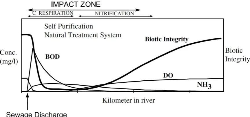
List of Figures
Figure 1.1: Relationship of impact zone caused by direct discharge of organic
wastes...13
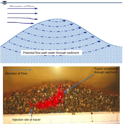
Figure 1.2: Schematic example of potential pumping movement through a bed-form compared against an enhanced experimental tracer photograph of a similar bed-form, illustrating the tracer movement through the bed via pumping...22
Figure 1.3: Illustration describing stages involved in biofilm formation...26
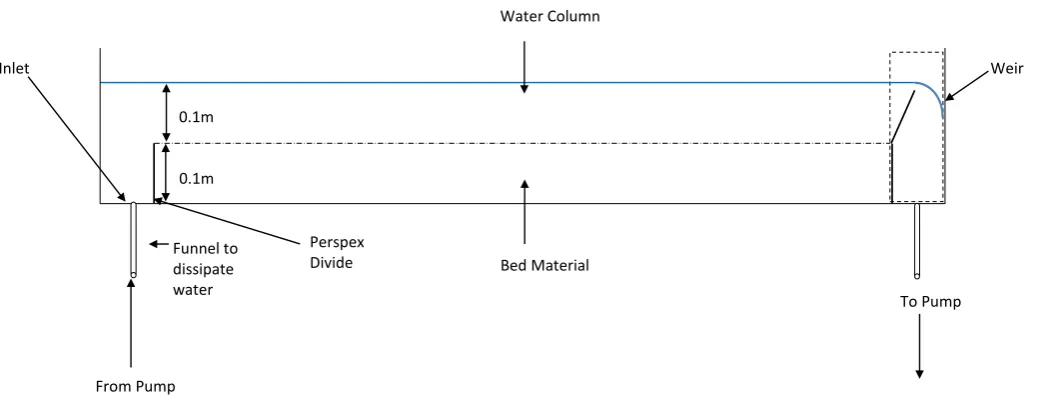
Figure 2.1a: 2D Illustration of the Recirculating Flume Channel...33
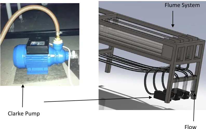
Figure 2.1b: Illustration of flume system design...34
Figure 2.2: Initial Experimental Set Up with Clarke Pump...36
Figure 2.3: Uniformly laid 100 mm gravel bed in situ ...37
Figure 2.4: River Dene catchment showing distribution of Wastewater Treatment Plants along the watercourse...39
Figure 2.5: Establishment of uniform flow...40
Figure 2.6: Turner Designs Cyclops 7 Fluorometer location...42
Figure 2.7: Example calibration profile for Turner Designs Cyclops Fluorometers (in situ calibration: 09.12.2011)...43
Figure 2.8: Wheatstone bridge used with temperature sensor...44
Figure 2.9: Grundfos pump Set Up...46
Figure 2.11: Testing progressive removal of Cyclops Heads from one channel to another to assess impact on oscillation presence...52 Figure 2.12: Experimental set up for light feedback test using black plastic caps
to enclose the LED of the instrument in Rhodamine solution from the surrounding water column to identify if the oscillations are present due to ‘ground loop’ or feedback...53 Figure 2.13: Flume System...55 Figure 2.14: Example trace to illustrate recorded exchange in experimental rig
(Q = 12 l/min; Bed = Glass Bead; Bed-Form = Flat; Flow Depth = 0.03 m; Expected end concentration = 112 ppb; Recorded end concentration = 111.8 ppb; Date = 11/11/2012)...56 Figure 2.15: Analytical procedure used to establish Hyporheic Exchange gradient ...59 Figure 2.16: Obtained values of Marion et al. (2002) overlaid onto O’Connor
and Harvey’s values...60 Figure 2.17: Application of smoothing to trace data extracted from 5 mm sediment trace test...62 Figure 2.18: Decomposition of trace data for analysis providing an example of data analysis utilising GenStat...63 Figure 2.19: Dye trace conducting in 3 different recirculating flume
Figure 2.21b: Trace test outputs after temperature compensation in glass bead test (flatbed; 5 mm sediment) showing difference of concentration and final asymptotic concentration in log scale for 30 hours testing………...67 Figure 2.22: Trace test conducted on flat and undulating gravel beds at a discharge of 12 l/min...68 Figure 2.23: Reverse Sorption test trace; conducted at 12 l/min...69 Figure 2.24a: Repeat discrete injection trace conducted on flat glass bead
Bed...69 Figure 2.24b: Repeat discrete injection traces conducted on flat glass bead bed manipulated for gradient comparison...70 Figure 2.25: Temperature Compensated Raised Glass Bed Trace - 4cm Flow
Depth...71 Figure 2.26: Visual comparison of consecutive doses added to raised fixed glass bed flume test...72 Figure 2.27: Removal of Cyclops fluorometers from water column of flume 8 to
independent flume channels to assess impact on oscillation...72 Figure 2.28: Diagram illustrating the creation of constructive interference from waves...75 Figure 3.1: Hyporheic exchange is the interchange of surface-water with
Figure 3.3: Illustration of the greater potential depth of flow through an undulating bed-form with a smaller wavelength due to increased
connectivity between the dunes...84
Figure 3.4: Clogging effects of microbial communities depending on the effective porosity of hyporheic sediments; taken from Nogaro et al., 2010...86
Figure 3.5: Illustration of differences between potential biofilm developments on different sediment particle sizes...88
Figure 3.6a: Example flat bed profile employed in flume systems to quantify impact of particle size on rate of hyporheic exchange...91
Figure 3.6b: Photograph of sediment in the flume systems...91
Figure 3.7a: The undulating bed-form employed in trace testing...95
Figure 3.7b: The flat bed-form employed in trace testing...95
Figure 3.8: Experimental set up of homogenous sediment experiment to assess impact of sediment particle size on biofilm development...96
Figure 3.9: Placement of extractable glass slides on the sediment surface...101
Figure 3.10a: Schematic of sediment coring to quantify effective depth penetration of microbial development from the bed material at Time End... 102
Figure 3.10b: Example of a sediment coring of bed material at Time End...102
Figure 3.12: Example comparative normalised rate of exchange in experimental systems after initial dye injection at Time 0...108 Figure 3.13: Example comparative rate of exchange in the experimental
systems following Rhodamine tracer injection on 5mm
sediment...109 Figure 3.14: Comparative rate of exchange in the experimental systems...110 Figure 3.15a: Time 0 and Time End visual comparison of biofilm development on different sized glass beads...112 Figure 3.15b: Side View of Time End visual comparison of biofilm development on different sized glass beads...112 Figure 3.16a: Biofilm development on the surface of different bed materials in re-circulating flume system...114 Figure 3.16b: Microbial community depth development on different bed materials in re-circulating flume system...114 Figure 3.17: Flat Bed microbial community development on sediment surface
in flumes of different sediment particle sizes. Error bars represent ± standard error of the mean...115 Figure 3.18: Microbial community depth penetration quantified from TimeEnd
cores. Error bars represent ± standard error of the mean...115 Figure 3.19: Example of temporal variance in normalised hyporheic exchange
rates following bi-daily repeat discrete tracer injection...117 Figure 3.20: Temporal variance in normalised hyporheic exchange gradients
from flat bed flume tests; taken at 30 % exchange...118 Figure 3.21: Example microbial community depth development on 5 mm glass
Figure 3.22: Example of microbial community depth development on 0.5 mm glass beads in undulating (2-dune) flume system...120 Figure 3.23: Example microbial community depth development on 5 mm glass
beads in undulating (multiple) flume system...121 Figure 3.24: Example microbial community depth development on 0.5 mm
glass beads in undulating (multiple) flume system...122 Figure 3.25a: Biomass levels at depth in dune tests. Error bars represent ± standard error of the mean...123 Figure 3.25b: Biomass levels at depth in dune tests. Error bars represent ± standard error of the mean...124 Figure 3.26a: Microbial development at surface in multiple dune tests. Error bars represent ± standard error of the mean...126 Figure 3.26b: Microbial development at surface in two dune tests. Error bars represent ± standard error of the mean...126 Figure 3.27: Variance in Normalised hyporheic exchange gradients from 2 undulating dune flume tests; 30 % exchange...127 Figure 3.28: Variance in normalised hyporheic exchange gradients from multiple dunes flume tests; 30 % exchange...128 Figure 3.29: Temporal variance in normalised hyporheic exchange gradients from multiple dunes flume tests; omitting last sample...138 Figure 4a: Pathways for PNP degradation in bacteria………146 Figure 4.1: Study site for sediment and water collection along the River Dene, Wellesbourne, UK. ...148 Figure 4.2: Experimental units on rotary shaker, incubated in dark conditions
Figure 4.3: Experimental units on rotary shaker in controlled environment room, incubated in light and dark conditions with PNP...153 Figure 4.4: River Dene catchment showing distribution of Wastewater
Treatment Plants along the watercourse in conjunction with the sample sites. ...157 Figure 4.5: The mean biodegradation of PNP under employment of different
physiological components. Error bars represent ± standard error of the mean. ...160 Figure 4.6: The biodegradation of PNP under employment of different light
conditions. Error bars represent ± standard error of the
mean. ...162 Figure 4.7: Mean pH variation in experimental units during testing under
Figure 4.11: Chlorophyll-a content of sediment from different sample sites along the River Dene. Error bars represent ± standard error of the mean. ...169 Figure 4.12: Canonical variate analysis plot of PLFA profiles in different river
sediment sample sites following extraction from the river. Circles represent 95 % confidence intervals. ...169 Figure 5.1: Schematic showing integration of findings from current
research...184 Figure 5.2a: A visualisation demonstrating the variation of the rate of hyporheic
Figure 5.6: Mean chlorophyll-a variation in experimental units during testing under employment of different light conditions………194 Figure 5.7: A. The biodegradation of PNP under employment of different
Glossary of Terms
𝐴𝑠 Surface area of sediment Bed
𝐶∗ Normalised concentration Db Biodiffusivity
Dd Dispersion coefficient 𝐷𝑒 Effective diffusion
𝐷𝑚 Molecular diffusion
𝐷′𝑚 Sediment molecular diffusion M’ Effective Penetration Depth
𝑡 Time
𝑉𝑤 Water volume in flume experiment
𝛽 Sediment diffusion correction term
Acknowledgements
The most rewarding part of this thesis is the ability to reminisce and look back
over the course of my studies and acknowledge the support, guidance, comical
genius and culinary delicacies that have been imparted upon me throughout my
academic endeavours. As such, this acknowledgment section provides initial
opportunity to thank those who have been most influential in encouraging me
through my research.
First and foremost, I would like to thank my supervisors for offering me support
and guidance over the course of the project. Your encouragement, advice,
constructive criticism and occasional creative disparity helped guide me through
my studies. Special thanks should be given to my primary supervisors,
Professor Gary Bending and Dr Jonathan Pearson, without whom this project,
along with my motivation to persevere, would not have succeeded. Their
reassurance, patience and humour sustained my desire to succeed, focused my
energy and encouraged me to proceed; irrespective of the size of the obstacles
placed before me.
I would like to show my gratitude to Unilever and the Natural Environment
Research Council for their financial support, which enabled me to undertake
novel scientific research, liaise with countless collaborators and perform
advanced analysis on my experimental samples. With this said, a special acknowledgement should go to Dr Oliver Price for ensuring Unilever’s goals
were pursued throughout this investigation. This opportunity will also be taken
to say thank you to the members of my Advisory Panel and project
collaborators, particularly Dr Hendrik Schäfer and Professor Alison Rodger, who
I am now, and always will be indebted to numerous people who have helped
me during this project. With that said, special recognition should be made to a
few:
An overwhelming thank you must be given to Dr Julie Jones, the ‘Statistical Guru’ that helped guide me through the turmoil that ensued
from my generation of one of the most colossal data sets she had ever
seen. For introducing me to the weirdly wonderful world of GenStat and
teaching me how to use it, I will be forever in her debt.
The most entertaining and painful thank you must be given Ian Bayliss, a man who can only be described as the ‘Rockstar’ of the engineering
technician world. If it were not for his atrocious jokes, rapid response to
flume floods with the aid of his handy water vacuum and his ability to fix
everything with gaffer tape, silicone or a wrench, my time in the flume
room would have ruined me. So thank you Ian for teaching me how to use
a silicone gun like a professional and for showing me that duct tape and a
hammer can solve every problem.
To the fine individuals that have guided me to the completion of my thesis, I will
always be beholden for your help.
In addition to all of these statements of gratitude, my most heartfelt thankfulness
and appreciations must go out to my family, friends and loved ones. Their
unwavering support and affections throughout provided me with the courage
and the strength to endure when times were tough. Their kind and reassuring
words helped to keep me calm when my experiments misbehaved, making
these wonderful individuals directly responsible for preventing numerous late night ‘modifications’ to my experimental systems.
Moreover, I will always be grateful for the ease at which I could convince
everyone I love to drop what they were doing to come and spend countless
discernible reward for them to speak of, all out of their love of me. To these
people, my arms, back, legs and hands thank you!
Finally, I will never forget the friends that made my experience at Warwick as
memorable as it was. Thank you for ensuring that a more than adequate
amount of my time was spent enjoying university life, playing sports, eating
indescribable food, consuming copious amounts of caffeine and alcohol,
wearing countless fancy dress costumes and, most recently, for helping me
realise that I am a ‘special fluids’ expert. Were it not for you, this thesis would
Declaration
I declare that the work presented in this thesis was conducted by me under the direct
supervision of Professor Gary Bending and co-supervision of Doctor Jonathon Pearson,
Doctor Hendrik Schäfer and Doctor Oliver Price, with the exception of those instances
where the contribution of others has been specifically acknowledged. None of the work
presented has been previously submitted for any other degree.
Abstract
Riverine environments are stressed and damaged by anthropogenic actions, with
chemical contamination a key factor, identified as potentially adversely impacting
the aquatic network. Standardised Organisation for Economic Co-Operation and
Development (OECD) tests are used to establish biodegradation rates of chemicals
in the environment, however these tests are conducted in unrealistic conditions
deficient of environmental realism. Increasing the environmental realism of OECD
tests has the capacity improve prediction of chemical persistence and identify
potential for damage to the environment. Moreover, the interactions between
bed-form, microbial biofilm communities and chemical biodegradation at the
sediment-water interface are not considered in OECD tests. The current project explored the
effects of bed-form characteristics on biofilm development and the consequences
of sediment on biodegradation at the sediment-water interface. Novel flume
systems were designed, constructed and used to develop methodologies to
investigate the impact of bed form on hyporheic exchange. River water and
sediment were sampled from a stretch of the River Dene (Wellesbourne, UK) and
used as microbial inocula in chemical biodegradation studies using a series of
specially designed re-circulating flume systems and ex-situ bottle experiments.
Flume experimentation quantified the rate of microbial community development,
topographical location and effective depth penetration on sediment beds within
artificial watercourses, whilst simultaneously identifying the impact that this biofilm
development possessed on hyporheic exchange. The effects of light and inoculum
source on para-nitrophenol (PNP) biodegradation were also determined following
OECD regulatory test protocols in an attempt to evaluate the realism of chemical
biodegradation tests.
Experimental data showed that microbial development varied on different sediment
bed profiles, and that biofilms significantly reduced the rate of hyporheic exchange
on small (0.5 mm), but not large (2.0 mm) sediment particle size bed materials.
Additionally, this study found that light inhibited PNP degradation in all tests and
that sediment sieving utilised in OECD tests decreased rates of biodegradation of
PNP. This project revealed the importance of microbial biofilms in determining
investigate hyporheic exchange in heterogeneous sediments, whilst developing
Chapter 1
1.1 Introduction
Anthropogenic activity can have detrimental effects upon the environment due to the intertwined nature of ecosystems (Carlow and Petts, 1992; Vitousek et al., 1997). Humanity’s expansion has degraded lotic ecosystems, with increased levels of industrialisation, urbanisation and land use change altering aquatic environments through elevated levels of organic and inorganic waste (Vörösmarty et al., 2010); a situation that is graver in numerous regions of the developing world due to lack of suitable wastewater treatment (Finnegan et al., 2009). One of the main groups of chemicals that are impacting the aquatic environment are daily use consumer chemicals that are disposed of with household waste water (Whelan et al., 2011). Such chemical pollutant influx into aquatic systems can detrimentally impacts the habitability of the environment, causing shifts in biodiversity, structure and functionality of ecosystems (Lake, 2000; Dyer et al., 2003).
Presently, standardised Organisation for Economic Co-Operation and Development (OECD) tests are used as regulatory tests to establish degradability of chemicals and compounds in the environment (Guhl and Steber, 2006). These tests are conducted in unrealistic conditions deficient of environmental realism, often in absence of light and using high concentrations of the test chemical (Ericson, 2007). Increasing the environmental realism of OECD tests will improve prediction of chemical persistence and help to inform potential risk to the environment (Thomas and Hand, 2011).
including the solubility of the chemical and mixing characteristics (Dutton, 2004). The mixing characteristics may be governed by flow rate, sediment characteristics and channel morphology, particularly bed-form (Marion et al., 2002; Bottacin-Busolin et al., 2009). Currently, interactions between bed-form, microbial biofilm communities and chemical biodegradation at the sediment-water interface are not considered in OECD tests (Ericson, 2007). This study focuses on the effect of fluvial bed-form characteristics and microbial biofilm composition on the fate of chemical pollutant distribution and biodegradation and how they compare with OECD testing. This study assesses factors within river systems that influence soluble pollutant biodegradation, focusing on hyporheic exchange and mixing characteristics within the channel.
Hyporheic exchange occurs when the overlying water column transfers solutes into the interstitial solution surrounding porous sediments due to a concentration gradient (Cardenas et al., 2004). Hyporheic exchange affects numerous environmental features, such as the flux of water exchange and provision of attenuation zones for specific pollutants by biodegradation, mixing and sorption (Packman and Brooks, 2001; Environment Agency, 2009). Consideration of hyporheic exchange is crucial when estimating contaminant fluxes in lotic systems; particularly as the bed material and bed form have the potential to control pollutant distribution patterns (Rutherford, 1994; Wondzell, 2006).
Models have been created to assess risk and predict exposure distance and duration in the event of chemical spills in river systems (Technical Guidance Document, 2003 and the Impact Zone Model; see Paul et al., 2005). These models are based on protocols that do not account for real world environmental variables such as biofilms and river morphology, and predominately focus on single variables.
This study investigated the potential importance of multiple variables which could affect pollutant fate in riverine systems, focusing on fluvial bed-form characteristics and microbial biofilm composition (Marion et al., 2002; Bottacin-Busolin et al., 2009).
1.2 “Down-The-Drain” chemicals
The chemical components used by the domestic consumer, such as surfactants, solvents, dyes, perfumes, pharmaceuticals and Triclosan (antibacterial chemical used in toothpaste and soaps), are commonly referred to as Down-The-Drain (DTD) chemicals because they are largely discharged into the sewer water system after use (Keller, 2005). Recently, there has been an increase in the awareness regarding DTD chemicals attributable to heightened concern of potential adverse human and ecological effects resulting from the employment and disposal of chemical products (Lapertot and Pulgarin, 2006). The heightened awareness around DTD chemicals is attributable to the fact that they are often disposed of with household wastewater, with no measurement or regulation of chemical quantities (Whelan et al., 2011). The biggest proportion of DTD chemicals used is within home and personal care products (HPC), such as those found in skin care products, soaps, deodorants, hair care products, household products and laundry products; quantities of which number in the thousands (Richardson et al., 2005).
Recent studies have identified a geographical variance between regional HPC use, showing countrywide disparities. This is seen in the highest estimated use of HPC products in two regions in Europe, Southern England and a transboundary area in Europe containing Belgium, the Netherlands, and Germany (Price et al., 2010) and variance across China, with higher usage in East and South China when compared to the Northwest (Hodges et al., 2011).
The International Association for Soaps, Detergents and Maintenance Products identified that the European total household value of HPCs was estimated at 27.7 billion Euros, showing annual growth of approximately 1%. The majority of HPCs that enter the environment are laundry products, accounting for 48% of this value (url:http://www.aise.eu/).
1.2.1 Pathways of Down the Drain Chemicals into the environment
The amount of DTD chemicals reaching the lotic environment after release is predominately a function of the chemicals’ partitioning behaviour and biodegradation rate. With this said, different levels of development and financial affluence affect the way in which chemicals enter the environment, meaning that there is a large geographical difference seen in water treatment. In developed countries, such as America and parts of Europe, wastewater is treated through wastewater treatment systems (Sperling et al., 2002; Reemtsma et al., 2008). Within typical Waste Water Treatment Plants (WWTP) processes, a measure of the solids is removed during primary treatment (40-60%), with the resulting effluent treated to remove any remaining solids prior to its subsequent release to surface water. Conversely, in the developing world, with a lack of treatment processes, DTD chemicals are released directly, straight from the household into the water system.
chemical substances by microorganisms to CO2 and readily utilisable
biomolecules, and results in the production of new biomass and organic microbial biosynthesis. These HPCs are used on the human body, meaning that prior to entry to the water system they are not subject to metabolic alteration. This means that these chemicals have the potential to enter wastewater, and eventually aquatic environments, unaltered after disposal from households.
With reference to pharmaceutical use, intact and metabolized active chemicals are discharged to the aquatic environment following excretion from the body (Richardson et al., 2005). The major source of human pharmaceuticals in aquatic systems originates from domestic and hospital sewage disposal, which is attributable to use of drugs for treatment of human diseases. In some cases, effluents from aquaculture systems often increase the levels of chemicals reaching the aquatic system due to the use of veterinary drugs (Boonstra et al., 2011).
1.3 Consequences of chemical release into the environment
Chemical environmental fate pertaining to Pharmaceutical Personal Care Product (PPCP) chemicals is starting to become more widely appreciated and understood, however it remains to be adequately documented. However, some persistence data and bioaccumulation values in aquatic organisms have started to be reported in more depth. The widespread employment of antibiotics, for example, is a major cause of the spread of resistance among bacterial pathogens. Exposure to antibiotics can alter the structure of microbial communities and thereby affect the higher food chain (Daughton and Ternes, 1999). Government and industrial sponsors have designed legislation to manage and control the generation, distribution and vending of domestic and personal care products that use persistent, bioaccumulative or toxic chemicals, all of which has resulted in heightened levels of monitoring and chemical investigation.
1.4 Regulatory drivers for chemical management
Chemical regulation is required to monitor the influx and abundance of substances in the environment, in addition to reviewing their application, quantities and concentrations measured in the environment. Anthropogenic activities, particularly those linked to development, have resulted in higher levels of chemical employment, thereby calling for a greater level of understanding of the chemical dissipation processes occurring in the environment.
1.4.1. REACH and PBT assessment
To achieve enhanced and more robust assessments whilst reducing animal testing, information has to be used in an integrated manner. REACH Implementation Projects updated and extended technical guidance documents for risk assessment of new and existing chemicals. This legislation has resulted in new levels of innovation, resulting in the design of safer chemicals and processes that have enhanced corporate responsibility and promoted competition within the European Chemical Industry (Rudén and Hansson, 2010).
Knowledge of the biodegradability of chemicals is an essential requirement for hazard, environmental risk and persistence assessment (ECETOC, 2007), resulting in the production and evolution of international and national frameworks to identify PBT substances and control their emission into the environment. Understanding the mechanisms responsible for chemical persistence (intrinsic, environmental and physical persistence) is therefore important for assessment.
Subsequently, REACH set minimum data requirements to obtain high levels of protection for human health and the environment, which call for adequate standardized information to draw overall conclusions with respect to the regulatory endpoints classification and labeling, for persistent, bioaccumulative and toxic (PBT) assessment and predicted no-effect concentrations (PNEC) derivation (Ahlers et al., 2008).
1.5 Determination of Biodegradation Rates
use and disposal patterns, identification of the physico-chemical properties and the characteristics of the receiving environment.
1.5.1 Predictive Modelling
Prediction of chemical biodegradability in the natural environment is one of the main focuses of researchers as the ability to predict the chemical persistence in the environment lessens the necessity for experimental testing. Several computer models have been generated to predict biodegradability based on a series of calculations that identify the probabilities of individual chemical transformations. CATABOL, for instance, calculates the environmental persistence of chemicals while also generating information on metabolic pathways and identification of stable metabolites (Jaworska et al., 2002). Whereas BIOWIN models estimate the probability of rapid aerobic biodegradation, a model that has been partially validated in subsequent research (Boethling et al., 2003; Posthumus et al., 2005).
1.5.2. OECD tests
1.5.3 Overview of Current Testing
1.5.3.1 Ready Biodegradability Tests
Ready biodegradability tests are first tier tests, identified as providing only limited opportunities for biodegradation and acclimation of the inoculum (Reuschenbach et al., 2003). These tests are conducted in aerobic conditions using high concentration levels of the test substance (OECD Guidelines for testing of chemicals, 1992). The test pass levels have to be reached within 10-days of the 28-day test period. These types of test permit identification of a test compound’s degradability under natural conditions, with a pass indicating the test chemical is degradable. However, this type of test has been suggested to underestimate the potential of degradation in actual environmental systems (Lapertot and Pulgarin, 2006; OECD Guidelines, 2005).
1.5.3.2. Inherent biodegradation tests
1.5.3.3 Simulation tests
Simulation tests are conducted in aerobic and anaerobic conditions, designed to provide data for chemical biodegradation rates under specified environmentally relevant conditions. These are provisionally designed to replicate and assess the rate and extent of biodegradation in either the aerobic treatment stage of a WWTP or environmental compartments. The tests add an additional layer of testing, incorporating indigenous biomass, media, or relevant solids (e.g. soil, sediment) to assess sorption of the test chemical and replicate a particular set of environmental conditions. These tests are designed to employ biodegradation kinetics that mimic the actual environmental conditions more closely, employing lower concentrations of the test chemical (e.g. less than 1 μg/L to 100 μg/L).
Chemical fate in WWTPs is often investigated in the laboratory setting via employment of simulation tests, particularly those that assess the impact of Activated Sludge Units (OECD 303 A) and Biofilms (OECD 303 B) on experimental chemicals. Monitoring changes in Dissolved Organic Carbon (DOC) and/or Chemical Oxygen Demand (COD) identifies the biodegradation of the test chemical (Comber and Holt, 2010).
1.6. Environmental realism of tests
It is possible to conduct higher tier biodegradation tests to identify the biodegradation kinetics of test substances; the duration of these tests together with their cost and complexity reduces their suitability as standardised protocols (Merrettig-Bruns and Jelen, 2009). Resultantly, OECD tests are conducted to assess the biodegradation rates of test chemicals, however they do not take into account the variations seen in natural environments, particularly the water chemistry, inoculum concentration and composition, environmental context, the test substance concentration or the global relevance.
1.6.1. Effect of environmental factors on biodegradability assessment
sp. isolate within 120 hours if not impacted by pH (optimum pH 8-9). It has also been discovered that longer degradation times occur at lower temperatures (Kang and Kondo, 2002).
The rationale behind generating a standardised test protocol for chemical degradation studies that omit variability in environmental parameters is to simplify the test system so that it is not impeded by variables that will not be replicated in all environmental systems, thereby standardising its application possibilities. For example, light is not present in biodegradation tests to avoid algal development and prevent it from affecting the biodegradation of tested chemicals or alter the possible interpretation of CO2 data analysed in such tests
due to fixation. There are an abundance of environmental parameters that vary from watercourse to watercourse, making standardisation of testing necessary. However, in order to standardise testing to permit ‘accurate’ modelling of chemical biodegradation, a plethora of environmental parameters are not taken into consideration. These parameters include temperature, which affects bacterial growth and biomass (White et al., 1991), pH which may alter the toxicity of environmental pollutants (Rutgers et al., 1998; Li et al., 2008), chemical mineralization (Boyd et al., 1983), channel morphology and channel flow dynamics that impact contact of chemicals with bacteria on the sediment surface (Kunkel and Radke, 2008) and the biofilm community structure and function (Battin et al., 2003).
1.6.2. Water chemistry
Across the length of an impacted river the biota ‘self-purifies’ the environmental compartment, degrading chemicals that enter the water column. This biotic recovery is the river’s natural resilience to environmental disturbance, often dependent on increases in Dissolved Oxygen (DO) and nitrification. The further
potential effects of DTD chemicals that enter watercourses (McAvoy et al., 2003).
[image:42.595.122.554.164.367.2]1.6.3. Inoculum
Ex-situ laboratory studies employed to assess chemical biodegradation rates in the environment are most realistic when conducted using mixed culture systems extracted from the field (Spain and Veld, 1983). However, numerous experimental factors must be controlled when running biodegradation studies as the biodegradation rate can be impacted by variance in experimental factors, such as temperature, pH, salinity and microbial biomass (Spain and Veld, 1983; Thouand et al., 1995). If laboratory studies are to be used to predict biodegradation rates in the field, it is important that the rate-determining factors are understood (Spain and Veld, 1983) and controlled (Thouand et al., 1995).
Additionally, previous work has shown that adaptation of microorganisms can also play a major role in determining biodegradation rates (Feslet et al., 1981). Adaptation is defined here as a change in the microbial community that increases the rate of transformation of a test compound as a result of a prior exposure to the test compound. All of these variables result in differences in inocula used in simulation tests. As biodegradability tests may involve inoculum from different origins, inocula source should also be taken into account while running tests (Thouand et al., 2011) as surface water, sediment and soil samples all support different community structures of microbial composition, diversity and abundance. The influence of this inoculum variability on biodegradation tests is attributable to the source and concentration of live bacteria, the adaptation of bacteria to the test molecule and the presence of protozoans from the natural environment (Barkay and Pritchard, 1988; Thouand et al., 1995). It is therefore imperative to control the number of specific biodegraders used in biodegradation tests to limit the risk of errors in biodegradability tests (Thouand et al., 1995; Forney et al.,2001).
1.6.3.1. Biofilm as inoculum
The microbiology of rivers and streams, and its subsequent impact on biodegradation, has been very much neglected (Neu and Lawrence, 2006). This is most likely attributable to the difficulty associated with in-situ study and/or the use of laboratory models of lotic systems (Left, 1994). Irrespective of this, the interfaces in these constantly changing ecosystems contribute significantly to the geographical distribution and constant recycling of contaminants and nutrients in all flowing water systems (Lock, 1993; Neu and Lawrence, 2006).
surfaces (Vinten et al., 2011). Research conducted on the presence of biofilm communities within lotic systems has identified these communities as an influencing factor in the removal of contaminants from the water column, thereby enhancing the self-purification of surface waters (Edwards et al., 1990).
The development of biofilm communities on the sediment bed results in them acting as the first boundary that interacts with dissolved substances entering and being transported along the water column. Biofilms possess the capacity to integrate the effects of environmental conditions over extended periods of time due to their rapid growth rates and the physiological variety of the organisms from which they are formed. As such, standardized methods of biofilm extraction from river ecosystems could be applied to biodegradation testing where biofilm is employed as inoculum, as numerous studies have identified biofilms as possessing a significant impact on the rate of chemical biodegradation (Araya et al., 2003; Tien et al., 2011). Moreover, as chemical biodegradation is often species specific, requiring a certain species of bacteria to degrade a specific chemical, biofilms possess the capacity to act as natural microbial populations in testing due to their reflection of the actual river environment (Thouand et al., 2011). Furthermore, modifications in bacterial communities may be attributable to the disruption of important ecosystem processes which have the capacity to impact chemical presence in water/sediment systems. As such, detection of microbial community modifications is important for monitoring the effects of chemicals in river ecosystems, and in turn, enhancing chemical risk assessment.
1.7 Hyporheic Exchange
diverse zones within lotic systems, where active mixing occurs that follows chemical gradients due to the mixing of groundwater and surface water by fluvial fluxes, all of which supports an ecotone of benthic macroinvertebrates and fish (Gibert et al., 1994; Williams and Hynes, 1974). The speed and extent of hyporheic exchange is governed by flow interactions with the channel morphology and the resultant rate of hyporheic exchange (Harvey and Bencala, 1993; Elliott and Brooks, 1997).
Stream-subsurface exchange processes are important because of their role in controlling the transport of contaminants and ecologically relevant substances in streams (Packman et al., 2004). These exchanges have the capacity to affect numerous environmental features, ranging from controlling the flux of water exchange to the provision of attenuation zones for specific pollutants by biodegradation, mixing and sorption (Packman and Brooks, 2001; Environment Agency, 2009).
1.7.1 Solute Transport
Solute transport is one of the most crucial driving forces in riverine systems, influenced by chemical, biological and physical processes, the magnitude of which is dependent upon both the environmental parameters and the solute properties (Ng and Yip, 2001). Following point source pollution events, modelling identifies the point downstream that pollutant will cease to affect the watercourse (Dutton, 2004). This is affected by solute transport mechanisms which impact the rate of hyporheic exchange of soluble particulates from the overlying water column to the interstitial fluid in the sediment bed across a sediment-water interface (O’Connor and Harvey, 2008). There are two processes that operate to mix suspended solutes: advection and diffusion. Advection is the bodily movement of a mass of fluid by flow regime, changing physical or chemical properties of the fluid (Chanson, 2004). Diffusion is the movement of liquid particles as a result of thermal agitation from an area of high concentration to an area of lower concentration (Chanson, 2004); this can be either molecular or turbulent. Advective transport moves the solute away from the source point with bulk fluid movement and thus providing the suspended particulates similar velocities to the fluids in the channel (Ng and Yip, 2001). Diffusion spreads the solute transversely and longitudinally throughout the channel along a concentration gradient resulting from turbulence, molecular and/or effective diffusion (Chanson, 2004).
1.7.2 Diffusion
1.7.2.1 Molecular Diffusion
Molecular diffusion occurs in stationary fluids when high concentrations of solute are added to the overlying water column, creating a concentration gradient causing the solute to spread in all dimensions due to random molecular movement, eventually extending across the sediment-water interface and spreading through the pore water (Rutherford, 1994). Rutherford (1994) states that Fick’s first law explains this diffusion as the rate of particle movement is comparative to the spatial concentration gradient (O’Connor and Harvey, 2008).
The rate of molecular diffusion through the hyporheic layer is directly affected by sediment, as solute must navigate the sediment particles to gain access to the pore water, reducing the molecular diffusion coefficient. Theoretical and empirical studies show molecular diffusion coefficients (D’m) are calculated by
taking porosity and tortuosity into account (Berner, 1980), thereby generalising the sediment molecular diffusion expression to:
𝐷′𝑚 = 𝛽𝐷𝑚
Where Dm is the rate of molecular diffusion and 𝛽 (sediment diffusion correction
term) signifies the empirical expression for tortuosity as a function of porosity (𝜃) (see Iversen and Jørgensen, 1993, for further description).
1.7.2.2 Effective Diffusion
natural systems are complex and a combination of processes cause net hyporheic exchange. These processes include molecular diffusion, advective pumping, sheardriven flow, turbulent surface penetration and hyporheic water mixing (O’Connor and Harvey, 2008). Presently, no singular theory exists to predict the resulting exchange in terms of bed parameters or measured streams. Instead, bulk solute exchange across the sediment water interface can be modelled with an effective diffusion coefficient that includes all the factors that influence hyporheic exchange. This can be shown formulaically by:
𝐷 = 𝛽(𝐷𝑚+ 𝐷𝑏) + 𝐷𝑑
Where: Db is the biodiffusivity and Dd is the dispersion coefficient,
encompassing turbulent diffusion and pumping (Berg et al., 1998).
According to O’Connor and Harvey (2008), it is possible to obtain a measured value of effective diffusion using a tracer, where hyporheic exchange forces the tracer placed in the channel into the pore spaces of the sediment bed, resulting in fluid exchange from the bed sediment to the water column over time.
O’Connor and Harvey’s (2008) analysis of hyporheic exchange investigations identifies a scalar relationship to predict the rate of mass transfer in near surface sediments which is applicable to all flow and substrate parameters. This data quantifies net hyporheic exchange using an effective diffusion coefficient incorporating all the transport processes, using dimensional analysis to scale effective diffusion to shear stress velocity, roughness height and permeability to describe sediment and flow characteristics (O’Connor and Harvey, 2008). This analysis created the effective diffusion (De) formula for tracer experimentation,
providing a representative analytical calculation for hyporheic exchange:
𝐷𝑒 = (√𝜋2
𝑉𝑤
𝐴𝑠
𝑑𝐶∗
Where Vw is the volume of water, As is the surface area of the sediment bed, C*
is the normalised concentration and t is time.
1.7.3 Pumping
Changes in channel bed-form cause fluctuations in pressure distribution over the bed. Changes in bed topography modify the flow gradient and create pressure variations which cause pumping in porous bed sediments, a process which alters flow through streambed sediment (Packman and Bencala, 2000). Channel flow impediments, such as bed-forms, create high-pressure regions upstream of the obstruction and low pressure downstream. This pressure gradient results in the overlying water being driven into the interstitial porous spaces within the sediment bed store, travelling through the obstruction and then exiting downstream of the obstacle. These processes, known as upwelling and downwelling correspondingly, create hyporheic circulation under the obstruction (Tonina and Buffington, 2007). This process is illustrated in Figure 1.2, showing tracer movement though bed-form, driven by pumping flow. The presence of bed forms such as dunes, therefore, theoretically alters the rate of mixing within the channel, affecting mass transfer into the bed (O’Connor and Harvey, 2008).
Models that predict mass transfer into the sediment (Elliot and Brookes, 1997) by pumping have been devised in order to quantify hyporheic exchange by examining the sediment domain. O’Connor and Harvey (2008) built on this and created a formula to calculate the effective depth of solute penetration as a result of pumping, using the same parameters used to derive effective diffusion which considers amplitude, wavelength and particle size.
𝐷𝑒 = (√𝜋2
𝑑(𝑀′/𝜃) 𝑑(𝑡1 2⁄ ))
2
Figure 1.2: Schematic example of potential pumping movement through a bed-form compared against an enhanced experimental tracer photograph of a similar bed-form, illustrating the tracer movement through the bed via pumping (image taken from Dutton, 2004).
Direction of Flow
Dye Injection
Injection site of tracer
Tracer movement through bed-form Potential flow path water through sediment
1.7.4 Previous Experimental Testing analysing exchange
The following sections identify previous experimental study into hyporheic exchange, both in the laboratory and in the field. The majority of the laboratory studies detailed were incorporated into O’Connor and Harvey’s [2008] effective diffusion scaling relationship.
1.7.4.1 In-situ Testing
There are a limited number of in-situ field experiments that have tried to assess hyporheic exchange when compared to laboratory investigations. The favoring of ex-situ testing is due to the complexity surrounding the environmental system, particularly in terms of quantifying all of the parameters that influence the exchange and generating a method to accurately measure exchange with all the other variables present. The majority of previous investigations used transient storage models to determine the hydraulic parameters and mixing coefficients, including hyporheic exchange.
1.7.4.2 Ex-situ Testing
Due to the environmental variability of in-situ testing, ex-situ experimentation has been favoured due the investigators’ ability to more closely control and monitor the experimental parameters. This can be seen in the employment of flume systems in the vast majority of modern experimental work, in which all parameters are maintained to permit the isolation and investigation of one variable.
This can be seen in the work of Dutton (2004), who maintained all experimental parameters as constant during testing apart from the bed-form; permitting analysis of bed-form in large scale flume tests. Conversely, the work of Chandler (2012) assessed the impact of sediment size and velocity on exchange; employing a novel system that permitted alteration of a single variable at a time, thereby removing experimental variance that would otherwise be found in natural systems.
1.7.5 Predicting Scaling Relationships
A plethora of methods have been proposed for accurate modelling of hyporheic exchange (see Packman and Bencala, 2000). However, these methods do not take flow variations or alterations in sediment characteristics into account, resulting in disparities between models and recorded data. Resultantly, O’Connor and Harvey (2008) collated data from hyporheic exchange flume experiments to create a data set encompassing a large spread of flow and sediment conditions. A measured effective diffusion coefficient was calculated for each study, however the varying experimental systems required different calculations to be employed based on injection and sampling locations (i.e. bed or channel).
coefficient, which demonstrates a strong correlation between the Péclet permeability number and shear Reynolds number.
1.8 Biofilms
The formation of biofilms is a complex multi-functional process in which microorganisms grow on a surface and produce extracellular polymers, resulting in alterations in the organism phenotype (Singh et al., 2006). In rivers, biofilms are predominately attached to sediments. The formation of a functional biofilm (Figure 1.3) starts with irreversible attachment and establishment, followed by maturation and finally detachment (Madigan and Martinko, 2006). Biofilm formation and development is regulated by environmental factors like pH, nutrient and oxygen availability; which all cause biofilm variance (Fux, 2005).
Biofilms enhance microorganisms’ chances of survival and development as embedment within the adhesive EPS matrix results in an altered phenotype with growth rate and gene transcription (Denyer et al., 1993). Organisms within biofilms communicate and coordinate their actions using signalling molecules known as quorum sensors (Kjelleberg and Molin, 2002). This structural communication enables dispersal of nutrients when there is heightened competition for food at high cell densities within the biofilm (Stanley and Lazazzera, 2004). Amalgamation of bacteria into microbial communities enables them to withstand increases in shear forces, pH changes, nutrient deprivation and chemical fluxes due to mechanical strength and support provided by the EPS (Davey and O’Toole, 2000), whilst also transferring exopolysaccharides to higher trophic levels (Decho, 1990; Denyer et al., 1993).
The dense, packed structure of biofilms result in autocatalytic promotion of gene transfer, enhancing the physiological and catabolic performance of complex communities by the formation of new degradation pathways (Denyer et al., 1993; Fux, 2005; Singh et al., 2006). This transfer of plasmids may encode beneficial traits, such as the ability to degrade pollutants, thereby making biofilms useful as a form of bioremediation (Decho, 2000; Fux, 2005).
1.9 Study Objectives
Studies of lotic systems are regularly identifying rivers as biogeochemical hotspots that possess the capacity to process influxes of organic matter that enters the aquatic environment (Battin et al., 2009; Mulholland et al., 2008). Research has suggested that most biological and chemical interactions occur within the hyporheic zone, with suspended solutes interacting at the water-sediment interface. The water-sediments at this interface act as host for microbial biofilm colonisation, which have the potential to influence biogeochemical transformations within the river (Battin et al., 2008). This finding has identified the need to research the variables controlling microbial community development.
Provisional flume testing and other research, such as that of Nogaro et al. (2010), has indicated that microbial community abundance and distribution differs on sediments with different sized particles. The variance in microbial community development fluctuates drastically when in-situ heterogeneous sediments are examined, making it difficult to quantify the impact of biofilm development on exchange (Nogaro et al., 2010). Moreover, mixing characteristics are governed by flow rate, sediment characteristics and channel morphology. Currently, interactions between bed-form, microbial biofilm communities and chemical biodegradation at the sediment-water interface have not been studied in depth. To reach a stage where enhanced modelling can be conducted, experimentation and data collection must take place. This investigation aims to explore the effect of bed-form characteristics on the diversity and pollutant-degrading potential of microbial biofilm communities at the sediment-water surface, and the subsequent impact biofilm development and bed-form has on hyporheic exchanges. The aims assessed in this research project are:
2) Assess the impact of bed-form on the rate of hyporheic exchange and identify the impact biofilm presence possesses on the rate of hyporheic exchange (Chapter 3)
Chapter 2
Flume Development
2.1 Introduction
Hyporheic exchange occurs when the overlying water column transfers solutes into the interstitial solution surrounding porous sediments due to a concentration gradient (Cardenas et al., 2004). Such stream-subsurface exchange processes are important because of their role in controlling the transport of contaminants and ecologically relevant substances in streams (Packman et al., 2004). This exchange affects numerous environmental features, from controlling the flux of water exchange to provision of attenuation zones for specific pollutants by biodegradation, mixing and sorption (Packman and Brooks, 2001; Environment Agency, 2009). Such exchange is governed by flow rate, sediment characteristics and channel morphology (Rutherford, 1994). Consideration of hyporheic exchange is crucial when estimating contaminant fluxes in lotic systems; particularly as the bed material and bed form have the potential to control pollutant distribution patterns (Rutherford, 1994; Wondzell, 2006).
Currently, interactions between bed-form, microbial biofilm communities and chemical biodegradation at the sediment-water interface have not been studied in depth. To reach a stage where accurate modelling of exchange processes can be conducted, experimentation and data collection must take place.
role of individual factors affecting exchange processes in river systems (Williams, 1970). Additionally, recent in-situ riverine experimental studies have emphasised the necessity to conduct more in depth experimental studies to explore the consequences of microbial sediment clogging in the hyporheic zone (Nogaro et al., 2010).
Laboratory flume studies permit simulation of natural environments in a controlled manner, using water and sediment in quantities small enough to control (Friedrich et al., 2007; Williams, 1970). Natural riverine environments contain different boundary conditions than those typically found in laboratory flumes, however the unsteady flow conditions, intermittent sediment and water supplies, nutrient fluxes and other uncontrollable variables in different rivers prevents controlled experimentation (Friedrich et al., 2007). Conversely, laboratory based studies permit efficient investigation of water-sediment interaction under controlled conditions, which can then be used to predict fluvial responses to specifically predefined criteria.
The aims of the work presented in this chapter were:
1) Design and build a flume system suitable for investigating hyporheic exchanges
2) Develop methodologies for assessing hyporheic exchange in the flumes