Distributed resource management across process boundaries

warwick.ac.uk/lib-publications

Original citation:

Suresh, Lalith, Bodik, Peter, Menache, Ishai, Canini, Marco and Ciucu, Florin (2017)

Distributed resource management across process boundaries. In: SoCC '17 Symposium on

Cloud Computing, Santa Clara, California, 24-27 Sep 2017. Published in: SoCC '17

Proceedings of the 2017 Symposium on Cloud Computing pp. 611-623.

Permanent WRAP URL:

http://wrap.warwick.ac.uk/92926

Copyright and reuse:

The Warwick Research Archive Portal (WRAP) makes this work by researchers of the

University of Warwick available open access under the following conditions. Copyright ©

and all moral rights to the version of the paper presented here belong to the individual

author(s) and/or other copyright owners. To the extent reasonable and practicable the

material made available in WRAP has been checked for eligibility before being made

available.

Copies of full items can be used for personal research or study, educational, or not-for profit

purposes without prior permission or charge. Provided that the authors, title and full

bibliographic details are credited, a hyperlink and/or URL is given for the original metadata

page and the content is not changed in any way.

Publisher’s statement:

"© ACM, 2017. This is the author's version of the work. It is posted here by permission of

ACM for your personal use. Not for redistribution. The definitive version was published in

SoCC '17 Proceedings of the 2017 Symposium on Cloud Computing pp. 611-623.,

http://dx.doi.org/10.1145/3127479.3132020

A note on versions:

The version presented here may differ from the published version or, version of record, if

you wish to cite this item you are advised to consult the publisher’s version. Please see the

‘permanent WRAP url’ above for details on accessing the published version and note that

access may require a subscription.

Boundaries

Lalith Suresh

VMware Research Group

Peter Bodik

Microsoft Research

Ishai Menache

Microsoft Research

Marco Canini

KAUST

Florin Ciucu

University of Warwick

ABSTRACT

Multi-tenant distributed systems composed of small services, such as Service-oriented Architectures (SOAs) and Micro-services, raise new challenges in attaining high performance and efficient resource utilization. In these systems, a request execution spans tens to thou-sands of processes, and the execution paths and resource demands on different services are generally not known when a request first enters the system. In this paper, we highlight the fundamental challenges of

regulating load and scheduling in SOAs while meetingend-to-end

performance objectives on metrics of concern to both tenants and operators. We design Wisp, a framework for building SOAs that transparently adapts rate limiters and request schedulers system-wide according to operator policies to satisfy end-to-end goals while responding to changing system conditions. In evaluations against pro-duction as well as synthetic workloads, Wisp successfully enforces a range of end-to-end performance objectives, such as reducing av-erage latencies, meeting deadlines, providing fairness and isolation, and avoiding system overload.

CCS CONCEPTS

•Computer systems organization→Cloud Computing;n-tier ar-chitectures;

KEYWORDS

Microservices, Service-Oriented Architectures, Resource Manage-ment, Rate Limiting, Scheduling.

ACM Reference Format:

Lalith Suresh1, Peter Bodik, Ishai Menache, Marco Canini, and Florin Ciucu. 2017. Distributed Resource Management Across Process Boundaries. In Proceedings of SoCC ’17, Santa Clara, CA, USA, September 24–27, 2017, 13pages.

https://doi.org/10.1145/3127479.3132020

1_{Part of the work was done while at Microsoft Research.}

Permission to make digital or hard copies of all or part of this work for personal or classroom use is granted without fee provided that copies are not made or distributed for profit or commercial advantage and that copies bear this notice and the full citation on the first page. Copyrights for components of this work owned by others than the author(s) must be honored. Abstracting with credit is permitted. To copy otherwise, or republish, to post on servers or to redistribute to lists, requires prior specific permission and/or a fee. Request permissions from [email protected].

SoCC ’17, September 24–27, 2017, Santa Clara, CA, USA

© 2017 Copyright held by the owner/author(s). Publication rights licensed to Association for Computing Machinery.

ACM ISBN 978-1-4503-5028-0/17/09. . . $15.00

https://doi.org/10.1145/3127479.3132020

1

INTRODUCTION

Many organizations including Netflix, Amazon, Uber, SoundCloud, Google and Spotify have adopted Service-oriented Architectures (SOAs) [25] and Micro-services [52] to build large-scale Web ap-plications [8,47,48,53,64,70] and infrastructure systems [3,71].

SOAs comprise fine-grained, loosely coupledservicesthat

commu-nicate via lightweight API calls over the network. Every service

comprises multipleservice instancesor processes, each running

inside a physical or virtual machine. For instance, Netflix has sepa-rate services for managing movie and user data, authentication, and recommendations [49]. Typically, these divisions align with

devel-oper team structures [53]. These systems are commonly shared by

multipletenants, where tenants may represent different external cus-tomers or consumers, but also internal product groups, applications, or system background tasks.

SOAs have three characteristics that complicate managing their end-to-end latency and throughput. First, request execution in SOAs spans tens to hundreds of services, forming a DAG across the service

topology [37]. The exact structure of the DAG is often unknown

when the request first enters the system, since it depends on multi-ple factors like the APIs invoked at each encountered service, the supplied arguments, the content of caches, as well as the use of load balancing along the service graph. Second, by design, individual services in SOAs lack end-to-end visibility into the service topology and by extension, the request execution graph; in fact, services view each other as black boxes. Third, requests from different tenants

contend forsharedresources within individual processes of a

ser-vice such as threadpools, locks, blocking queues, and connection objects. Isolation mechanisms at the host OS or hypervisor fail here, as they lack visibility into the existence of multiple tenants as seen by individual processes.

Unfortunately, existing libraries [50,69] for building SOAs are ill-equipped to deliver on the above performance objectives. These libraries require extensive tuning of static thresholds for rate lim-iters, circuit breakers [17], and timeouts to regulate both load and latency. Setting these thresholds manually in a complex distributed system is fragile and becomes out of date quickly as systems evolve and workloads change [39,51]. Furthermore, several case studies highlight how complex interactions in SOAs not only lead to sharp degradation in performance (e.g., lower throughput and higher laten-cies), but also trigger cascading behaviors that result in wide-spread application outages [7,32,34,68]. These challenges necessitate adaptive, end-to-end resource management for SOAs.

In this paper, we highlight the unique challenges involved in meeting the above performance objectives in multi-tenant SOAs, which are fundamentally different than typical network scenarios. Our key contribution is the design of novel adaptive techniques for SOAs that leverage existing building blocks (rate limiters and request

schedulers) to meet end-to-end performance goals,despitethe lack

of global visibility into request execution DAGs and their load at every service. These techniques are embodied in Wisp, a framework for managing resources in SOAs with minimal operator intervention. Wisp’s design hinges on the observation that rate limiting and scheduling mechanisms at each process, only informed by measure-ments of their local neighborhood, suffice to realize a broad set of performance policies in SOAs. Wisp uses rate-limiting and back-pressure mechanisms that operate at the granularity of groups of

requests which we termworkflows. Wisp rate limits workflows such

that they share resources at every process according to throughput-related policies, e.g., bottleneck fairness [45] or dominant resource fairness [26]. Wisp also operates at the level of individual requests and prioritizes their execution at each process according to latency-related policies, such as Earliest Deadline First (EDF) [65] or Least Slack Time First (LSTF) [35].

Enforcing the above policies, however, requires end-to-end knowl-edge of bottlenecks in the service topology, and characteristics of the request execution graphs. Wisp overcomes these obstacles through several mechanisms. Wisp uses causal propagation of workflow identifiers throughout the system to attribute resource utilization to individual workflows. It then uses a novel distributed rate

adapta-tion mechanism §4.1, where upstream services throttle workflows

according to bottlenecks that emerge on their execution graph. The aggressiveness of the throttling is determined through a configurable parameter that tunes a tradeoff between high utilization and the request drop probability (due to overload). Lastly, Wisp realizes end-to-end variants of policies such as EDF and LSTF by dynamically estimating end-to-end properties of each request (e.g., remaining processing time). Importantly, Wisp decouples policy from mecha-nism, and meets different performance objectives by only leveraging building blocks that are already present in typical SOAs (namely, rate limiters and schedulers). Our contributions are:

•We present characteristics of SOAs through a measurement

study of large production systems (§2) and highlight fundamental

challenges in meeting end-to-end performance objectives in multi-tenant SOA settings (§3).

•We design Wisp (§4), a framework to enforce a diverse range

of resource management policies in SOAs by adaptively tuning rate limiters and schedulers based only on local measurements at each

0.00 0.25 0.50 0.75 1.00

0 50 100 150 Unique services

per workflow

ECDF

0.00 0.25 0.50 0.75 1.00

0 20 40 60

Workflows per service

ECDF

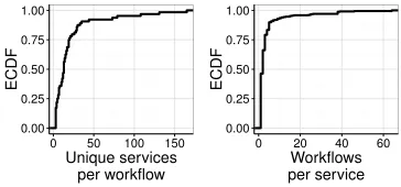
Figure 1: Workflows in production.

process. Importantly, Wisp achieves these goals throughfully

dis-tributedmechanisms, without requiring prior knowledge of request execution graphs and resource demands.

•We evaluate a Wisp prototype (§6). Our results show that Wisp enforces a wide range of performance objectives such as avoid-ing cascadavoid-ing failures, meetavoid-ing soft end-to-end deadlines (e.g., 10x improvement in the 99th percentile latency-deadline ratio), and iso-lating low-latency workflows from high-throughput workflows (2x improvement in average latencies).

2

SOAS IN PRODUCTION

We now discuss relevant characteristics of SOAs using a combination of measurements from a large cloud provider and prior reports on systems from other environments [8,37,47,48,53,64,70].

2.1

Services, processes and workflows

A single application such asbing.com,amazon.com, ornetflix.com

is composed of multiple services. These services are typically main-tained by separate teams (or even third parties) and communicate exclusively over well-specified APIs [52]. Each service runs multi-ple instances (OS processes), distributed across multimulti-ple servers or virtual machines. Requests are dispatched to instances based on the type of service; for example, requests can be load-balanced among processes of a stateless service, whereas routing in stateful services is typically based on some form of hashing. While a request typically enters the system through anentry pointservice such as a set of fron-tend web servers, requests may also originate from internal systems that access shared infrastructure services. A workflow represents application-specific “groups" of requests,that form an execution DAG across a set of services [37]. For instance, all requests from the same tenant may be classified as the same workflow.

2.2

Analysis of shared services

Bing.Figure1presents characteristics of the Bing SOA [37]. Here, each workflow is an execution DAG, and corresponds to dif-ferent features of the larger offered application (including, but not limited to, web, video, and image search). These workflows contend for shared, in-memory resources such as threadpools at different services.

!"!!#$ !"!#!$ !"#!!$ #"!!!$ #!"!!!$

# % #& &%

!

"

#

$

%&

'

(

)'

!

)

*

'

"

+

)&

(

)

,

-"

.

&$

-)

/

'

0

%)

'

!

)

#

11

)

*

'

"

+

)&

(

)

,

2

,

%

-3

4

!"#$%&$'("()*$'"*#+,$''$-".)" /"'$#01,$#Workflows processed by a service

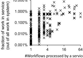
Figure 2: Fraction of overall request processing time spent per service in production. Each dot is a service, x-axis is the number of workflows in that service, y-axis is the fraction of overall processing time spent per-service.

For instance, 24 services are shared by at least 10 different work-flows, with two services supporting 64 unique workflows. These workflows have further semantics that affect their performance needs (e.g., requests from real users require higher priority in the system than those from bots).

Importantly,shared services(services processing two or more

workflows) are responsible for a large fraction of overall request processing time (or work) in the system. Misbehaving workflows in shared services can impact throughput and latency for other work-flows (§2.4). We traced processing time statistics for each workflow

across all services (Figure2). We observe that 53.7% of services

process at least two workflows.Nevertheless, they account for a

much larger fraction of the total work: 86% of request processing time in the system is spent within shared services; 53% within ser-vices that handle 5+ workflows, and 31% within serser-vices handling 10+ workflows. Shared services are therefore critical for end-to-end performance.

Azure Storage.We also consider the Azure Storage platform [13]. It supports tens of external APIs, corresponding to reads, inserts, deletes and scans of both data and metadata. The system comprises services shared across workflows such as the front ends (FE), parti-tion servers (PS), and extent nodes (ENs). The total CPU cycles for serving a request within a service canvary by up to four orders of magnitudeacross workflows [46]. Such variability calls for careful resource accounting and management, e.g., to avoid starvation of short requests. We discuss more characteristics about the system in the evaluation (§6).

2.3

Opaque request execution DAGs

A crucial aspect of request execution in all these SOAs is theopacity

of the execution graph and its corresponding resource consumption at each service. That is, each service is typically oblivious to the

(i)end-to-end execution graph of the request, which depends on

load balancing, multiple levels of caching, number of instances per service, and API parameters used to invoke different services,(ii) request amplification, wherein a single request at an upstream service might correspond to thousands of requests at a downstream service, and(iii) request cost, where different requests at an upstream service may have varying costs further downstream; for instance, the cost of loading an object inAzure Storageis proportional to the object size and is potentially unknown when a request first enters the system at

an entry point. Lastly, request execution characteristics may change as the codebase for individual services evolve, further aggravating the opacity of request execution graphs [39].

2.4

Shared services and outages

The fact that different workflows contend for common resources within shared services has led to outages among production

sys-tems. Visual Studio Online experienced an outage [34] caused by

an interaction of two different workflows in a hierarchy of services. A single workflow was accessing a slow database deep in the ser-vice hierarchy. The blocking RPC calls from the upstream serser-vice eventually exhausted the service’s thread pool. This subsequently

starvedother unrelatedrequests that were trying to connect to an

authentication service, causing widespread application unavailability. A similar interaction across tiers led to an Amazon AWS outage [32]. Services therefore have to be aware of potential bottlenecks among their downstream services. In another episode, a slowdown of some Amazon EBS instances triggered a sequence of bottlenecks in

re-lated services. During the firefighting effort, operatorsmanually

intervenedto throttle upstream EC2 service APIs to reduce load on the downstream EBS service, which affected more customers than

necessary [7]. Such manual intervention is challenging and error

prone.

3

OVERVIEW OF WISP

Wisp is a framework for building SOAs that enables end-to-end resource management for diverse request types. Wisp creates groups calledworkflows, defined as a set of requests that belong to the same class or tenant and are bound by the same resource management cri-teria. Tagging workflows provides fine-grained visibility into request execution, which facilitates attribution of resource utilization and processing activity to specific request groups. It allows processes to differentiate between requests that are causally connected to dif-ferent workflows. Wisp enforces resource sharing policies through

workflow-levelmechanisms. In addition, Wisp usesrequest-level

mechanisms to prioritize request execution according to latency-related policies. For instance, in theBing SOAdiscussed in §2.2, each request type may be classified as a workflow, allocated a fair share of resources, and scheduled according to its urgency. On the other hand, all requests originating from bots can be treated as a low priority workflow, and be scheduled with no deadline targets.

In this section, we describe the performance goals of Wisp (§3.1), and highlight the challenges in achieving them in a distributed setting

(§3.2). We then present in §3.3the main building blocks of our

solution. A detailed description of the design follows in §4.

3.1

Performance objectives

We note that there are two classes of performance objectives of interest in the SOA setting.

The first class pertains to regulating workflow-level end-to-end throughput. This includes achieving high utilization to avoid wasteful over provisioning [20], avoiding overload [32,34], fairness and

performance isolation among competing workflows [26,45, 61],

w₁

Process 2x

a₁

b₁

e₁ e₂

c₁ c₂

2x 2x

w₂

a₁

b₁

e₁ e₂

c₁ c₂ a₁

b₁

e₂

w₃

Service

100rps 100rps 100rps

Load: 400rps

Load: 400rps

Load: 100rps

Load: 100rps

Load: 100rps

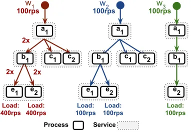
Figure 3: Example service topology, workflows in §4.1. Services are sets of processes. Workflows execute within processes, forming an execution DAG. We depict the relevant parts of the service topology separately for each workflow.

The second class of performance policies relate to managing request-level end-to-end latencies. This includes differentiated ser-vices or statically prioritizing some workflows over others (e.g., premium vs. free users, or interactive vs. background tasks) [20], or meeting end-to-end latency deadlines (user facing web-sites often need to load a page in under 100-400ms)[21,63].

3.2

Challenges

The complex request execution DAGs and lack of global visibility in the SOA setting poses unique challenges in meeting the above performance goals.

Rate limiting must account for bottlenecks end-to-end. Con-sider the services from Figure3and the three workflowsw1,w2

andw3, all of which contend at processesa1.Assume a purely local

approach where all processes rate limit according to their local bottle-necks. In this case, ifw1requests execute and timeout in overloaded e2, the work they executed (and contention they introduced) ina1, b1,c1andc2is wasted. Instead, an approach that rate limitsw1ata1

reduces wasted resourcesandincreases the throughput ofw2andw3

since more resources ina1ande2would be available. However,a1is

not aware of(i)the downstream bottlenecke2,(ii)which workflows

usee2, and(iii)the load imposed by each workflow one2. This

makes it challenging to determine rate limits for each workflow ata1.

Furthermore, as workflows contend for shared resources, their rate

limits at every hop havemutual dependenciesand therefore cannot

be tuned independently of each other.

Meeting latency deadlines requires dynamic request-specific in-formation.Scheduling requests at every process to meetend-to-end

latency guarantees is challenging due to the complex structure of execution DAGs and the inherently stochastic nature of the problem (e.g., queuing effects at each process). Specifically, achieving latency goals depends on the processing times for each workflow at every service of their execution DAGs [37]. In Figure3, ifw3has a 300ms

end-to-end deadline and requires 250ms of processing time ate2, it

only has a budget of 50ms to complete ata1andb1.

Despite myriad existing scheduling algorithms to prioritize re-quests with different performance objectives (e.g., shortest remaining

Table 1: Notation used for algorithm description

w Workfloww

s Services, defined as a set of processes

p Processp

αw

p,d Amplification factor forwfrompto processd

σw

p Admission rate ofwatp

time first (SRTF) [18] and least slack time first (LSTF) [35]), realiz-ingthese policies in a fully distributed setting remains non-trivial. These algorithms rely on information such as the remaining pro-cessing time and slack to deadlines, which need to be dynamically estimated across diverse workflows.

3.3

Design principles

Given the scale and heterogeneity of the applications we aim to support, the design of Wisp is driven by three core requirements:

(i)avoid centralized coordination,(ii)exchange minimal

informa-tion between services,(iii)operate without prior knowledge of a

workflow’s costs and graph structure. At the same time, Wisp must provide building blocks for operators to enforce flexible system-wide policies depending on their requirements with minimal tuning. These considerations led us to a design with the following key func-tionalities:

Workflow-level distributed rate adaptation.Processes use a lo-cal policy to identify admission rates for requests of different work-flows and share them with their upstream neighbors. Next, Wisp uses a novel distributed rate adaptation protocol to bubble these admission rates through the service chain, calibrating rate limiters at upstream services to account for bottlenecks downstream. This ensures that workflows are rate limited asearly as possibleinstead of only being throttled at the point of congestion (§3.2). Furthermore, we perform admission control to avoid wasting resources on requests that will not complete within their deadlines.

Request-level scheduling.Wisp leverages request schedulers at every process to mediate access to local resources. Schedulers may enforce fair queuing across requests from different workflows to guarantee performance isolation, or use policies such as shortest job first (SJF), earliest deadline first (EDF), and least slack time first (LSTF) to optimize for a range of end-to-end performance goals. Wisp dynamically estimates end-to-end properties of requests such as their remaining processing time to execute algorithms such as LSTF.

4

DESIGN

We now discuss our solutions for workflow-level distributed rate adaptation and request-level scheduling.

4.1

Workflow-level rate adaptation

Algorithm 1Rate adaptation atp∈w(every 100ms)

Constants:q: quantile parameter 1: σ_pw ←LocalResourceSharinдPolicy() 2: for allD|downstream servicesdo

3: for alld|processes in service Ddo ▷In parallel 4: σ_dw ←GetRates(d)/α_p,dw

5: σ_pw←min(σ_pw,Q(σ_dw(d∈D),q))

illustrative example in §4.1.2, and further comment on its tuning in §4.1.3.

4.1.1 Distributed rate adaptation algorithm

The goal of each processpis to set a rate limitσ_pwfor each workflow

w, to enforce a specific resource sharing policy across workflows, while balancing the system utilization and the request drop

prob-ability. Concretely, every processp, for a workfloww, computes

a rate limitσ_pw as the minimum between the local rate limit and

the rate limits of downstream services ofp.pperiodically executes

Algorithm1(see notation in Table1).

Monitoring workflow characteristics.To determine their local rate limits as well as those of their downstream services, processes re-quire information about each workloadw. Specifically, each process

pmonitors the average load on local resources by each workflow. It also maintainsαw_p,d, theamplification factorofwfrom processpto a downstream processd. For instance, in Figure3, if the measured arrival rates ata1andb1forw1are 100 and 200, respectively, then αw1

a1,b1=2; in other words, a single request ofw1ina1triggers two

requests tob1on average.

Adapting local rate limits (Line 1).Our algorithm starts withp computing its local rate limits through an operator-specified policy (§4.3). Policies observe the load on local resources by different workflows to infer theircosts(§5). They then computelocal rate limitssuch that the resulting share of each resource by a workflow corresponds to a policy (say, bottleneck fairness). As the resource share or cost forwchanges, the local rate limits adapt accordingly. In Line 1,pinitializesσ_pw to the local rate limits by executing the policy.

Trading off utilization for dropped requests (Lines 2-5). Next, for each downstream serviceD,pqueries the rate limits of the pro-cessesd ∈D, scaled by the amplification factorαw_p,d (Lines 2-4). Intuitively, ifevery processpsets itsσ_pw according to the mini-mumof its local rate limit and that of its downstream processes, we avoid overload along the service topology. However, this approach is conservative and may significantly reduce resource utilization. For example, if a process communicates with 100 downstream processes, a slowdown in one of those processes directly reduces the admission rate which then propagates upstream.

Instead of using the minimum, we propose using a quantile

func-tion Q, which depends on a quantileknobq∈[0,1](Line 5). For

example,q=0.5uses the median downstream rate and makesQ

ro-bust to outliers; however, the overloaded downstream services drop requests that are in excess of their announced rate limits. Navigating

this trade-off allows us to increase resource utilization. We discuss the tuning of the knobqin §4.1.3.

Computingσ_pw (Line 5).Finally,padjusts its announced rate

σ_pw as the minimum between the current rate and the value ofQ,

which can be regarded as theper-serviceaggregate rate (of D).p

distributes its announcedσ_pw to its upstream processes in proportion to their demands, when the upstream processes invokeGetRates(·)

(Line 4).

In summary, every iteration ofAlgorithm1bubbles up

admis-sion rates through the service topology, with processes of upstream services enforcing rate limits that account for downstream service rates according to the quantile knobq.

4.1.2 Rate adaptation trade-off by example

We now present a simple example to describe the behavior of

Al-gorithm1. Consider the setting in Figure3. The three workflows

w1,w2, andw3have an arrival rate (demand) of 100rps each ata1,

and a subsequent load at(e1,e2)of(400,400)rps,(100,100)rps, and (0,100)rpsrespectively. Assume that all processes have a capacity of 500rps each.

This implies that the total load ate2 from all three workflows

exceeds its capacity of 500rps. Assume running a max-min fairness policy ate2, which, observing the load per workflow, asserts thatw1

is exceeding its fair share of 300rps and needs to be rate limited. Withq=0,σw1

a1 is computed to be 75rps, which guarantees that

e1ande2receive 300rps of load fromw1, but thereby leaves 100rps

of spare capacity ate1. Withq =1,σaw11in turn becomes 100rps.

This maximizes utilization ate1(400rps), bute2now drops 100rps

(incident load of 400rps, and rate limit of 300rps). This is a funda-mental trade-off in the workflow rate limiting problem: calibrating end-to-end rate limits to match the slowest process of bottlenecked services risks under-utilization (q=0), whereas matching the fastest process risks wasting resources and dropping requests (q=1).

4.1.3 Guidelines for setting the quantile knob

As the advertised rates in Algorithm1are non-decreasing in the

quantile knobq, both the request drop probability and system uti-lization increase withq. Operators can leverage this property and setqto properly balance the two. Suppose that the operator wishes to minimize a weighted sum between the average request drop rate and the average unused capacity. Let us focus first on a system with a single service and a large number of processes. Assume that the advertised ratesσ_dw from Line 4 in Algorithm1are represented by a random variableX with support[0,M]and densityf(x), and also

αw

p,d=1. The goal of the quantile knobqcan be expressed in terms

of minimizing a weighted sum of residual values

h(a) := E[(a−X)1a≥X]+βE[(X−a)1a≤X]

=

Z a

0

(a−x)f(x)dx+β

Z M

a (x−a)f(x)dx.

The expectations correspond to the average drop rate and average unused capacity under some arrival rate (demand)a;1{ · }denotes

the indicator function andβis the weighting factor. Differentiating

h(a),

h′ (a)=

Z a

0

f(x)dx−β

Z M

W₁ W₂

b₁

b₁ c₁

b₁

b₁ c₁

Time

a₁

b₁ c₁

W₁

W₂

W₁ Deadline

W₂ Deadline

W₁ Deadline

W₂ Deadline Time

EDF: W₂ request misses deadline

LSTF: W₁ and W₂ meet deadline (a

1 b1 c1)

(a

1 b1)

W₁

W₂

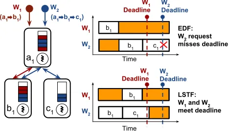
Figure 4: Scheduling example: requests fromw1andw2contend ata1

andb1. (Right) requests fromw1have a shorter deadline thanw2, but

w2requires additional processing time (atc1). (Top schedule) EDF

pri-oritizesw1atb1because of the closer deadline;w2misses its deadline.

(Bottom schedule) LSTF considers the slack forw2with progress

met-rics, and meets both deadlines.

and settingh′(a)=0, we obtain that the optimal value ofa, which

would be returned by the quantile functionQ(·)in Line 5, must

satisfyP_P(_(XX≤_≥aa)₎ =β. In the particular case whenβ=1thenais the median ofXand consequentlyq=0.5; as another example, ifβ =3

thenawould be the third quartile andq=0.75.

Now consider a more general system with a DAG ofnservices. Suppose the admission rates in each (process, service) pair are identi-cally distributed. Forβ=1, it can be shown that setting the quantile toq=0.5and using our algorithm for rate adaptation would lead to an optimal solution (the only difference in the analysis is that the differential of the weighted sum of residual values would benh′(a)); different values ofβwould lead to different optimal values ofq.

Naturally, it is hard to a-priori determine the optimal value of

qfor a general system as it depends on the distributions of the ad-mission rates of the processes for each service, and also on the distributions of the amplification factors. In fact, the operator can theoretically benefit by setting different quantile values for each (service, workflow) pair, e.g., via line-search procedure at a slow time-scale. Nonetheless, guided by the above analysis and for sim-plicity, we useq=0.5by default in our experiments (§6presents a sensitivity analysis ofq).

4.2

Request-level scheduling

While regulating the system load already improves latency, we also schedule requests at processes to further meet different performance goals. In particular, we combat stochastic effects that inflate end-to-end latencies such as bursty arrivals, and queuing at every hop.

Schedulers in Wisp enforce policies such as performance iso-lation between requests of different workflows (e.g., protect low latency workflows from head-of-line blocking due to throughput heavy workloads [20]) or prioritize their execution based on end-to-end performance objectives (e.g., meeting deadlines).

Need for estimating progress. Consider the goal of meeting end-to-end deadlines. A natural scheduling algorithm to execute at every hop is EDF, which prioritizes requests with closer deadlines. We

Table 2: Propagated metadata and components that use them (*progress metrics (§4.2)).

Metadata Used by

Workflow ID Rate limiters, fair queuing, resource

accounting

Elapsed service time * LSTF, SRTF

Total service time * LSTF

Work so far * LASF

Total work * SJF

Deadline EDF, LSTF, drop logic

discuss an execution of EDF in the context of Figure4. Requests

fromw1execute serially ata1and thenb1. Requests fromw2contend

with those fromw1ata1andb1, but additionally also execute atc1.

Atb1, requests fromw1have a closer deadline than those fromw2.

EDF in this scenario causesb1to prioritizew1overw2, eventually

causingw2to miss its deadline (Figure4, top schedule).

Algorithms such LSTF remedy this by prioritizing requests ac-cording to theirremaining processingtime and their deadline

(Fig-ure4, bottom schedule). However, Wisp by design operates

with-out prior knowledge of the costs and DAG structure of workflows. Therefore, to benefit from scheduling algorithms such as LSTF, Wisp needs to estimate metrics such as the total and the remaining process-ing time for each requestas they execute. We achieve this through

progress metrics. Note, the processing time for a request differs from its end-to-end latency (which includes waiting times). This is impor-tant, because if a request needs only 1ms of processing at a process, but the same workflow experienced 100ms of queuing delay in the past, an “expected processing time" of 100ms mischaracterizes the request’s priority for algorithms such as LSTF.

Progress metrics. We refer to metrics that reflect a request’s true

execution progress asprogress metrics. Progress metrics can be

queried for the total end-to-end estimate, elapsed, and remaining values at any point in the request execution. Example metrics we track are the processing time and total work (demand divided by capacity), which enable multiple scheduling algorithms (Table??). Every request therefore is “tagged" with the necessary progress metrics, which is updated by processes as the request executes.

algorithms that use the remaining value of a metric (e.g., SRTF and LSTF) estimate it asmtotal−melapsed at any instant.

4.3

Example operator policies

Policies to compute rate limits. Processes may choose to pro-vide static throughput guarantees, calculate rates based on bottleneck fairness, or receive feedback from the local queue schedulers and resources. As long as processes expose their per-workflow rate limits

to their upstream neighbors, the rate aggregation mechanism

trans-parentlyensures that upstream processes converge to rate limits that factor in downstream restrictions (§4.1.1). We implemented a bottle-neck fairness policy similar to [45]. With this policy, each process

pchecks if a local resource is overloaded. If not, it ramps up the

announced rate limits for every workflow for whichpis a leaf (no

further downstream services), by an additive probe factorβ, scaled according to the amount of spare capacity available (this increases the rate faster when there is spare capacity available and is conser-vative otherwise). If instead a local resource is bottlenecked, the system calculates max-min fair shares for the contending workflows.

Local scheduling policies. We now discuss multiple scheduling policies realized using our framework. We implemented a multi-resource fair queuing scheme similar to [62]. Fair queuing across workflows protects short and bursty workflows that do not benefit from rate limiting (§??). The scheduler uses the deficit round-robin

algorithm [61], wherein every workflow gets a number of credits

per-round and credits are consumed based on the expected cost of the requests. A fixed number of credits per-round are budgeted across each workflow in proportion to the shares per-workflow (com-puted via a bottleneck fairness allocation or via DRF [26]). To meet end-to-end deadlines, our LSTF policy favors requests with the least remaining slack (§??). All scheduling policies are enabled by progress metrics and other metadata propagated via the requests.

Admission control and drop policies.To regulate queue lengths system-wide (rate limiters, scheduler, and resource queues), requests need to be dropped according to different policies. For instance, a drop policy we use ensures that when a request from a workflow

warrives at a rate-limiter inp(shaping at rateσ_pw), the rate-limiter only queues a request such that it is feasible to meet the deadline. The policy computes the maximum tolerable queuing delay for a request from the request’s deadline, the average observed end-to-end

latency forwfromponwards, and the elapsed time so far. If the

expected queuing delay on the rate-limiter (inferred from the back-log) exceeds the calculated tolerance, the request is dropped. Wisp thus drops requests that have little chance of completing within their deadlines, freeing up resources for other requests. Note, typically, SOAs gracefully degrade service when sub-systems cannot service a request [12].

5

WISP IMPLEMENTATION

We find that the basic building blocks to introduce Wisp are available in most SOA frameworks [50,69,72], making it feasible to realize these ideas today. Our prototype is implemented as a C# library.

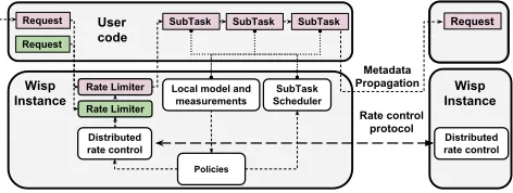
Execution model.We align our design with execution models of SOA frameworks today. Wisp comprises three components (Fig-ure5):(i)the user code which contains the business logic for the

Request

Distributed rate control

Cicero Instance

Request SubTask SubTask

Rate Limiter SubTask

Scheduler SubTask

Local model and measurements

Policies Rate Limiter

Request

User code

Wisp Instance

Request

Distributed rate control

Wisp Instance Metadata

Propagation

Rate control protocol

Distributed rate control

Figure 5: Wisp architecture. Policies examine resource utilization by different workflows locally and determine rate limiting and sub-task scheduler behavior. Distributed rate control automatically tunes up-stream rate limits to reflect downup-stream bottlenecks. Metadata prop-agation enables end-to-end scheduling policies.

application,(ii)a core that monitors workflow and resource charac-teristics, and transparently executes the distributed rate adaptation

algorithm and metadata propagation for scheduling, and(iii)the

operator specified policies that define how to compute local rate limits and scheduling decisions. Developers building micro-services

express business logic as compositions ofsub-taskstriggered by

the arrival of requests (sub-tasks are equivalent to Hystrix

com-mands[50] and Xenon tasks [72]). Rate limiting decisions are made against requests, whereas scheduling decisions are made against sub-tasks.

The core bridges user code and operator policies. As sub-tasks execute, they utilize resources such as connection pools, locks, and threadpools. Each request in Wisp has a context object propagated with it, which holds necessary metadata required for the operator policies such as the workflow ID, deadline and metrics that estimate request progress (§4.2). Furthermore, Wisp monitors utilization of the local resources and infers properties of the workflows. The meta-data propagation and local model inform resource management decisions by the operator policies (§4.3). The distributed rate adap-tation then automatically translates the constraints exposed by the rate limiting policies at each process into upstream rate limits, while

factoring in workflow characteristics (Algorithm1). The sub-task

scheduler is invoked between each execution of a sub-task, wherein it prioritizes sub-tasks based on the scheduling policies specified by the operator.

Estimating workflow and resource characteristics.The algo-rithms in §4assume the availability of some measurements at every process. This includes the arrival rates of requests per-workflow, the number of further calls per-request to downstream services (am-plification factors,α), the load per workflow per resource, and the average completion time of a workflow once admitted. We track EW-MAs of these measurements over a control interval. Furthermore, resources managed by Wisp track the load by workflow (similar abstraction as in Retro [45]). For instance, for threadpool resources, the average service time of each workflow’s task execution gives us the load. Other in-process resources such as connection pools and objects are wrapped by semaphores as in Hystrix [50] to limit con-currency, and the duration for which a workflow holds a semaphore is used to compute the load.

Front End Front

End Front End

Front End Front

End Partition Service

Front End Front

End Auth Service

Front End Front

End Extent Nodes

FE

Auth

PS

EN

A-D E F G

x400 x400 x10

x10

x10

x5

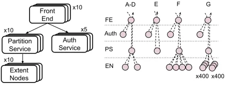
Figure 6:(Left)Azure Storagetopology used in the evaluation. Work-flows traverse four services (FE, Auth, PS andEN). Requests to a PS trigger multiple read/write sub-tasks to the ENs and local computations. (Right)Workflow DAGs in performance isolation experiment.

For instance, Finagle [69] has Broadcast Request Contexts, and

Xenon [72] hasOperation Contexts. We use similar infrastructure to not only propagate metadata in each request such as the workflow ID and end-to-end deadlines, but also to dynamically estimate request progress.

Sharing rate limits with upstream processes.In Wisp, upstream processes observe the rate limits per-workflow of their downstream neighbors in order to calibrate their own rate limits (Algorithm1). In our implementation, upstream processes directly probe their down-stream processes for their rate limits. Alternative approaches include leveraging available publish-subscribe infrastructure [56,60], or us-ing in-band mechanisms such as packus-ing rate limits per-workflow in message response headers. We leave a detailed exploration of such implementation trade-offs to future work.

6

SYSTEM EVALUATION

We now demonstrate how Wisp enforces different resource

man-agement policies:(i)Avoid overload and provide isolation in the

presence of aggressive workflows,(ii)Meet end-to-end deadlines,

and(iii)Isolate low-latency traffic from high throughput traffic. We

show(iv)how distributed rate adaptation reacts to hotspots, and

(v)how to navigate the goodput vs utilization trade-off using the

quantile knobq.

Experimental Setup.We run our experiments on a testbed com-prising forty virtual machines. Each VM has a single 2.40 GHz CPU core, 2GB of RAM and runs Windows Server 2012 R2. All services make use of the .NET CLR version 4.5. Each instance of a service in our experiments runs as a process inside a VM.

We setup a topology of services and processes according to that ofAzure Storage, discussed in §2.2; this system exhibits complex DAGs of operations, as shown in Fig.6. We reproduce request

rout-ing, execution DAGs, and sub-task cost characteristics ofAzure

Storage. Our setup comprises four tiers: front-end (FEs), authen-tication (AUTH), partition service (PS), and extent nodes (ENs). FEs are the entry points that accept client requests. FEs first verify client requests against an AUTH server. They then route requests to a PS that holds the table for a tenant, determined via consistent hashing. The PS process then issues multiple reads and writes to the EN service before executing compute work locally and returning results.

Our setup comprises ten FEs, five AUTH servers, ten PS instances and ten EN servers. Wisp monitors resource utilization by workflow

across all thread pools and connection pools in the system. For a processing stage each within the EN and PS, we vary the service times for different workflows to study different bottleneck scenarios (service times are drawn from exponential distributions). We drive client workloads from five VMs. Every workflow has a fixed number of PS partitions. Each PS partition corresponds to a fixed number of blocks on the EN tier, uniformly distributed across all EN processes. Clients generate requests according to a Poisson process [55].

Can Wisp enforce performance isolation?The workflow DAGs for this experiment are indicated in Fig.6(right). WorkflowsA-Dare read-write workloads with an arrival rate of 100rps each at the FEs. Every request from these workflows at a PS triggers a read and write request to the EN in sequence followed by some compute work at the PS. WorkflowEissues metadata queries that are serviced locally

by the PS without any interactions with the EN layer. WorkflowF

is an aggressive tenant’s workload generated by four clients that exceeds its fair share at the EN tier. WorkflowGis bursty traffic with an arrival rate of one request every two seconds, each of which triggers 400 reads in parallel, followed by 400 writes to the ENs, each of which requires a processing time of 200ms on average.

We compare performance across three scenarios:(i)Timeouts

only, where the system only makes use of deadline based timeouts and does not use fair-queuing or rate-control (baseline),(ii)rate control only (RC), and(iii)rate control and fair scheduling (FQ+RC).

Fig.7demonstrates system behavior across the three scenarios.

When workflowF, the aggressive tenant, activates at time t=50s, the resulting overload drives all workflows to throughput collapse. Given the RPC library’s request timeout of ten seconds, requests queue up internally in the system, blocking different resources and thus inflat-ing latencies for all workflows.1Instead, with Wisp’s rate-adaptation (Fig.7) this is not the case. The rate-limiting throttles workflowF

whereas other workflows retain their expected throughput. SinceF

is an open-loop workload that does not lower its sending rate despite being throttled, its throughput exhibits the instability seen in the oscillations in Fig.7(center). However, rate-control alone does not guarantee fair access to local resources at each service. This means that workflows with a stable rate have a higher degree of presence across system-wide resource queues, which cause bursty workloads

to suffer from head-of-line blocking. WorkflowGthus suffers

be-cause of the higher queue occupancies from the other workflows, indicated by a timeout fraction of 12% (Fig.7(right)). Instead, with

the combination of per-service fair-scheduling and rate-control,G

is guaranteed progress at each stage. The key take-away here is that thresholds such as timeouts are challenging to set correctly system-wide with an end-to-end performance objective in mind. In practice, such thresholds are often hard-coded [45] and therefore fragile. On the other hand, Wisp automatically adapts rate limits based on dynamic system conditions.

Can Wisp meet end-to-end deadlines?We replay a trace of 30K

requests from a production instance ofAzure Storage, which

in-volves a mix of different APIs. Since the traces do not indicate deadlines per request, we measure the completion times for each request in isolation. We then correct for the higher system loads in

1_{API timeouts for platforms such as Azure [4] and Google Cloud Platform [2] are often}

Baseline

RC

FQ + RC

40 60 80 100

10 100 1000 10000

10 100 1000 10000

10 100 1000 10000

Time (s)

Response Time (ms)

A B C D E F G Per−workflow latency

Baseline

RC

FQ + RC

40 60 80 100

0 100 200 300 400

0 100 200 300 400

0 100 200 300 400

Time (s)

Throughput (reqs/sec)

Per−workflow throughput

Baseline

RC

FQ + RC

A B C D E F G

0 25 50 75 100

0 25 50 75 100

0 25 50 75 100

Workflow

Drop Fr

action (%)

Timed out requests

Figure 7: Performance isolation experiment. (left) The median smoothed latency timeseries of the experiment shows the aggressive workflow (F, red) driving the system into overload. End-to-end rate-control throttlesFat the ingress and protects other workflows. (center) Throughput obtained by all workflows. In the baseline, all workflows’ throughputs gradually degrade as requests time out. (right) When running rate-control only, the bursty tenant is not guaranteed performance isolation as the steady workflows dominate system queues. A fair-queuing scheduler resolves this.

0 30 60 90 120

40 80 120 160 200

# Throughput Intensive Clients

Reqs/sec

Baseline Wisp

Throughput workflows, α =20

0 25 50 75 100

40 80 120 160 200

# Throughput Intensive Clients

Late Requests (%)

Baseline Wisp

Low−latency workflows

0 200 400 600

40 80 120 160 200

# Throughput Intensive Clients

A

ver

age Latency (ms)

Baseline Wisp

Low−latency workflows

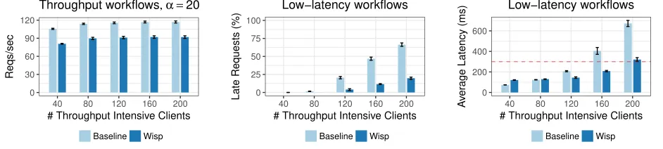
Figure 8: Average latencies and fraction of late requests for latency sensitive workflows in the presence of throughput focused clients. The low latency clients with 300ms deadlines are able to meet a high fraction of deadlines and improve average latency by 2x (200 clients).

the experiment by setting the deadline to four times the base comple-tion time when measured in isolacomple-tion. The workload includes APIs that trigger scans involvingthousandsof sub-tasks and multiple API calls that only contend for the local resource at the PS. We vary the number of client threads that generate these requests in a closed loop from 100 to 250 to increase system load.

We compare results across a baseline, FIFO+RC, EDF+RC and

LSTF+RC. Table3indicates different percentiles for the latencies

normalized by the deadline (LND). An LND of 1.0 implies that the latency equals the deadline. At higher loads, the baseline incurs increased latencies and thus misses deadlines by large factors. At the highest load of 250 clients generating requests, the baseline’s average LND is 1.33, while the 99th percentile is as high as 19.71. The improvement in LND is evident when using rate limiting (FIFO+RC), since the heavier workflows are throttled and dropped before they cause downstream congestion. With 250 clients, all algorithms with rate limiting drop close to 21% of requests since it is infeasible to meet their deadlines (§4.3), freeing up resources for other requests. We also note that LSTF outperforms EDF across all runs and yields a 10x improvement over the baseline (250 clients, 99th percentile). Recall that EDF only prioritizes requests based on the proximity to the deadline. Therefore, requests might make little progress until it is too late [14]. On the other hand, LSTFalsofactors in the remaining service time which can be estimated because of Wisp’s progress

metrics. LSTF highlights the benefits of scheduling based on end-to-end characteristics of requests using Wisp.

Can Wisp protect low-latency workflows?A common scenario in cloud storage systems is the co-existence of throughput intensive workflows which involve bulk reads/writes as well as low-latency workflows that have soft deadlines. Here, we run Wisp with the bottleneck fairness policy in conjunction with the fair scheduler. We vary the number of throughput intensive clients from 40 to 200, each of which runs in a closed loop. Every request from this workflow arriving at a PS triggers twenty sub-tasks to the EN. Six low latency clients (one workflow each) submit requests at a rate of 10 requests per-second (60 rps in total), with every request having a 300ms

dead-line. Fig.8illustrates our results. When only 40 high-throughput

clients are active, Wisp and the baseline successfully meet all dead-lines. The baseline presents an improved average latency for the low-latency clients because it does not incur the added overhead of our DRR-based fair scheduler (also observed by [62]). However, at higher loads, Wisp’s performance degrades gracefully, with a high

fraction of admitted requests meeting their deadlines (∼80% hit

rate with 200 high throughput clients). Our implementation cannot

guarantee latency for a request unless it(i)compromises on being

work-conserving or(ii)preempts on-going work at any resource

# Clients Algorithm LND LND LND (Mean) (p95) (p99) 100 Baseline 0.39 0.75 0.98

FIFO+RC 0.34 0.64 0.95 EDF+RC 0.30 0.52 0.71 LSTF+RC 0.32 0.71 0.81 150 Baseline 0.61 1.32 5.68 FIFO+RC 0.33 0.60 0.84 EDF+RC 0.31 0.52 0.69 LSTF+RC 0.3 0.51 0.71 200 Baseline 1.09 2.75 18.47

FIFO+RC 0.71 1.63 2.95 EDF+RC 0.38 0.79 1.17 LSTF+RC 0.34 0.61 0.87 250 Baseline 1.33 4.83 19.71

FIFO+RC 0.98 2.58 10.5 EDF+RC 0.49 1.25 2.15 LSTF+RC 0.46 1.12 1.82

Table 3: Mean, 95th percentile and 99th percentile latencies normalized by the deadline (LND) for requests from the production workload. An LND of 1.0 means the end-to-end latency equals the deadline.

Baseline

FIFO+RC

20 40 60 80

100 1000

100 1000

Time (s)

Response Time (ms)

A

B

C

D

Per−workflow latency

Figure 9: Skewed workload test, with a median smoothened timeseries of the latencies. WorkfowBstarts at t=40s, contends at the same PS workflowAis being routed through, and doubles its sending rate at t=60s. Wisp’s rate-limiting shieldsAfromBin both instances, without throttling background workflows (dashed, within their fair shares).

request at a service can get unlucky due to bad timing: a sub-task from a low-latency workflow may arriveright aftera burst of other workflows are scheduled (and thus suffer head-of-line blocking at the local resources). Wisp shapes the high-throughput clients to their fair share of resources alongside the low-latency clients.

Can rate adaptation react to hotspots?We now evaluate a sce-nario where we create a skewed access pattern. Four workflows activate at different times.AandBare consistently routed to the same PS, causing a hotspot on the local semaphore protected

re-source.Ais an open loop workflow generated by a single client.

Bstarts att =40swith thirty clients, and att = 60sdoubles its sending rate with an additional thirty clients joining the system. To study the rate adaptation algorithm in isolation, we only use a FIFO

scheduler at each process.CandDare background workflows that

exert pressure on the ENs. Fig.9shows a rolling median of the

latency timeseries with and without Wisp. In the baseline, whenA

140 160 180 200

0 0.5 1

Quantile (q)

TxPut (reqs/sec)

q=0 q=0.5 q=1

1000 2000 3000 4000 5000

150 200 250

150 200 250

EN

PS

FE

20 40 60 8020 40 60 8020 40 60 80 Time (s)

σ

(reqs/sec)

Figure 10:σadaptation from the ENs to the FEs for a workflow, for different values ofq. ENs adapt their rates independently based on their demands, PS’s aggregate the rates to calculate their localσusing a quantile, and the FE’s repeat the same procedure against the PS’.

activates att=40s, the surge of client requests immediately cause contention at all queues at the PS, including the shared sub-task scheduler queue as well as a semaphore being contended for. The resulting head-of-line blocking inflates latencies forB. When using

Wisp,Aexperiences a spike in latencies att = 40swhenB

acti-vates. However, whenBdoubles its sending rate att =60s, it forces head-of-line blocking and higher latencies forAas with the baseline (recall, we are not using local fair-queuing here). However, Wisp

soon computes rate limits based on the observed costs ofB. When

the rate-limiters and system queues stabilize from the unexpected surge,Aretains its expected latencies, whereasBis throttled at the entry point. Wisp also (correctly) avoids throttling the background workflows which are not contributing to congestion (and stay within their fair shares).

Quantile knob sensitivity analysis.We show the impact of the

quantile knobqof the rate adaptation mechanism. We consider

a scan workflow generated by 180 client threads, which triggers ten back-to-back requests between the PS and ENs. This workflow competes with a lighter open-loop workflow for system resources, triggering our max-min fairness policy. We study the impact of

theqon the scan workflow’s throughput. Fig.10(right) shows a

timeseries where each data point representsPσ_{(the total advertised}

rate limit) per-tier in a second for the scan workflow, for different values ofq. Withq=0, each PS selects the minimum advertisedσ from the individual EN processes, and the FEs repeat the procedure

with the PS processes. This leads to conservativeσvalues at the

FEs, leading to low utilization at the ENs. This is evident in that

(i)the EN tier probes for more demand by advertising higher rates

(Fig.10(top row, left)), and(ii)lower end-to-end throughput for the workflow (Fig.10(left)). Withq=1, the rates aremaxaggregated, and the system thus admits more work up to the ENs. This results in increased congestion at the ENs, which therefore exert back-pressure by announcing lower rates. Withq=0.5, for our setting, upstream services match the capacity of the ENs;σat FEs does not oscillate unlikeq=0andq=1, leading to a stable load at the EN (Fig.10

Overheads.In our experiments, we did not see performance over-heads from Wisp in comparison to a baseline with rate limiting and scheduling disabled (e.g., latencies in Table3and Figure9). Fur-thermore, SOA frameworks already ship with the building blocks necessary for Wisp such as rate limiters, thread schedulers and meta-data propagation. They often monitor several metrics that Wisp merely leverages to perform adaptive rate control and request sched-uling (Fig.5). For instance, Hystrix [50] already aggregates tens of metrics by “command type". Xenon [72] already performs throttling per-workflow by tenant using static rate limits.

7

DISCUSSION

Relation to auto-scaling.An alternative approach to handling

overload is to dynamically scale resources [27,54]. We believe

that scaling resources is orthogonal to Wisp’s rate control, as both approaches operate at different timescales. The former adds capacity in response to demand changes whereas Wisp regulates the demand according to the capacity. Auto-scaling typically works over slower time scales (minutes) than Wisp’s mechanisms (per-request and sub-second decisions). Furthermore, overload can be triggered by performance bugs [32,32,34] and slowdowns in third party services. Auto-scaling is not a silver bullet for these settings.

Network congestion control.Intuitively, one can view the prob-lems addressed by Wisp through the lens of network congestion control. However, the workflow rate limiting problem in SOAs dif-fers fundamentally from the network congestion control problem. In the TCP context, sources perform rate limiting and coordinate with endpoints for flow control. They infer congestion in the network either indirectly through congestion signals (e.g., packet loss and latency) or through explicit feedback [1,24] to tune their sending rates. Endpoints of a network flow are fixed (even for multicast congestion control [5]). These assumptions do not hold in an SOA. Upstream services do not know about their transitive dependencies, and due to effects such as request amplification, caching and routing, subsequent requests of the same workflow may be processed by entirely different downstream processes. Upstream services also do not know a-priori the load they impose downstream. Wisp therefore uses adaptive rate limiting and scheduling techniques that account for the unique characteristics of SOAs.

Centralized control.Finally, one may consider applying central-ized control, as in Retro [45]. However, centralized coordination hin-dersper-requestresource management (as opposed to per-workflow); e.g., scheduling decisions that account for complex workflow DAG structures. Furthermore, Retro’s approach does not see causally dis-joint request execution paths in the system, and instead, throttles

allpoints through which a workflow traverses. Instead, Wisp only

throttles a workflow along the causal path leading to a bottleneck.

Path to deployment.Wisp leverages building blocks typically available in SOA frameworks such as rate limiters, request sched-ulers and metadata propagation. The rate limiting and scheduling techniques do not depend on each other and can be used in isolation (e.g., §6demonstrates the use of rate limiting without scheduling enabled). Lastly, a system may incrementally deploy Wisp, gradually expanding the set of services that rely on Wisp for adaptive control.

8

RELATED WORK

SOA libraries. Hystrix [50] and Finagle [69] are libraries created at Netflix and Twitter to harden their production systems. They use techniques such as circuit breaking to provide resilience to failures and overload. However, they require extensive tuning of

configu-ration parameters [51], and cannot enforce multi-tenant resource

management policiesend-to-endakin to Wisp.

Admission control and latency reduction mechanisms.Trading off completeness for latency is a common approach to managing overload [37,43]. User code in Wisp can use these techniques to gracefully degrade service. [23,33,44,75] are potential admission control policies for Wisp. [59] focuses on the design of distributed rate limiters for network flows. Themis [40] manages overload for federated stream processing systems by degrading query quality fairly across users, presenting a potential rate limiting policy for Wisp.

Network flow scheduling and congestion control.Recent work has focused on resource allocation and scheduling to quickly com-plete one or multiple transfers [15,16,22], achieving low latency [9,29,36,38,76] and fair sharing networkbandwidth [42,57,58]. While they provide insights for potential Wisp policies, these spe-cific solutions do not directly apply because of differences between network flows and request execution in SOAs (§7).

Distributed systems.We discuss Retro [45] in §7as an alternative to Wisp. Pulsar [10] provides an abstraction of a virtual data center where tenants run VMs, access appliances, and a centralized sched-uler enforces rates at the level ofnetwork flows. Pulsar focuses only on throughput goals and cannot enforce request-level scheduling decisions since appliances are treated as blackboxes. Kwiken [37] considers interactive systems where requests execute in a DAG of services. However, it relies mostly on centralized resource man-agement whereas Wisp is fully decentralized. Enforcing high-level scheduling policies and fair sharing have been explored in the con-text of distributed storage systems [30,31,62,67,73,74]; however, they typically consider simpler execution structures (e.g., client to server) whereas Wisp focuses on a general DAG wherein individual processes lack end-to-end visibility. Lastly, several proposals exist for optimizing job completion times for DAGs of tasks in big-data systems [11, 28,77,78]. However, data analytics jobs are often orders of magnitude longer than those serviced by the SOA systems targeted by Wisp (which operate under the additional constraint of limited end-to-end visibility).