http://wrap.warwick.ac.uk
Original citation:Ganian, Robert , Hliněný, Petr , Králʼ, Daniel, Obdržálek, Jan , Schwartz, Jarett and Teska, Jakub . (2015) FO model checking of interval graphs. Logical Methods in Computer Science, 11 (4). 11.
Permanent WRAP url:
http://wrap.warwick.ac.uk/71266
Copyright and reuse:
The Warwick Research Archive Portal (WRAP) makes this work of researchers of the University of Warwick available open access under the following conditions.
This article is made available under the Creative Commons Attribution Non-Commercial 2.0 Licence (CC BY-ND 2.0) and may be reused according to the conditions of the license. For more details see: http://creativecommons.org/licenses/by-nd/2.0/
A note on versions:
The version presented in WRAP is the published version, or, version of record, and may be cited as it appears here.
FO MODEL CHECKING OF INTERVAL GRAPHS∗
ROBERT GANIANa, PETR HLIN ˇEN ´Yb, DANIEL KR ´AL’c, JAN OBDRˇZ ´ALEKd, JARETT SCHWARTZe, AND JAKUB TESKAf
a
Algorithms and Complexity Group, TU Wien, Favoritenstrasse 9-11, A-1040 Vienna, Austria
e-mail address: [email protected]
b,d
Faculty of Informatics, Masaryk University, Botanick´a 68a, 62100 Brno, Czech Republic
e-mail address: {hlineny,obdrzalek}@fi.muni.cz
c Mathematics Institute, University of Warwick, Coventry CV4 7AL, United Kingdom
e-mail address: [email protected]
e
Computer Science Division, UC Berkeley, 387 Soda Hall Berkeley, CA 94720-1776, United States
e-mail address: [email protected]
f Faculty of Applied Sciences, University of West Bohemia, Univerzitn´ı 8, 30614 Pilsen, Czech
Republic
e-mail address: [email protected]
Abstract. We study the computational complexity of the FO model checking problem on interval graphs, i.e., intersection graphs of intervals on the real line. The main positive result is that FO model checking and successor-invariant FO model checking can be solved in timeO(nlogn) forn-vertex interval graphs with representations containing only intervals with lengths from a prescribed finite set. We complement this result by showing that the same is not true if the lengths are restricted to any set that is dense in an open subset, e.g. in the set (1,1 +ε).
2012 ACM CCS: [Theory of computation]: Logic—Finite model theory; [Mathematics of comput-ing]: Discrete mathematics—Graph theory.
Key words and phrases: first-order model checking; parameterized complexity; interval graph; clique-width.
∗ An extended abstract of an early version of this paper has appeared at ICALP’13.
a,b,c,d,f
All the authors except for Jarett Schwartz acknowledge support of the Czech Science Foundation under grant P202/11/0196.
a Robert Ganian acknowledges support of the FWF Austrian Science Fund (X-TRACT, P26696).
e
Jarett Schwartz acknowledges support of the Fulbright and NSF Fellowships.
cThe work of Daniel Kr´al’ on the journal version of this paper was also supported by the European Research
Council under the European Union’s Seventh Framework Programme (FP7/2007-2013)/ERC grant agreement no. 259385.
b,d
The work of Petr Hlinˇen´y and Jan Obdrˇz´alek on the journal version of this paper was also supported by the Czech Science Foundation under grant 14-03501S.
LOGICAL METHODS
l
IN COMPUTER SCIENCE DOI:10.2168/LMCS-11(4:11)2015 cR. Ganian, P. Hlin ˇený, D. Král’, J. Obdržálek, J. Schwartz, and J. Teska
CC
1. Introduction
Results on the existence of an efficient algorithm for classes of problems have recently attracted a significant amount of attention. Such results are now referred to as algorithmic meta-theorems, also see a recent survey [Kre09]. The most prominent example is a theorem of Courcelle [Cou90] asserting that every MSO (monadic second order) property can be model checked in linear time on the class of graphs with bounded tree-width. Another example is a theorem of Courcelle, Makowski and Rotics [CMR00] asserting that the same conclusion holds for graphs with bounded clique-width when quantification is restricted to vertices and their subsets.
In this paper, we focus on a more restricted class of graph properties, specifically the properties expressible in first order logic. Clearly, every such property can be tested in polynomial time if we allow the degree of the polynomial to depend on the property of
interest. But is testing these properties fixed parameter tractable (FPT [DF13]), i.e. are
they testable in polynomial time where the degree of the polynomial does not depend on the considered property? The first result in this direction could be that of Seese [See96]: every FO property can be tested in linear time on graphs with bounded maximum degree. A breakthrough result of Frick and Grohe [FG01] asserts that every FO property can be tested in almost linear time on classes of graphs with locally bounded tree-width. Here, an
almost linear algorithm stands for an algorithm running in time O(n1+ε) for every ε >0.
A generalization to graph classes locally excluding a minor (with worse running time) was later obtained by Dawar, Grohe and Kreutzer [DGK07].
These results have been subsequently extended to (more general) sparse graph classes introduced by Neˇsetˇril and Ossona de Mend´ez [NdM08a, NdM08b, NdM08c]. First Dawar and Kreutzer [DK09] (also see [GK11] for the complete proof) and, independently, Dvoˇr´ak,
Kr´al’ and Thomas [DKT10], showed that every FO property can be tested in almost linear
time on classes of graphs with locally bounded expansion; examples of such graph classes include classes of graphs with bounded maximum degree or proper minor-closed classes of graphs. This series of results ultimately culminated with the recent result of Grohe, Kreutzer and Siebertz [GKS14], who established the fixed parameter tractability of testing FO properties on nowhere-dense classes of graphs (nowhere-dense being the most general class of sparse graphs).
In this work, we investigate whether structural properties of graphs that are not necessarily sparse could lead to similar results. Specifically, we study the intersection graphs of intervals on the real line, which are also called interval graphs. When restricted to unit interval graphs, i.e. intersection graphs of intervals with unit lengths, one can easily deduce the existence of a linear time algorithm for testing FO properties from Gaifman’s theorem, using the result of Courcelle et al. [CMR00] and that of Lozin [Loz08] asserting that every proper hereditary subclass of unit interval graphs, in particular, the class of unit interval graphs with bounded radius, has bounded clique-width. This observation is a starting point for our research presented in this paper.
Let us now give a definition. For a setLof reals, an interval graph is called anL-interval
graph if it is an intersection graph of intervals with lengths from L. For example, unit
interval graphs are {1}-interval graphs. IfL is a finite set of rationals, then any L-interval
graph with bounded radius has bounded clique-width (see Section 5 for further details). So,
of rationals, there existL-interval graphs with bounded radius and unbounded clique-width, and so the easy argument above does not apply.
Our main algorithmic result (Theorem 3.3) says that every fixed FO property can be
tested in timeO(nlogn) forn-vertexL-interval graphs whenLis any fixed finite set of reals
and anL-interval representation is given on the input. To prove this result, we employ a
well-known characterization of FO properties by Ehrenfeucht-Fra¨ıss´e games. Specifically, we show, using the notion of game trees introduced later, that there exists an algorithm transforming
an input L-interval graph to anotherL-interval graph that has bounded maximum degree
and that satisfies the same properties expressible by FO sentences with bounded quantifier rank. Inspired by Engelmann, Kreutzer and Siebertz [EKS12] (also see [EKK13]), we then extend our main algorithmic result to successor-invariant FO properties. We should also
mention that a recent result of Gajarsk´y et al. [GHL+15] (proven subsequently after this
work), giving a fixed parameter algorithm for testing FO properties of partial orders with
bounded width, implies Theorem 3.3 with a running time quadratic inn.
On the negative side, we show that if Lis an (infinite) set that is dense in some open
set, thenL-interval graphs can be used to model arbitrary graphs. Specifically, we show that
L-interval graphs for these sets Lallow efficient polynomially bounded FO interpretations
of all graphs. Consequently, testing FO properties for L-intervals graphs for such sets L
is W[2]-hard (see Corollary 6.2) and hence unlikely to be fixed parameter tractable. In addition, we show that unit interval graphs allow an efficient polynomially bounded MSO interpretation of all graphs and a successor FO interpretation of all graphs. So, our main algorithmic result cannot be extended to any of these two stronger logics.
The paper is organized as follows. In Section 2, we introduce the notation and the
computational model used in the paper. In the next section, we present an O(nlogn)
algorithm for deciding FO properties of L-interval graphs for finite setsL, and we extend
this result to successor-invariant FO properties in Section 4. Then, we present proofs of
the facts mentioned above on the clique-width of L-interval graphs with bounded radius in
Section 5. We finish with the several results on the interpretability of all graphs in interval graphs in Section 6.
2. Preliminaries
An interval graph is a graphG such that every vertex v of G can be associated with an intervalJ(v) = [`(v), r(v)) such that two verticesvandv0 ofGare adjacent if and only ifJ(v)
and J(v0) intersect (it can be easily shown that the considered class of graphs remains the
same regardless of whether we consider open, half-open or closed intervals in the definition).
We refer to such an assignment of intervals to the vertices of G as a representationof G.
The point `(v) is the left end pointof the interval J(v) and r(v) is itsright end point. IfLis a set of reals andr(v)−`(v)∈Lfor every vertexv, we say thatGis anL-interval
graph and we say that the representation is anL-representationofG. For example, ifL={1},
we speak about unit interval graphs. Finally, if r(v)−`(v)∈L and 0≤`(v)≤r(v)≤dfor some real d, i.e. all intervals are subintervals of [0, d), we speak about (L, d)-interval graphs.
Note that if Gis an interval graph of radiusk, thenGis also an (L,(2k+ 1) maxL)-interval
graph (we use maxL to denote the maximum element of the setL).
While an (unrestricted) interval representation of a given interval graphGcan be found
in linear time [BL76] and the same applies to unit interval graphs [CKN+95], there seem
a given L-interval graph when L is a finite set of positive reals and |L| > 1. Although, Pe’er et al. [PS97] prove that a related interval graph recognition problem in that every vertex of the input graph comes together with its prescribed interval length is NP-hard.
We thus suspect that the recognition problem of L-interval graphs might be hard in the
computational complexity sense as well and, consequently, we always assume in this paper
that an input graph comes alongside with its L-representation.
We now introduce two technical definitions related to manipulating intervals and their
lengths. These definitions are needed in the next section. IfL is a set of reals, thenL(k) is
the set of all integer linear combinations of numbers from Lwith the sum of the absolute
values of their coefficients bounded byk. For instance,L(0)={0}andL(1) =L∪(−L)∪ {0}.
An L-distanceof two intervals [a, b) and [c, d) is the smallest ksuch that c−a∈L(k). If no
such kexists, then the L-distance of two intervals is defined to be∞.
Since we do not restrict our attention toL-interval graphs where Lis a set of rationals,
we should specify the computational model considered. We use the standard RAM model with infinite arithmetic precision and unit cost of all arithmetic operations. However, we refrain from trying to exploit the power of this computational model by encoding other data in the infinite precision variables to manipulate the time complexity of the presented algorithms. In particular, we only store the end points of the intervals of the representations of input graphs and their differences in numerical variables with infinite precision and compare these values, e.g. to decide the vertex adjacencies.
2.1. Parameterized Complexity. Next we give a very brief review of the most important
concepts of parameterized complexity. For an in-depth treatment of the subject we refer the reader to other sources, e.g. [DF13].
The instances of a parameterized problem can be considered as pairshI, ki where I is
the main part of the instance andkis the parameter of the instance; the latter is usually
a non-negative integer. A parameterized problem is fixed parameter tractable (FPT) if
instanceshI, kiof size n(with respect to some reasonable encoding) can be solved in time
O(f(k)·nc) where f is a computable function and c is a constant independent of k. In
the area ofparameterized model checking, instances are considered in the form h(G, φ),|φ|i
whereGis a structure,φa formula, the question is whetherG|=φand the parameter is the
size ofφ. Therefore, when speaking about parameterized complexity of FO model checking
we implicitly consider the formula size as a parameter.
The framework of parameterized complexity offers a completeness theory, similar to the theory of NP-completeness, that allows the accumulation of strong theoretical evidence that a parameterized problem is not fixed parameter tractable. This completeness theory is based
on theweft hierarchy of equivalence classes W[1],W[2],. . . , W[P] of certain parameterized
decision problems underparameterized reductions. A parameterized reduction is an extension
of a polynomial-time many-one reduction to parameterized problems that ensures that the parameter of the new instance is bounded by a function of the parameter of the original instance. It is known that, unless the Exponential Time Hypothesis fails [IPZ01], W[1]-hard problems are not fixed parameter tractable.
parameter tractable. The parameterized FO model checking problem on general structures as well as on all graphs is AW[*]-complete [DFT96].
There exists an even stronger notion of hardness for parameterized problems: a
pa-rameterized problem is para-NP-hard if there exists a parameterk0 such that the problem
restricted to the instanceshI, k0i of parameter value equal tok0 is NP-hard.
2.2. Clique-width. We now briefly present the notion of clique-width, introduced in [CO00].
A k-labeled graph is a graph whose vertices are assigned integers (called labels) from 1 tok
(each vertex has precisely one label). The clique-width of a graphGequals the minimum k
such that Gcan be obtained using the following four operations: creating a vertex labeled 1,
relabeling all vertices with labelito labelj, adding all edges between the vertices with label
iand the vertices with label j, and taking a disjoint union of graphs obtained using these
operations.
2.3. First Order Properties. In this subsection, we introduce concepts from logic and
model theory which we use. Afirst order (FO) sentenceis a formula with no free variables
with the usual logical connectives and quantification allowed only over variables for elements
(vertices in the case of graphs). Amonadic second order (MSO) sentenceis a formula with no
free variables with the usual logical connectives where, unlike in FO sentences, quantification
over subsets of elements is allowed. An FO property is a property expressible by an FO
sentence; similarly, an MSO property is a property expressible by an MSO sentence. Finally,
thequantifier rank of a formula is the maximum number of nested quantifiers.
FO sentences are closely related to the so-called Ehrenfeucht-Fra¨ıss´e games. Thed-round
Ehrenfeucht-Fra¨ıss´e game is played on two relational structuresR and R0 (of the same type)
by two players, referred to as thespoiler and theduplicator. In each round i= 1,2, . . . d, the
spoiler chooses an element in one of the structures and the duplicator chooses an element
in the other. Let xi and yi be the elements ofR and R0 chosen in thei-th round. We say
that the duplicator wins the game if there is a strategy for the duplicator such that, for
any strategy of the spoiler, the substructure of R induced by the elements x1, . . . , xd is
always isomorphic to the substructure of R0 induced by the elements y
1, . . . , yd, with the
isomorphism mapping each xi toyi.
The following theorem [Ehr61, Fra54] relates Ehrenfeucht-Fra¨ıss´e games to FO sentences
of quantifier rank at mostd.
Theorem 2.1. Let dbe an integer. The following statements are equivalent for any two
structures R and R0:
• The structures R and R0 satisfy the same FOsentences of quantifier rank at most d. • The duplicator wins thed-round Ehrenfeucht-Fra¨ıss´e game for R and R0.
We describe possible courses of thed-round Ehrenfeucht-Fra¨ıss´e games by rooted trees.
A d-EF-tree T is a rooted tree with the following properties:
(1) each leaf v of T is associated with a relational structure S(v) with elements labelled
with 1, . . . , dsuch that each element of S(v) has at least one label (but possibly more
labels) and each label is used exactly once, and
(2) all the leaves of T are at depth d.
(1) the edges from each internal nodeu to its descendants are in one-to-one correspondence
with the elements ofR, and
(2) the structure S(v) associated with a leafv of TR is the substructure ofR induced by
the elements corresponding to the edges on the unique path from the root to v and the
element corresponding to the i-th edge of this path is labelled byi.
A mapping f from ad-EF-tree T to anotherd-EF-treeT0 is an EF-homomorphismif the
following three conditions hold:
(1) ifu is the parent of a vertex v of T, thenf(u) is the parent off(v) in T0, (2) ifu is a leaf ofT, then f(u) is a leaf ofT0, and
(3) the relational structures associated withu and f(u) are the same.
Two d-EF-trees T and T0 are EF-equivalentif there exist an EF-homomorphism fromT to
T0 and an EF-homomorphism fromT0 toT. An EF-homomorpishm that is bijective is an
EF-isomorphism.
We now formalize the connection betweend-EF-trees and Ehrenfeucht-Fra¨ıss´e games.
Theorem 2.2. Let d be an integer and let R and R0 be two relational structures. If
the full d-EF-trees of R and R0 are EF-equivalent, then the duplicator wins the d-round Ehrenfeucht-Fra¨ıss´e game for R and R0.
Proof. LetT andT0 be the d-EF-trees for R andR0, respectively, and let f :T → T0 and
f0 :T0→ T be the EF-homomorphisms witnessing their EF-equivalence. We claim that the
duplicator wins thed-round Ehrenfeucht-Fra¨ıss´e game, using the following strategy: In the
first round, if the spoiler choosesx1 inR, then the duplicator responds with y1=f(x1). If
the spoiler chooses y1 in R0, the duplicator responds with x1 =f0(y1). Assume that the
i−1 rounds of the game have been played, the elements chosen in the structures R and
R0 are x1, . . . , xi−1 andy1, . . . , yi−1, respectively, and the spoiler chooses an elementxi in
R. Letu0, . . . , ui be the path in T formed by the edges corresponding tox1, . . . , xi. The
duplicator chooses the element yi of R0 that corresponds to the edge f(ui−1)f(ui) in T0.
The definitions of full d-EF-trees and an EF-homomorphism yield that the substructures
of R andR0 induced byx
1, . . . , xi andy1, . . . , yi are isomorphic through the isomorphism
mapping xj to yj, 1≤j≤i. In particular, they are isomorphic after the drounds of the
game and the duplicator wins.
The converse implication, i.e. that if the duplicator wins thed-round Ehrenfeucht-Fra¨ıss´e
game for R and R0, then the d-EF-trees for the game played on relational structures R
and R0 are EF-equivalent, is also true. However, we omit the proof since we only need
the implication given by Theorem 2.2. We show that fulld-EF-trees can pruned to be of
bounded size.
Lemma 2.3. Consider a fixed type of relational structures. Every class of EF-equivalent
d-EF-trees contains a unique tree (up to an EF-isomorphism) with the minimum number of leaves and the number of non-EF-equivalent d-EF-trees is finite.
Proof. Let T and T0 be EF-equivalent d-EF-trees with the minimum number of leaves.
Suppose that there exists a non-bijective EF-homomorphism f from T to T0. Let f0 be
an EF-homomorphism from T0 to T. Let T00 be thed-EF-tree that is the subtree of T0
induced by the image of f. Since f is an EF-homomorphism from T toT0 andf0 restricted
to the image off is an EF-homomorphism fromT00 toT, the d-EF-tree T00 is ad-EF-tree
To show that the number of non-EF-equivalent d-EF-trees is finite, we describe the
minimal elements of EF-equivalence classes in a constructive way. Let T be a d-EF-tree.
If a vertex of T at depth d−1 is adjacent to two leaves associated with the same labelled
structure, delete one of them. The originald-EF-tree has ad-EF-homomorphism to the new
one: map all the vertices except the deleted one to themselves and map the deleted leaf to the other leaf associated with the same labelled structure. After this operation, the number
of children of any vertex at depth d−1 does not exceed the number of non-isomorphic
structures with their vertices labelled by 1, . . . , d; let K be this number. Now, if any vertex
has two children such that their subtrees are isomorphic (preserving the labelled structures
associated with their leaves), deleting one of them with its subtree results in ad-tree
EF-equivalent toT. When the pruning process stops, we have obtained the minimal d-EF-tree
EF-equivalent toT (a non-injective EF-homomorphism from ad-EF-tree always exhibits a
vertex that can be pruned in the described way).
After pruningT in the way we described, every vertex at depthd−2 has at most 2K
children, every vertex at depthd−3 has at most 22K children, etc. So, every EF-equivalence
class contains ad-EF-tree of size bounded by a function ofK and d. Clearly, there can be
only finitely many such suchd-EF-trees.
In what follows, we will refer to the minimal d-EF-tree EF-equivalent to the full d
-EF-tree of a relational structureR as the d-EF-tree of a relational structure R. Note that
thed-EF-tree of a relational structureR can be constructed from the full d-EF-tree in an
efficient way through the pruning process described in the proof of Lemma 2.3.
3. FO Model Checking
Using Theorems 2.1 and 2.2, we prove the following result for L-interval graphs.
Theorem 3.1. For every finite subset L of reals and every integer d ≥ 0, there exist
an integer K0 and an algorithm A with the following properties. The input of A is an L-representation of an n-vertex L-interval graph G and A outputs in time O(nlogn) an
L-representation of an induced subgraph G0 of G such that
• every unit interval contains at mostK0 left end points of the intervals corresponding to vertices ofG0, and
• Gand G0 satisfy the same FO sentences with quantifier rank at most d.
Proof. We are going to use Ehrenfeucht-Fra¨ıss´e games to (possibly) identify an interval
representing a vertex of Gthat can be deleted without changing the set of FO sentences
of quantifier rank at mostdsatisfied by the input graph. Hence, we first focus on proving
the existence of the number K0 and the subgraph G0 and we postpone the algorithmic
considerations to the end of the proof.
We start with perturbing the intervals to guarantee that all the left end points of the
intervals representing the vertices ofG are distinct. Choose δ to be the minimum distance
between distinct end points of the intervals in the representation. Sort the intervals by their left end points (resolving ties arbitrarily) and shift thei-th interval byiδ/2n, fori= 1, . . . , n, to the right. This does not change the graph represented by the intervals and all the end points become distinct. Note that this pertubration can be simulated by storing each end
point in the form (x, i) wherex is its original coordinate; the pair (x, i) represents the point
end-points. In this way, we can perform the perturbation in a way consistent with our computational model, i.e., without actually modifying the positions of the end points.
Chooseεto be the minimum positive element ofL(2d+2). We now establish the following.
Claim 3.2. There exists a numberK depending only on L andd such that if any interval
[a, a+δ), δ ≤ ε, contains more than K left end points of the intervals representing the vertices ofG, then Ghas a vertexw such that Gand G\ {w}satisfy the same FO sentences with quantifier rank at most d.
Fix [a, a+δ). LetI be the set of all intervals [x, x+δ) such that x−a∈L(2d+1). By
the choice of ε, the intervals of I are disjoint. In addition, the set I is finite (recall that
L is finite). Let W be the set of verticesw of G such that the left end point `(w) of the
interval corresponding tow is in an interval from I. For w∈W, leti(w) be the left end
point of the interval from I containing `(w). Define a linear order on W such that w≤w0
forw6=w0 from W if
• `(w)−i(w)< `(w0)−i(w0), or
• `(w)−i(w) =`(w0)−i(w0) and `(w)< `(w0).
We viewW as a linearly ordered set with each of its elements colored (associated) with the
pair formed byi(w) and the length of the interval of w, i.e. with elements ofI ×L. Observe
that the colors of the elements ofW (together with the linear order) determine the subgraph
of Ginduced by W.
LetK be the sum of the number of edges of all non-EF-isomorphic minimal d-EF-trees
for Ehrenfeucht-Fra¨ıss´e games played on linearly ordered sets with elements colored with
I ×L. The number K is well defined (finite) by Lemma 2.3. IfW contains more than K
elements, then there is an element w∈W such that thed-EF-trees ofW and W \ {w}are
the same, i.e. the duplicator wins the d-round Ehrenfeucht-Fra¨ıss´e game by Theorem 2.2.
Fix suchw for the rest of the proof.
We now describe a strategy for the duplicator to win thed-round Ehrenfeucht-Fra¨ıss´e
game for the graphs Gand G\w. During the game, some intervals from I will be marked
asaltered. At the beginning, the only altered interval is the interval [a, a+δ).
The duplicator strategy in thei-th round of the game is the following.
• If the spoiler chooses a vertexuwith `(u) in an interval ofI at L-distance at most 2d+1−i
from an altered interval, then the duplicator follows the winning strategy for thed-round
Ehrenfeucht-Fra¨ıss´e game for the linearly ordered colored setsW andW \ {w}. This gives
a vertexv to choose in the other graph. In addition, the duplicator marks the interval of
I that contains `(u) as altered (note that`(u) and `(v) necessarily belong to the same
interval ofI).
• Otherwise, the duplicator chooses the same vertex in the other graph and no new intervals
are marked as altered.
We now argue that the subgraphs ofG andG\wobtained in this way are isomorphic. Let
U ={u1, . . . , ud}be the chosen vertices ofG andU0 ={u01, . . . , u0d}those chosen in G\w.
Let us refer to the vertices corresponding to the intervals with left end points in the altered
intervals as altered vertices. If ui is not altered, then ui =u0i. If ui is altered, then `(ui)
and`(u0i) belong to the same intervalJ ∈ I. Suppose two vertices uj andu0j are adjacent
differently to ui than tou0i. Then `(uj) and `(u0j) belong to an intervalJ0 ∈ I atL-distance
at most one fromJ. Observe that the L-distance ofJ0 from an altered interval in thei0-th
round,i0 < i, is at most 2d+1−i0
at L-distance at most 2d+1−j in thej-th round. If j > i, thenu
j andu0j are altered because
the interval J turned to be altered in the i-th round and theL-distance ofJ and J0 is at
most one.
Since we have followed a winning strategy for the duplicator for the setsW andW\ {w},
the colors of uj and u0j are the same and they are comparable to ui and u0i in the same
way. In particular, they are adjacent to ui andu0i in the same way. We conclude that the
duplicator wins the game, which finishes the proof of the claim.
We now show that the statement of the theorem is true with K0 = Kdε−1e. The
algorithm sorts the left end points of all the intervals (this requires O(nlogn) time) and for
each of these points computes the distance to the left end of the interval that isK positions
to the right in the obtained order. If all these distances are at leastε, then every interval of
length at most εcontains at mostK left end points of the intervals and the representation
is of the desired form.
Otherwise, we chooseaandbwith the smallestb−asuch that the interval [a, b) contains
K+ 1 points and b−a < ε. By the choice of this interval, any interval of length b−a
contains at most K+ 1 left end points of the intervals from the representation. So, the
size of the d-EF-tree for the game played on the vertices v with `(v) in the intervals at
L-distance at most 2d+1 from [a, b) is bounded by a function of K, d and|L|. Since this
quantity is independent of the input graph, we can identify (in constant time) a vertex w
with`(w)∈[a, b) with the properties from the claim. We delete this vertex from the graph
G. We then update the order of the left end points and the at mostK computed distances
affected by removing w, and iterate the whole process. Storing the distances in a heap
results in an algorithm that needsO(logn) per vertex removal. Hence, the running time of
the algorithm is bounded by O(nlogn).
It is possible to think of several strategies to efficiently decide FO properties of L
-interval graphs given Theorem 3.1. We present one of them. Fix an FO sentence Φ with
quantifier rank dand apply the algorithm from Theorem 3.1 to get anL-interval graph and
a representation of this graph such that every unit interval contains at most K0 left end
points of the intervals of the representation. After this preprocessing step, every vertex of
the new graph has at most K0· dmaxLe neighbors. In particular, the maximum degree of
the new graph is bounded. The result of Seese [See96] asserts that every FO property can be decided in linear time for graphs with bounded maximum degree, and so we conclude:
Theorem 3.3. For every finite subset L of reals and every FO sentence Φ, there exists
an algorithm running in time O(nlogn) that decides whether an inputn-vertexL-interval graph Ggiven by its L-representation satisfies Φ.
4. Successor-invariant FO
A successor relation on X is simply a directed path on the vertex set X. An FO sentence
over a successor-equipped relational structure is successor-invariant if its truth does not
change when the same structure is equipped with a different successor relation. Successor-invariant FO sentences are generally more expressive than FO sentences [Ros07]. However, our previous result can be extended to this more expressive setting.
FO graph interpretation is a pair I = (ν, µ) of FO formulas ν and µ with 1 and 2 free
variables, respectively. IfGis a graph, thenI(G) is the graph such that
• its vertex set is the set of allv∈V(G) such thatG|=ν(v), and
• its edge set is the set of all the pairsu and v such thatG|=ν(u)∧ν(v)∧µ(u, v).
We require that the edge set relation as defined must be symmetric, i.e.G|= (ν(u)∧ν(v))⇒
(µ(x, y)⇔µ(y, x)) for every graph G.
Similarly, an FOsuccessor-graph interpretation is a triple I = (ν, µ, σ) of FO formulas
where ν, µ and σ have one, two and two free variables, respectively. The meaning of ν
andµis the same and σ should represent the successor relation: vis the successor of u iff
G|=ν(u)∧ν(v)∧σ(u, v). Analogously, one may also define an MSO graph interpretation
where ν and µare allowed to be MSO formulas.
A classC1of (successor-equipped) graphs has an FO interpretation in a classC2of graphs
if there exists an FO (successor-)graph interpretationI such that every (successor-equipped)
graphG1 from C1 is isomorphic toI(G2) for someG2 ∈ C2. An interpretation isefficient if
it can be computed in polynomial time. Ifh is an integer function, thenI ish-bounded if
there exists suchG2 for everyG1 with|V(G2)| ≤h(|V(G1)|). In particular, ifh is a linear
function, then we say thatI islinearly bounded and ifh is a polynomial function, then we
say that I is polynomially bounded.
Theorem 4.1. For every finite subset L of reals and every successor-invariant FOsentence
Φ, there exists an algorithm running in timeO(nlogn)that decides whether an inputn-vertex
L-interval graph Ggiven by its L-representation satisfies Φ.
Proof. The straightforward criterion [EKS12, Lemma 5.3] implies that it is enough to construct an efficient linearly bounded FO successor-graph interpretation of the class of
L-interval graphs equipped with a suitable successor relation in the class ofL-interval graphs
and apply Theorem 3.3.
Before proceeding further with the proof, we need two definitions. Two vertices in a
graph aretwins if their neighborhoods are the same. An interval representation isniceif
each interval except the last interval contains the left end point of another interval. Note that not all interval graphs have nice representations (e.g. disconnected graphs do not).
As in the proof of Theorem 3.1, we first perturb the intervals so that all their end points
are distinct. First suppose that theL-interval representation ofG is nice and letG+ be the
graph G equipped the the successor relation given by the ordering of the left end points
of the intervals. Notice that if a vertex y is the successor of a vertex x in G+, then x, y
are adjacent in G. We now construct an FO successor-graph interpretationI1 in L-interval
graphs with intervals colored black, red, green and blue.
Fix G+ and let us start with constructing the coloredL-interval graph, which we call
H. Letε >0 be such that any two end points of the intervals in the representation ofG are
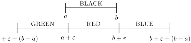
at distance larger than 3ε. For each interval [a, b), the interval representation of H contains
the following four intervals (see Figure 1):
• the black interval [a, b),
• the green interval [2a−b+ε, a+ε),
• the red interval [a+ε, b+ε), and
• the blue interval [b+ε,2b−a+ε).
Ifvis the vertex ofG+corresponding to [a, b), the four vertices corresponding to the intervals
a b BLACK
a+ε−(b−a) a+ε b+ε b+ε+ (b−a)
[image:12.612.150.469.115.187.2]GREEN RED BLUE
Figure 1: The intervals representing the four vertices ofG1 corresponding to a vertex.
We now define the interpretation I1 = (ν1, µ1, σ1). The relationsν1 and µ1 are defined
as
ν1(x)≡black(x) and µ1(x, y)≡edge(x, y). (4.1)
The definition ofσ1 is more involved. For a vertexvK ∈V(H), the red vertexvR has the
same neighborhood as vK except for the green vertex vG. Note that vR is the only red
vertex adjacent tovK with this property: indeed, any other red vertexuR adjacent tovK is
distinguished from vR by the adjacency to vB oruB. Hence, every black vertexvK can be
uniquely associated with the green vertexvG by an FO formula assoc(x, y). In particular,
assoc(x, y) holds only ifx=vK and y=vG.
If the intervals of the black vertices uK andvK intersect, then the inequality`(uK)<
`(vK) can be captured by an FO formula less(uK, vK). Specifically, this inequality can be
expressed as
less(x, y)≡ x6=y∧edge(x, y)∧ ∃zassoc(x, z)∧ ¬edge(z, y). (4.2)
The successor relation can now be interpreted using (4.2) as follows.
σ1(x, y)≡ less(x, y)∧ ∀z¬black(z)∨ ¬less(x, z)∨ ¬less(z, y) (4.3)
We now adapt the construction to the case when theL-representation of Gis not nice.
To do so, we introduce a fifth color, which we will refer to as gray. If there is an interval J
that is not the last interval and that does not contain the left end point of another interval,
we insert a gray interval J0 of length maxL that has its left end point insideJ. IfJ0 does
not contain the end point of another interval, we can shift all the intervals to the right from
J0 by the same distance in such a way that the left end point of one of them, sayJ00, moves
insideJ0 and the only new intersection we have introduced is the one between J0 and J00.
After this modification, we perform the construction described earlier, replacing each original interval with black, green, red and blue intervals and each gray interval with gray (in
the role of the black interval), green, red and blue intervals. LetH be the graph obtained in
this way. The number of black intervals in the representation ofH is the number of vertices
of G. Since there is the left end point of a black interval between the left end points of any
two gray intervals, the number of gray intervals is at most the number of black intervals. Finally, the numbers of green, red and blue intervals are the same and they are equal to the
total number of black and gray intervals. We conclude thatH has at most 8|V(G)|vertices.
It remains to adapt the FO successor-graph interpretation I1, in particular, the FO
formula σ1. The successor relation between the black intervals is again given by the order of
successor relation as follows:
σ01(x, y)≡σ1(x, y)∨ ∃zgray(z)∧σ1(x, z)∧σ1(z, y).
Observe thatH has no twins.
We now construct a FO graph interpretationI2 of five-coloredL-interval graphs with
no twins inL-interval graphs. Every gray, green, red and blue interval is replaced with two,
three, four or five identical uncolored copies; black intervals only lose their color. Let H0
be the constructedL-interval graph. Observe that the number of vertices ofH0 is at most
27|V(G)|.
Since H has no twins, the vertices ofH0 corresponding to the black intervals can be
identified by black(x)≡ ∀yx=y∨ ∃zedge(x, z)6⇔edge(y, z). In a similar way, one may
define FO formulas gray(x), green(x), red(x) and blue(x) to express that the vertex x is
one of the twins (of multiplicity two, three, four and five) corresponding to a gray, green,
red and blue interval, respectively. Combining I1 and I2, we obtain an FO successor-graph
interpretation inL-interval graphs.
5. Clique-width of Interval Graphs
Every proper hereditary subclass of unit interval graphs has bounded clique-width [Loz08] though the class of all unit interval graphs has unbounded clique-width [GR00]. In particular,
the class of ({1}, d)-interval graphs has bounded clique-width for every d > 0. Using
Gaifman’s theorem, it follows that testing FO properties of unit interval graphs can be
performed in linear time if the input graph is given by its{1}-representation with the left
end points of the intervals sorted. We generalize the result on the clique-width of unit
interval graphs for finite setsL of rational numbers, which proves a special case of our main
result for FO model checking.
Proposition 5.1. Let L be a finite set of positive rational numbers. For any d >0, the
class of (L, d)-interval graphs has bounded clique-width.
Proof. Let a be the largest rational number such that every element of L is an integer
multiple of a. Without loss of generality, we can assume that d is not a multiple of a
(otherwise, we slightly increase d). We show that the clique-width of any (L, d)-interval
graph is at mostK :=dd/ae+ 1.
LetGbe an (L, d)-interval graph with verticesv1, . . . , vnand fix an (L, d)-representation
ofG. Letbi be the smallest non-negative real such that`(vi)−bi is a multiple of a. We may
assume that all the numbersbi are distinct (by perturbing the intervals if needed). Without
loss of generality, we can also assume that 0< b1 <· · ·< bn< a.
We will now proceed in several steps. After the i-th step, we will have constructed
the subgraph ofGinduced by the vertices v1, . . . , vi such that the label of the vertexvi is
d`(vi)/ae. In the first step, we insert the vertex v1 with label d`(v1)/ae. In the i-th step,
we insert the vertex vi with label K, join it by edges to all vertices with labels between
d`(vi)/aeand dr(vi)/ae, and relabel it tod`(vi)/ae. By the choice ofaand the assumption
From Proposition 5.1 and Gaifman’s theorem, one can approach the FO model checking
problem on L-interval graphs for finite sets L of rationals. By Gaifman’s theorem, every
FO model checking instance can be reduced to model checking of basic local FO sentences,
i.e. to FO model checking onL-interval graphs with bounded radius. SinceL-interval graphs
with radius dare (L,(2d+ 1) maxL)-interval graphs and so have bounded clique-width, the
latter can be solved in linear time by [CMR00]. Combining this with the neighborhood covering technique from [FG01], which can be adapted to run in linear time in the case of
L-interval graphs given with their interval representation, we obtain the following.
Corollary 5.2. Let L be a finite set of positive rational numbers and Φ an FO sentence.
There exists a linear time algorithm that decides whether an L-interval graph Gsatisfies Φ
if the input graph G is given by itsL-representation with the left end points of the intervals sorted.
However, Proposition 5.1 is just a fortunate special case, since aside of rational lengths one can prove the following.
Proposition 5.3. For any irrationalq >0there isdsuch that the class of {1, q}, d-interval graphs has unbounded clique-width.
Proof. We may assume q > 1 (otherwise, we rescale and consider the set {1,1/q}). We
construct a {1, q}, d-interval graphG with arbitrary large clique-width kwhere d=q+ 2.
Consider a large enough integer n; the choice of n depends on k and follows from the
construction given.
We construct a sequencea1, a2, . . . , anofnpoints fromL(n)∩[0, d−1) as follows: a1 = 0, a2= 1, and for i >2 set
ai=
ai−1+ 1 if ai−1 < d−2,
ai−1−q otherwise.
The elements of the sequence defined through the latter case are calledq-elements. Informally,
we are folding a sequence of intervals of lengths one and q inside [0, q+ 1).
Choose δ > 0 such that nδ is smaller than the smallest number in L(n)∩[0, d−1).
Let us introduce the following shorthand notation: if J is an interval and r a real, then
J +r is the interval J shifted by r to the right. Similarly, if I is a set of intervals, then
I+r is the set of the intervals from I shifted byr to the right. We define sets of intervals
U1 :={[iδ,1 +iδ) : i= 0, . . . , n−1}andUq:={[iδ, q+iδ) : i= 0, . . . , n−1}. We say that
intervals [iδ,1 +iδ) and [iδ, q+iδ) areat level i.
For i= 1, . . . , n, setWi =Uq+ai ifai is aq-element ofP, andWi =U1+ai otherwise.
Observe that every interval ofWi is a subinterval of [0, d). LetG be theL-interval graph
with n2 vertices that is the intersection graph of the intervals in W1∪ W2∪ · · · ∪ Wn, and
let Wi, i = 1, . . . , n, be the vertices represented by the intervals from Wi. Finally, two
verticesx∈Wi−1 andy∈Wi, 2≤i≤n, arematesif they are represented by the same-level
intervals.
We claim that the clique-width ofGexceedskifnis sufficiently large. Suppose that the
clique-width ofGis at most k. In the construction ofGusingklabels from the definition of
clique-width, a k-labeled subgraphG1 ofGwith 13n2≤ |V(G1)| ≤ 23n2 must have appeared.
However, this implies that vertices ofG1 have at mostkdifferent neighborhoods inG\V(G1).
We will show that this is not possible.
Suppose that there existsisuch that |Wi−1∩V(G1)| − |Wi∩V(G1)|> k. Then there
have pairwise distinct neighborhoods in G\V(G1), which is impossible. Similarly, it cannot
hold that |Wi∩V(G1)| − |Wi−1∩V(G1)|> k.
In the rest of the proof, we assume that ||Wi−1∩V(G1)| − |Wi∩V(G1)|| ≤kfor every i = 2, . . . , n. We say that a set Wi is crossing if ∅ 6= Wi ∩V(G1) 6= Wi. Since we have
1
3n2≤ |V(G1)| ≤ 23n2, there exist crossing setsWi0, Wi0+1, . . . , Wi0+m wherem=bn/kc −1.
Ifn is large enough, we can select a (2k+ 1)-element subsetI ⊆ {i0, . . . , i0+m−1}such
that neitherai norai+1 is aq-element for everyi∈I (which implies thatai+1=ai+ 1) and
such that all intervals in Si∈IWi share a common point. Leti1, . . . , i2k+1 be the elements
of I ordered according to the (strictly) increasing values ofai, i.e.ai1 <· · ·< ai2k+1.
Ifj, j0∈ {1, . . . ,2k+1}andj0> j+1, then the neighborhoods of a vertex ofWij∩V(G1)
and a vertex ofWij0∩V(G1) inV(G)\V(G1) differ. Indeed, none of the vertices ofWij∩V(G1)
is adjacent to any of the vertices inWij+1+1\V(G1) while each of the vertices ofWij0∩V(G1)
is adjacent to all the vertices inWij+1+1\V(G1). Therefore, the vertices of G1 have at least
k+ 1 distinct neighborhoods inG\V(G1), which yields that the clique-width of Gis larger
thank.
6. Graph Interpretation in Interval Graphs
This section is devoted to our hardness results concerning model checking for interval graphs. We first show that Theorem 3.3 cannot be generalized to significantly wider classes of
interval graphs. To formulate our results, we need the following definition: a set Lof reals
isefficiently dense in an open setX, if there exists an algorithm that for every non-empty
open interval J ⊆X returns an element of J∩Lin time polynomial in|J|−1.
Lemma 6.1. If L is a subset of negative reals that is efficiently dense in some
non-empty open set, then there exists an efficient polynomially bounded FO interpretation of the class of all graphs in the class of L-interval graphs.
Proof. By scaling, we can assume thatL is dense in [1,1 +ε] for someε >0. LetG be a
graph with n≥2 vertices (the casen= 1 is easy to handle separately) and letv1, . . . , vn
be its vertices. We construct an FO interpretation I= (ν, µ), which is independent of the
choice ofG, and anL-interval graphH with 3n+ 5 +|E(G)|vertices such thatG=I(H).
We will describeH by giving itsL-representation. To simplify our exposition, we assume
thatL= [1,1 +ε]; it can be routinely verified that the lengths of intervals appearing in the
representation of H can be perturbed that all the length belong to a given dense subset of
[1,1 +ε]. Finally, let δ= n+1ε .
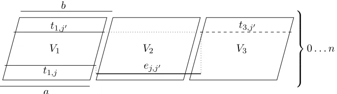
The vertex set ofH will be formed by setsV1, V2 andV3, each containing n+ 1 vertices,
a setW containing|E(G)|vertices, and two special vertices aand b. Let the vertices ofVi,
i= 1,2,3, be denotedti,j,j= 0, . . . , n, and the vertices of W be denoted ej,j0 for all pairs 1≤j < j0 ≤n such thatvjvj0 ∈E(G).
The vertices ofH are represented by the following intervals (also see Figure 2).
• The vertex ti,j,i= 1,2,3 andj = 0,1, . . . , n, is represented by the unit intervali−1 +
(1 +j)δ, i+ (1 +j)δ.
• The vertexais represented by the unit interval [0,1).
• The vertexbis represented by the unit interval(n+ 2)δ,1 + (n+ 2)δ.
V1 V2 V3
a b
t1,j
t1,j0 t3,j0
ej,j0
[image:16.612.135.477.122.218.2]0. . . n
Figure 2: The construction of the interval representation of the graph H in the proof of
Lemma 6.1.
Observe that the vertices aandt1,0 ∈V1 are twins, i.e. they have the same neighbors in H,
and that the vertexb is adjacent to every vertex inV1∪V2∪ {a} ∪W.
Note that the verticesaandt1,0 are the only twins in the graphH. In particular, they
are the only two vertices that satisfy the following formula:
anchor(x)≡ ∃y x6=y∧edge(x, y)∧ ∀z6=x, yedge(x, z)⇔edge(y, z).
We will refer to these two vertices as to the anchors. Note that the vertices of V1 are at
distance one from the anchors, those ofV2 at distance two and those of V3 at distance three
or four.
Let dist(x, y) =cfor an integer cbe the shorthand for an FO formula expressing that
the distance of two vertices x and y is c, and adist(x) =c for an FO formula expressing
that the distance ofx from an anchor is c. The vertices ofGare represented by the vertices
of V0
1 = {t1,1, . . . , t1,n}. Using this notation, the following formula is true for exactly the
vertices ofV10.
ν(x) ≡ ¬anchor(x)∧adist(x) = 1∧ ∃y(adist(y) = 2∧ ¬edge(x, y)).
Note that the last part of the formula makes ν(x) false forx=b.
In what follows, we refer to the pairs of verticest1,j and t3,j asmates. The following
formula is true if and only if x0 ∈V3 is the mate of x∈V10:
mates(x, x0) ≡ν(x)∧(adist(x0) = 3∨adist(x0) = 4)∧
∃!y adist(y) = 2∧ ¬edge(x, y)∧ ¬edge(x0, y).
Suppose thatx=t1,j andx0 =t3,j0. If j0 < j, then there exists no vertexy as in the formula
and, ifj0 > j, there exists at least two suchy’s, in particular, t2,j, . . . , t2,j0.
The vertices of V0
1 can be linearly ordered according to their left end points. This
linear order is actually reflected by dominating one vertex of another. Formally, a vertex x
dominates a vertexy ify and all its neighbors are also neighbors of x. Observe thatx∈V0 1
dominates y∈V10 if and only if the left end point ofy precedes the left end points ofx. The
following FO formula expresses that a vertexx dominates a vertexy.
Using this formula, we can define the formulaµ.
µ(x, y) ≡µ0(x, y)∨µ0(y, x), where
µ0(x, y) ≡domin(y, x)∧ ∃y0, zmates(y, y0)∧
edge(x, z)∧ ∀t(domin(x, t)→ ¬edge(t, z))∧
edge(y0, z)∧ ∀t(domin(y0, t)→ ¬edge(t, z)).
Note that µ0(x, y) for x = t1,j and y = t1,j0 is true if and only if j < j0 and the set W
contains the vertex ej,j0. Indeed,z=ej,j0 is the only possible choice of a vertex satisfying
the existential quantification.
Since the parameterized FO model checking problem is AW[*]-complete for general graphs, we can immediately conclude the following.
Corollary 6.2. If L is a subset of non-negative reals that is efficiently dense in some
non-empty open set, then FOmodel checking is AW[*]-complete on L-interval graphs when parameterized by the formula size.
We now turn our attention to interpretations in stronger logics. We start by showing that the class of all graphs has an FO interpretation in the class of unit interval graphs with a successor relation. We actually prove a stronger statement that there exists an interpretation of the class of all directed graphs.
Lemma 6.3. There exists a polynomially bounded FO interpretation of the class of all
directed graphs in the class of unit interval graphs with a successor relation.
Proof. Fix a directed graph G. Let n and m be the number of vertices and edges of G, respectively. Further, letv1, . . . , vn be the vertices ofG, letd+i andd
−
i be the out-degree and
in-degree of a vertexvi and letei,1, . . . , ei,d+
i be the edges leavingvi. We will simultaneously
describe the FO interpretationI = (ν, µ) and an unit interval graphH such that G=I(H).
For each vertexvi of G, the graphH contains the following 2 +d+i +d−i vertices: ui,
u0i andui,e for each edgee leaving or enteringvi in G. The graph H consists of ncliques,
the i-th clique formed by the 2 +d+i +d−i vertices corresponding tovi. Clearly,H is a unit
interval graph.
We now define a successor relation on the vertices ofH. To make the definition of the
successor relation less technical, we abuse the notation by writing ui,ei,0 foru
0
i (note that
there is no edge denoted byei,0 in G). The successor relation will contain the following pairs
of vertices ofH:
• (ui, u0i) = (ui, ui,ei,0) for everyi= 1, . . . , n,
• (ui,ei,j−1, ui0,ei,j) and (ui0,ei,j, ui,ei,j) for every edge ei,j, i = 1, . . . , n and j = 1, . . . , d
+ i ,
whereui0 is the head of ei,j, and • (ui,ei,d+
i
, ui+1) for everyi= 1, . . . , n−1.
Note that the only pairs of adjacent vertices included in the successor relation are those described in the first item. The following two FO formulas can be used to form the interpretation.
ν(x) ≡ ∃t succ(x, t)∧edge(x, t)
µ(x, y) ≡ ∃t, t0, t00 succ(t, t0)∧succ(t0, t00)∧
W0 W1
A A1
leveli
levelj
leveli
[image:18.612.151.466.117.200.2]levelj
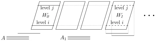
Figure 3: The interval representation of the graph H with a part representing an edgevivj
of the graphG.
It is straightforward to check that G=I(H).
Lemma 6.3 yields the following.
Corollary 6.4. FO model checking is AW[*]-complete on unit interval graphs with a
successor relation when parameterized by the formula size.
We now turn our attention to more general MSO properties. There exist two commonly
used MSO frameworks for graphs: the MSO1 language where quantifying over vertices and
vertex sets only is allowed, and MSO2 where it is allowed to quantify over edges and edge
sets in addition. Our negative result holds for the weaker variant MSO1 (and so also holds
for MSO2).
Lemma 6.5. There is a polynomially boundedMSO1 interpretation of the class of all graphs
in the class of unit interval graphs.
Proof. We describe the MSO1 interpretationI = (ν, µ). Fix an n-vertex Gwith n≥4 (the
cases with n= 1,2,3 can be handled separately in a straightforward way). Letv1, . . . , vn be
the vertices ofG ande1, . . . , em its edges. We will construct a unit interval graph H such
thatG=I(H). The graphH will be described by giving its interval representation and its
construction is illustrated in Figure 3.
Chooseδ >0 such that δn < 12 andU =[iδ,1 +iδ) : i= 0,1, . . . , n−1 . Recall that
J+xwhere J is an interval and x is a real is the intervalJ shifted by x to the right. The
graphH contains n(3m+ 1) vertices corresponding to the intervals from the sets U+k for
k= 1, . . . ,3m+ 1; the vertices corresponding to the intervals [iδ,1 +iδ) and [iδ,1 +iδ) +k
are said to be at the level i. LetW`,`= 0, . . . , m, be the set of then vertices represented
by the intervals fromU + (3`+ 1).
The graph H further contains three vertices represented by the interval [0,1) each and
mtriples of vertices represented by the intervals [0,1) + (3i−1/2),i= 1, . . . , m. The vertices
in these m+ 1 triples will be referred to asanchorsand they will be the only vertices of H
that have two twins. Also insert a vertex represented by the interval [1/2,3/2). The three
vertices represented by the interval [0,1) are the only anchors of degree four.
If the edge ek joins verticesvi and vj,H contains a pair of vertices represented by the
intervals [iδ,1 +iδ) + (3k+ 1) and [jδ,1 +jδ) + (3k+ 1). The vertices included in this step
are the only vertices ofH that have unique twins. This finishes the construction ofH.
We now give the MSO1 formulasν andµ. Let twin(x, y) be the FO formula expressing
adjacent to any of the anchors.
anchor(x)≡ ∃y, z z 6=y∧edge(z, y)∧twin(x, y)∧twin(x, z),
noanch(x)≡ ∀z anchor(z)⇒ ¬edge(x, z).
Note that the only verticesx that satisfy noanch(x) are the vertices in the sets W1, . . . , Wm
and the 2m twins corresponding to the edges of G. The vertices of G will be modeled by
the vertices of W0, which are precisely the vertices that are not adjacent to any anchor and
that are at distance two from the three anchors of degree four. In particular, the formula ν
can be chosen to be the following FO formula.
ν(x) ≡ noanch(x)∧ ∃t anchor(t)∧deg(t) = 4∧dist(t, x) = 2.
Two verticesxandx0 arematesif there exists integersp, 1≤p≤m, andi, 0≤i≤n−1,
such that one of them is represented by the interval [iδ,1 +iδ) + (3p−2) and the other is
represented by the interval [iδ,1 +iδ) + (3p+ 1). In particular, ifx∈Wp−1 andx0 ∈Wp
and the verticesx andx0 are represented by intervals at the same level, thenx andx0 are
mates. It is easy to verify that two vertices x andx0 are mates iff they satisfy the following
FO formula.
mates(x, x0) ≡ noanch(x)∧noanch(x0)∧dist(x, x0) = 4∧ ∃tanchor(t)∧
∃!y∃!z ¬edge(y, z)∧edge(y, t)∧edge(z, t)∧dist(x, y) = 2∧ dist(x0, y)>2∧dist(x0, z) = 2∧dist(x, z)>2.
The transitive closure of the binary relation given by mates can be described by the following
MSO formula mates∗(x, y).
mates∗(x, x0) ≡ x=x0∨ ∃U x∈U∧x0 ∈U∧ ∃!t∈U mates(x, t)∧
∃!t∈U mates(x0, t)∧ ∀y∈U(x6=y∧x0 6=y)⇒ (∃t∈U ∃!t0 ∈U t6=t0∧mates(y, t)∧mates(y, t0)).
Note that this is the only place in the proof where we need the expressive power of MSO.
The formula µcan now be chosen as follows.
µ(x, y) ≡ x6=y∧ ∃x0, x00, y0, y00 edge(x0, y0)∧
mates∗(x, x0)∧mates∗(y, y0)∧twin(x0, x00)∧twin(y0, y00).
Indeed, if xand y belong toW0, thenµ(x, y) is true only if there exist adjacent verticesx0
andy0 at the same level as x andy, respectively, and bothx0 andy0 have twins. However,
this happens only if the counterparts ofx and y inGare joined by an edge.
Hence we obtain the following.
Corollary 6.6. MSO1 model checking is para-NP-hard on unit interval graphs.
Note that the aforementioned result of Lozin [Loz08] states that every proper hereditary
subclass of unit interval graphs has bounded clique-width, and hence MSO1 model checking
References
[BL76] K. Booth and G. Lueker. Testing for the consecutive ones property, interval graphs, and graph planarity using PQ-tree algorithms.J. Comput. Syst. Sci., 13(3):335–379, 1976.
[CKN+95] D. Corneil, H. Kim, S. Natarajan, S. Olariu, and A. Sprague. Simple linear time recognition of
unit interval graphs.Inf. Process. Lett., 55(2):99–104, 1995.
[CMR00] B. Courcelle, J. A. Makowsky, and U. Rotics. Linear time solvable optimization problems on graphs of bounded clique-width.Theory Comput. Syst., 33(2):125–150, 2000.
[CO00] B. Courcelle and S. Olariu. Upper bounds to the clique width of graphs.Discrete Appl. Math., 101(1-3):77–114, 2000.
[Cou90] B. Courcelle. The monadic second order logic of graphs I: Recognizable sets of finite graphs.
Inform. and Comput., 85:12–75, 1990.
[DF13] R. Downey and M. Fellows.Fundamentals of Parameterized Complexity. Texts in Computer Science. Springer, 2013.
[DFT96] R. Downey, M. Fellows, and U. Taylor. The parameterized complexity of relational database queries and an improved characterization of W[1]. InDMTCS’96, pages 194–213. Springer, 1996. [DGK07] A. Dawar, M. Grohe, and S. Kreutzer. Locally excluding a minor. InLICS’07, pages 270–279.
IEEE, 2007.
[DK09] A. Dawar and S. Kreutzer. Parameterized complexity of first-order logic.Electronic Colloquium on Computational Complexity (ECCC), TR09-131, 2009.
[DKT10] Z. Dvoˇr´ak, D. Kr´al’, and R. Thomas. Deciding first-order properties for sparse graphs. InFOCS’10, pages 133–142. IEEE, 2010.
[Ehr61] A. Ehrenfeucht. An application of games to the completeness problem for formalized theories.
Fund. Math., 49:129–141, 1961.
[EKK13] K. Eickmeyer, K. Kawarabayashi, and S. Kreutzer. Model checking for successor-invariant first-order logic on minor-closed graph classes. InLICS, pages 134–142. IEEE, 2013.
[EKS12] V. Engelmann, S. Kreutzer, and S. Siebertz. First-order and monadic second-order model-checking on ordered structures. InLICS, pages 275–284. IEEE, 2012.
[FG01] M. Frick and M. Grohe. Deciding first-order properties of locally tree-decomposable structures.J. ACM, 48(6):1184–1206, 2001.
[Fra54] R. Fra¨ıss´e. Sur quelques classifications des syst`emes de relations.Universit´e d’Alger, Publications Scientifiques, S´erie A, 1:35–182, 1954.
[GHL+15] J. Gajarsk´y, P. Hlinˇen´y, D. Lokshtanov, J. Obdrˇz´alek, S. Ordyniak, M. S. Ramanujan, and S. Saurabh. FO model checking on posets of bounded width. InFOCS’15. IEEE, 2015. To appear. [GK11] M. Grohe and S. Kreutzer. Methods for algorithmic meta theorems. InModel Theoretic Methods in
Finite Combinatorics: AMS-ASL Special Session, January 5-8, 2009, Contemporary Mathematics, pages 181–206. AMS, 2011.
[GKS14] M. Grohe, S. Kreutzer, and S. Siebertz. Deciding first-order properties of nowhere dense graphs. InSTOC’14, pages 89–98. ACM, 2014.
[GR00] M. Golumbic and U. Rotics. On the clique-width of some perfect graph classes.Int. J. Found. Comput. Sci., 11(3):423–443, 2000.
[IPZ01] R. Impagliazzo, R. Paturi, and F. Zane. Which problems have strongly exponential complexity?
J. Comput. System Sci., 63(4):512–530, 2001.
[Kre09] S. Kreutzer. Algorithmic meta-theorems.Electronic Colloquium on Computational Complexity (ECCC), TR09-147, 2009.
[Loz08] V. Lozin. From tree-width to clique-width: Excluding a unit interval graph. InISAAC’08, volume 5369 ofLNCS, pages 871–882. Springer, 2008.
[NdM08a] J. Neˇsetˇril and P. Ossona de Mendez. Grad and classes with bounded expansion I. Decompositions.
European J. Combin, 29(3):760–776, 2008.
[NdM08b] J. Neˇsetˇril and P. Ossona de Mendez. Grad and classes with bounded expansion II. Algorithmic aspects.European J. Combin, 29(3):777–791, 2008.
[NdM08c] J. Neˇsetˇril and P. Ossona de Mendez. Grad and classes with bounded expansion III. Restricted graph homomorphism dualities.European J. Combin, 29(4):1012–1024, 2008.
[Rab64] M. O. Rabin. A simple method for undecidability proofs and some applications. In Y. Bar-Hillel, editor,Logic, Methodology and Philosophy of Sciences, volume 1, pages 58–68. North-Holland, Amsterdam, 1964.
[Ros07] B. Rossman. Successor-invariant first-order logic on finite structures.J. Symb. Log., 72(2):601–618, 2007.
[See96] D. Seese. Linear time computable problems and first-order descriptions.Math. Structures Comput. Sci., 6(6):505–526, 1996.