Munich Personal RePEc Archive
GMM Unit Root Inference in Generally
Trending and Cross-Correlated Dynamic
Panels
Robertson, Donald and Sarafidis, Vasilis and Westerlund,
Joakim
Monash University
5 February 2014
Online at
https://mpra.ub.uni-muenchen.de/53419/
U
NIT
R
OOT
I
NFERENCE IN
G
ENERALLY
T
RENDING AND
C
ROSS
-C
ORRELATED
F
IXED
-
T
P
ANELS
∗
Donald Robertson University of Cambridge
UK
Vasilis Sarafidis† Monash University
Australia
Joakim Westerlund Deakin University
Australia
February 3, 2014
Abstract
This paper proposes a new panel unit root test based on the generalized method of
moments approach for panels with a small number of time periods and a large number
of cross-section units,N. In the model that we consider the deterministic trend function is essentially unrestricted and the errors are cross-sectionally correlated in a very general
fashion. In spite of these allowances, the GMM-statistic is shown to be asymptotically
unbiased,√N-consistent and asymptotically normal for all values of the autoregressive (AR) coefficient,ρ, including unity, making it an ideal candidate for unit root inference.
Results from both simulated and real data are provided to suggest that the asymptotic
properties are borne out well in small samples.
JEL Classification:C12; C13; C33; C36.
Keywords:Panel data; unit root test; cross-section dependence; common factors; GMM.
1
Introduction
There is a voluminous literature on panel unit root tests. The main motivation for using such
procedures is that by considering not one but Ntime series of lengthTthe power of
panel-based tests can increase considerably relative to that achievable using univariate tests. The
largest branch of literature by far is that focusing on panels where both N andT are large
(see Breitung and Pesaran, 2008, for an overview). A typical study assumes that N, T → ∞
∗The authors would like to thank seminar participants at Monash University for useful comments and
sug-gestions.
such thatN/T→∞. The main reason for this is the presence of cross-section heterogeneity,
such as fixed effects, whose estimation requiresT → ∞. This induces an estimation error
in T, which can only be controlled if N/T → 0, for otherwise the accumulated effect as
N → ∞will be unbounded (see Westerlund and Breitung, 2013, Section 5, for a detailed
discussion). This requirement may put strain on the data. Indeed, as a large body of Monte
Carlo evidence shows (see, for example, De Wachter et al., 2007; Hlouskova and Wagner,
2006), while the large-Nrequirement is usually not a problem, the large-Trequirement, and
in particular the requirement thatTmust be larger thanN, pose a real restriction, to the point
that researchers might well find themselves discarding data in order to haveN sufficiently
small relative to T. Moreover, in many panels, such as those frequently encountered in
applied micro,T(N) is simply too small (large) for such discarding practices to make sense,
although the unit root hypothesis is still of considerable interest (see Bond et al., 2005).
The above issue has motivated researchers to look for inferential procedures that are
suit-able in fixed-T panels. Harris and Tzavalis (1999) proposed a panel unit root test based on
the bias-corrected ordinary least squares (OLS) estimator of the autoregressive (AR)
coeffi-cient,ρ. Many other tests have since then been proposed (see De Blander and Dhaene, 2012,
and the references provided therein).1The evidence reported so far (see, for example, Harris
and Tzavalis, 1999; Hadri and Larsson, 2005; Hlouskova and Wagner, 2006) suggests that in
terms of small-sample performance, not requiring T to be large can be a great advantage.
In fact, fixed-Ttests often outperform large-T tests and do so for a wide range of values of
T. However, while much progress has been made, there are still plenty of important issues
remaining unresolved in the fixed-T literature. First, except for Harris and Tzavalis (2004)
and Han and Phillips (2010), who consider the case with a linear trend, the fixed-Tliterature
has not yet ventured outside the fixed effects environment. This is noteworthy because if
one admits to the possibility that time series might be trending (in a potentially non-linear
fashion), then the probability of the panel of multiple time series exhibiting at least some
trending behavior will tend to one as N → ∞, in which case fixed effects-only tests will be
rendered invalid. Second, as far as we are aware, there is presently no test that is able to
accommodate cross-section dependence, that is, existing fixed-Ttests are “first-generation”
tests (Baltagi, 2008, Chapter 12). This is again noteworthy because in practice such
depen-dence is likely to be the rule rather than the exception, even in highly disaggregated data,
because of herd behavior, fashions or fads.
The current paper addresses both issues. We develop a “second-generation” approach
to unit roots in fixed-Tpanels characterized by both cross-section dependence and generally
trending behavior. This is accomplished by assuming that the data admits to a common
fac-tor structure in which the facfac-tors are treated as unknown parameters to be estimated along
with the other parameters of the model. This parametric treatment means that the factors are
virtually unrestricted, apart from some mild regulatory conditions. It also provides a means
to control for (unobserved) deterministic trend terms, which in our model appear naturally
as additional factors. In the terminology of Bai (2009), the model that we consider constitutes
an “interactive effects” model. Interestingly, since factors are estimated, the usual problem
in empirical work of deciding on which deterministic terms to include does not arise. Hence,
the approach is not only general, but is in this sense also remarkably simple.
The estimation is carried out by modifying the generalized method of moments (GMM)
approach of Robertson and Sarafidis (2013). The new estimator is shown to have a
num-ber of desirable properties. First, it is free from the otherwise common incidental parameter
bias. This is true not only in the conventional fixed effects case, but also in the more
gen-eral interactive effects model considered here. The reason for this is that we only require
consistent estimation of the covariance matrix of the factor loadings, and not of the loadings
themselves, thereby eliminating the incidental parameter problem. Second, the estimator
supports asymptotically normal inference for all values ofρ, including unity, and the
well-known weak instruments problem whenρis in the vicinity of unity does not emerge (see,
for example, Bun and Windmeijer, 2010). Hence, unlike most existing approaches, the
limit-ing distribution of the GMM estimator considered here is continuous and has the same rate
of consistency as ρ passes through unity (see Phillips and Han, 2010, for a similar result).
Third, the estimator and the associatedt-statistic for a unit root have excellent small-sample
properties.
The remainder of the paper is organized as follows. Section 2 presents the model and
assumptions, which are used in Section 3 to derive the GMM estimator and its asymptotic
distribution. The small-sample accuracy of the asymptotic results are evaluated using both
2
Model and assumptions
Consider the panel data variableyi,t, observed for t = 0, 1, ...,Ttime series andi = 1, ...,N
cross-sectional units. The data generating process (DGP) of this variable is assumed to be
given by
yi,t = ρyi,t−1+ui,t, (1)
ui,t = λi′ft+εi,t, (2)
whereρ ∈ R,ftis anr×1 vector of common factors withλ
i being the associated vector of
factor loadings, andεi,tis an idiosyncratic error term. The following assumptions are made,
whereFtis the sigma-field generated by{εi,n}tn=1,1T = (1, ..., 1)′ is aT×1 vector, and trA
and ||A|| = √
tr(A′A)denote the trace and Frobenius (Euclidean) norm of the matrix A,
respectively.
Assumption ERR.εi,tis independent acrossiwithE(εi,t|Ft−1) =0,∑Ni=1E(ε2i,t)/N→σε2 >0
andE(ε4i,t)<∞.
Assumption LAM.λi is a random coefficient vector such that∑iN=1E(λiλ′i)/N → Σλ, an
r×rpositive definite matrix,E(||λi||8)<∞, andE(λiεj,t) =0r×1for alli,jandt.
Assumption F.
(i) F= (f1, ...,fT)′is a non-randomT×rmatrix with full column rank;
(ii) Suppose thatρ=1. If1T is included inF, thenr >1; otherwise,r>0.
Assumption INI.yi,0 = λ′if0+εi,0, where ||f0|| < ∞ andεi,0 is independent acrossi with
E(εi,0) =0,∑Ni=1E(ε2i,0)/N →σ02 >0,E(ε4i,0)<∞, andE(λiεj,0) =0r×1for alliandj.
Assumption MOM.T(T+1)/2>1+r[T+ (1−r)/2].
Assumption EPS allows for cross-section and time series heteroskedasticity but implies
no serial correlation inεi,t, the latter of which is a very common restriction in the fixed-T
liter-ature (see, for example, Bun and Sarafidis, 2013). One way to allow for more general forms of
serial correlation is to consider more lags ofyi,t, such that the AR(1) in (1) becomes an AR(p)
the choice of instruments. This is discussed in detail in Remark 3, and then again in Section
5, where we show how to implement our approach in the presence of moving average (MA)
errors. The random loading assumption can be relaxed in a relatively straightforward way,
provided that||λi||8 < ∞and limN→∞∑iN=1λiλi′/Nis positive definite. Assumption F (i) is
standard in panel data models withTfixed (see Sarafidis and Wansbeek, 2012). We note that
theFcould also be treated as stochastic by modifying the proofs accordingly. This would not
change anything else that is of substance in the paper. As we explain in Remark 2,
Assump-tion F (ii) is needed for identificaAssump-tion ofρin the unit root case. Assumption INI implies that
the equation foryi,0 can be thought of as the reduced form equation for yi,t at period time
t = 0. Thus,f0 andεi,0are not necessarily identical to the values that would arise hadyi,0
been assumed to follow (1). Assumption MOM is important because the number of factors
needs to be small enough relative to the number of moment conditions, such that there are
enough degrees of freedom to estimate the model.
A major difference when compared to the existing large-Tsecond-generation panel unit
root literature (see, for example, Bai and Ng, 2004; 2010; Moon and Perron, 2004) is that here
ft is treated as a fixed parameter vector to be estimated along with the other parameters of
the model. Whetherfthas zero mean is therefore not an issue. It can also have arbitrary
“dy-namics”. In terms of the terminology of Bai (2009), (1) and (2) constitute a fixed interactive
effects model, which is more general than the models considered previously in the literature.
Suppose, for example, thatft= (1,τt)′andλi = (ηi, 1)′, such thatλ′ift= ηi+τt. This means
that the DGP reduces to
yi,t =ρyi,t−1+ηi+τt+εi,t.
This is the benchmark first-generation specification with incidental intercepts and
time-specific fixed effects to account for cross-section dependence (see, for example, Im et al.,
2003; Levin et al., 2002). Models with incidental trends and second-generation models with
common factors can also be accommodated. For example, ifft = (1,t,g′t)′, wheregt is an
(r−2)×1 vector of common factors, andλi = (ηi,βi,δ′i)′, then
yi,t =ρyi,t−1+ηi+βit+δ′igt+εi,t.
This specification is similar to those considered by, for example, Moon and Perron (2004),
Pesaran (2007), and Phillips and Sul (2003) in the large-Tcase, and we will consider it again
this is by no means a restriction; the interactive effects model considered here can
accom-modate virtually any trend function that is linear in parameters, including polynomial trend
functions, trigonometric functions and models of discrete and smooth structural shifts. The
model considered forftis therefore very general indeed.
Moreover, while not necessary, the elements offtmay be unknown. As we illustrate in
Section 5, this means that the researcher is spared from the problem of having to decide on
which deterministic components to include. For example, if structural shifts are present,
then there is no need for any a priori knowledge regarding their locations, which are
ob-tained as part of the estimation process. Hence, not only is the model very general, but the
way thatftis accommodated is also very convenient from an empirical point of view.
Remark 1. In this paper we assume that ft enters via ui,t. This is not necessary. As Bai
and Ng (2010) discuss, when ft is random a more general DGP is obtained by placing the
common component directly underyi,t, such thatyi,t= λi′ft+ui,t, and then allowftandui,t
to have different dynamics. However, since in this paperftis fixed, the dynamics are driven
by the idiosyncratic component only, and from this point of view it does not matter whether
ftenters viaui,toryi,t.
3
Main results
3.1 Moment conditions
Define theT×Tmatrix
M = lim
N→∞
1
N N
∑
i=1Mi,
whereMi = E(y0iy′i),y0i = (yi,0, ...yi,T−1)′ andyi = (yi,1, ...yi,T)′are bothT×1. We begin by
deriving an expression forMin terms of the parameters of the DGP. This will then be used
as a basis for formulating our moment conditions. Let us begin by defining theT×T lag
matrix L=
0 0 0 . . . 0
1 0 0 . . . 0
0 1 0 . .. ...
..
. . .. ... ... 0
0 . . . 0 1 0
and theT×1 vectoret = (0, ..., 0, 1, 0, ..., 0)′, where the one is at positiont. The model foryi,t
can now be written in vector form as
yi =ρe1yi,0+ρLyi+Fλi+εi, (4)
or
yi =ρΓe1yi,0+ΓFλi+Γεi, (5)
whereεi = (εi,1, ...,εi,T)′isT×1,
Γ= (IT−ρL)−1=
1 0 . . . 0
ρ 1 . .. ...
..
. . .. ... 0
ρT−1 . . . ρ 1
,
and recall thatF = (f1, ...,fT)′ isT×r. Note thatΓis a function ofρ. In order to emphasize
this, whenever appropriate we writeΓ = Γ(ρ). By using Assumption INI to substitute for
yi,0in (5), and then stackingyi,0andyi, we obtain
[
yi,0 yi
]
=
[
1 01×T
ρΓe1 Γ
] [
f′0 F
]
λi+
[
1 01×T
ρΓe1 Γ
] [
εi,0
εi
]
.
For later use we also defineF+ = (f0,F′)′, a (T+1)×r matrix. Note that, since ρΓe1 =
(ρ,ρ2, ...,ρT)′, the matrix
[
1 01×T
ρΓe1 Γ
]
is of the same form asΓ, but of dimension(T+1)×(T+1)instead ofT×T. Hence, letting
ε0i = (εi,0, ...,εi,T−1)′ andF0= (f0, ...,fT−1)′, the following expression fory0i is obtained:
y0i =ΓF0λi+Γε0
i. (6)
Note also that in this notation,e1yi,0+Lyi = y0i, suggesting that (4) may be written as
yi =ρy0i +Fλi+εi. (7)
Let us now considerM. Substitution of (7) yields
Mi = E(y0iy′i) =E[yi0(ρy0i +Fλi+εi)′] =ρMi,−1+E(y0iλi′)F′+E(y0iε′i),
whereMi,−1 =E[y0i(y0i)′]. By using, in turn, (6) to substitute fory0i, and then the fact thatε0i
andλi are uncorrelated,E(y0iλ′i)may be written as
E(y0iλ′i) =E[(ΓF0λ
Moreover, sinceE(yi,sεi,t) =0 for alls ≤t−1 andt=1, ...,T, we have
E(y0iε′i) =
0 0 . . . 0
E(yi,1εi,1) 0 . .. ...
..
. . .. . .. 0
E(yT−1εi,1) . . . E(yT−1εi,T−1) 0
.
This matrix containT(T+1)/2 zeroes. These are our moment conditions. A natural way of
writing these conditions is as follows:
vech(M′)−ρvech(M′−1)−vech[FΣλ(F0)′Γ′] =0
T(T+1)/2×1, (9)
whereM−1is defined similarly toM, and vech is the half-vec operator that when applied to
a matrixAeliminates all supradiagonal elements ofAfrom vecA.
Unfortunately, the formulation in (9) is not very convenient to work with. Let us
there-fore denote bySt (t = 1, ...,T) theMt×Tselection matrix of zeroes and ones that picks out
the t entries of y0i which are valid at period t, that is, St is such that E[(Sty0i)εi,t] = 0t×1.
Under Assumption EPS, we have St = (It,0t×(T−t)), a t×T matrix. Hence, at time t the
vector of valid instruments is given by (yi,0, ...,yi,t−1)′. Define the T(T+1)/2×T2 matrix
S=diag(S1, ...,ST). The matrix of instruments can now be written as
Z′i = S(IT⊗y0i), (10)
which is T(T+1)/2×T. Note that Fλi = (IT ⊗λ′i)vec(F′). By using this result,
pre-multiplication of (7) byZ′i, and then taking expectations, we obtain
E(Z′iyi) =ρE(Z′iy0i) +E[Z′i(IT⊗λ′i)]vec(F′).
Combining (8) with (10), and using the fact that vec(F′) = (I
T⊗F′)e, the moment condition
in (9) can be written alternatively as
m−ρm0−S(IT⊗ΓF0ΣλF′)e=0T(T+1)/2×1, (11)
wherem= E(Z′
iyi) =vech(M′)andm0 =E(Z′iy0i) =vech(M′−1).
Remark 2. The moment condition in (11) hold for all values ofρ, provided that it is finite.
This is in contrast to many of the existing GMM estimators of dynamic panel data models
1991), which are known to suffer from a weak instrument problem whenρ≈1 (see Blundell
and Bond, 1998). To appreciate this, suppose thatT =3,ρ ∈ [0, 1],r =1 and thatft = ftis
known. In this case,f= (f1,f2, f3)′,f0= (f0,f1,f2)′and
M=
m01 m11 m21
m02 m12 m22
m03 m13 m23
, M−1 =
m00 m10 m20
m01 m11 m21
m03 m12 m22
,
suggesting that (11) can be written as
m01 m02 m12 m03 m13 m23 −ρ m00 m01 m11 m02 m12 m22
−σλ2
∑0j=0ρjfjf1
∑0j=0ρjf jf2
∑1j=0ρjfjf2
∑0j=0ρjfjf3
∑1j=0ρjf jf3
∑2j=0ρjfjf3
. (12)
Making use of the fact thatyi,t= λi∑tj=1ρjft−j+∑tj=1ρjεi,t−j, we can show that witht≥ s
mst= E(yi,syi,t) =σλ2
s
∑
j=1t
∑
n=1ρj+nfs−jft−n+σε2
s
∑
j=1ρt+s−2(j−1),
where σ2
λ is the scalar version ofΣλ and the second term on the right-hand side is equal to
ρt−s(1−ρ2(s+1))/(1−ρ2)forρ < 1 and(s+1)forρ = 1. It follows that, regardless of the
value ofρ, there is enough variation across the rows in (12) to identify the unknown
parame-ters,ρandσλ2. In the fixed effects case, however, ft =1 and therefore∑sj=1∑tn=1ρj+nfs−jft−n
reduces to(1−ρt)(1−ρs)/(1−ρ)2forρ<1 and(s+1)(t+1)forρ=1. Thus, in this case
ρandσ2
λ are identified only forρ < 1, because when ρ = 1 all rows in (12) become linear
combinations of the first row, and so there is effectively a single informative moment
condi-tion based on which it is not possible to identify two parameters. In practice, fixed effects
only are rather restrictive and, as acknowledged in the panel unit roots literature, unlikely to
be able to capture all unobserved heterogeneity in the data (see, for example, Baltagi, 2008,
Chapter 12).
Remark 3. The moment conditions in (11) can be modified to allow for error serial
corre-lation, or an AR(p) foryi,t. The case with MA errors is particularly easy. Suppose thatεi,t
follows a MA(q) process. This case can be accommodated by settingZ′i =S(IT⊗yqi), where
yqi = (yi,0, ...,yi,T−1−q)′ and thet-th diagonal element ofSis given bySt = (It,0t×(T−t−q)),
q ∈ {1, 2}. Consider next the case whenεi,t is serially uncorrelated but thatyi,t follows an
AR(2) process;
yi,t =ρ1yi,t−1+ρ2yi,t−2+ui,t,
where we assume for notational simplicity thatyi,0andyi,−1are observed. This can be
writ-ten in vector form as
yi =ρ1Γe1yi,0+ρ2Γ(e1yi,−1+e2yi,0) +ΓFλi+Γεi,
whereΓ = (IT −ρ1L−ρ2L2)−1 andL2 = LL. Alternatively, sincee1yi,0+Lyi = y0
i, with
y−i 1= e1yi,−1+e2yi,0+L2yi,
yi = ρ1y0i +ρ2y−i 1+Fλi+εi.
In this case, the matrix of instruments, Z′i, is still given by (10) but with y0i replaced by
(yi,−1,yi,0, ...,yi,T−1)′ and St = (It+1,0(t+1)×(T−t)), a (t+1)×(T+1) matrix. Thus,
pre-multiplying the expression above byZ′i, taking expectations, and then rearranging yields
m−ρ1m0−ρ2m−1−S(IT⊗ΓF−1ΣλF′)e= 0(T+T(T+1)/2)×1, (13)
wherem−1=E(Z′
iy−i 1)andF−1 = (f−1,f0, ...,fT−1)′.
3.2 Inference when F+is known
Define θ = [ρ,(vechΣλ)′]′ = (θ1,θ′
2)′ and denote by θ0 andρ0 the true values ofθand ρ,
respectively. The GMM estimator of this parameter vector, whose dimension is (1+r(r+
1)/2)×1, is given by
ˆ
θ=arg min
θ∈CθQ(θ), whereCθ is a compact subset ofR1+r(r+1)/2and
Q(θ) = g(θ)′g(θ),
g(θ) = W1/2[mˆ −ρmˆ0−S(IT⊗ΓF0ΣλF′)e],
with ˆm= ∑iN=1Z′iyi/N, ˆm0=∑iN=1Zi′y0i/N, andW= (W1/2)′W1/2is aT(T+1)/2×T(T+
1)/2 positive definite weight matrix. ˆθis the joint GMM estimator of θ1 andθ2. However,
objective function, as is commonly done in the maximum likelihood literature. The GMM
estimator ofθ2givenρis derived in (A6) and is given by
ˆ
θ2= θˆ2(ρ) = [R(ρ)′R(ρ)]−1R(ρ)′W1/2(mˆ −ρmˆ 0),
where R(ρ) = W1/2(e′⊗S)(I
T⊗KT2 ⊗IT)[vecIT ⊗(IT ⊗Γ(ρ))(F⊗F0)Dr], KT2 is the
T2×T2 commutation matrix such that KmpvecA = vecA′, where A is m×p, and Dr is
ther2×r(r+1)/2 duplication matrix such that vecB = DrvechB, whereB isr×r. The
concentrated objective function, henceforth denoted asQC(ρ), is obtained by replacingθ2in
g(θ)with ˆθ2, that is,
QC(ρ) =gC(ρ)′gC(ρ),
wheregC(ρ) =g(ρ, ˆθ2(ρ)). The estimator ofρis given by
ˆ
ρ =arg min
ρ∈Cρ
QC(ρ). (14)
whereCρis a compact subset ofR.
Assumption IDE.
(i) ρ0∈ Cρ;
(ii) g(ρ)is continuous inρandE[g(ρ)] =0(1+r(r+1)/2)×1impliesρ=ρ0;
(iii) Σg
C = limN→∞NE[gC(ρ0)gC(ρ0)′] andγ1 = limN→∞∂gC(ρ0)/∂ρ are finite with ΣgC positive definite.
Theorem 1 provides the asymptotic distribution of ˆρ.
Theorem 1.Under Assumptions EPS, LAM, F, INI, MOM and IDE, as N →∞
√
N(ρˆ−ρ0)→d N(0,σρ2),
where→d signifies convergence in distribution andσρ2= γ′1ΣgCγ1/(γ′1γ1)2. Analytical expressions
forΣg
Candγ1are given in Appendix.
Remark 4. According to Theorem 1 there is no asymptotic bias, despite the generality of the
DGP considered; (ρˆ−ρ0)is centered at zero even when scaled by
√
N. The reason for this
is no need to estimateλ1, ...,λNthemselves. This means that the number of parameters that
needs to be estimated is substantially reduced, fromNr tor(r+1)/2, thereby eliminating
the incidental parameter problem (see Bai, 2013, for a similar approach).
Remark 5.Theorem 1 holds for all values ofρ0, and in this sense it presents a unified
asymp-totic result for the GMM estimator. This is in contrast to the existing literature, in which the
asymptotic distribution of estimators depends critically on whether |ρ0| < 1, ρ0 = 1 or
indeedρ0 > 1. In fact, the only exceptions known to us are the GMM estimators of Han
and Phillips (2010), and Kruiniger (2007, 2009, 2013), which have limit distributions that are
continuous forρ0 ∈(−1, 1], but not forρ0>1.
An analytical expression forγ1is given in the Appendix. Define ˆσρ2=γˆ′1ΣˆgCγˆ1/(γˆ′1γˆ1)2,
where ˆΣg
C = NgC(ρˆ)gC(ρˆ)′ and ˆγ1 = ∂gC(ρˆ)/∂ρ. The GMMt-statistic for testingH0 :ρ0 =
ρ0is given by
t(ρ0) =
√
N(ρˆ−ρ0)
ˆ
σρ ,
and is the same regardless of the value of ρ0. The local power oft(ρ0)is easily worked out
using Theorem 1. Indeed, suppose that
ρ0= ρ0+ √c
N, (15)
wherec∈ R, such thatρ0is local toρ0, the hypothesized value under the null. In this case,
since ˆσρ2=σρ2+op(1), we can show that
t(ρ0) =
√
N(ρˆ−ρ0)
ˆ
σρ
+
√
N(ρ0−ρ0)
ˆ
σρ
d
→ N(0, 1) + c
σρ
asN →∞. Summarizing this, we have the following corollary to Theorem 1.
Corollary 1.Under (15) and the conditions of Theorem 1, as N→∞
t(ρ0)→d N(0, 1) + c
σρ.
Remark 6. Corollary 1 nests the asymptotic results under both the null and the local
alter-native hypotheses. On the one hand, ifc= 0, thenH0is true and thereforet(ρ0)→d N(0, 1).
If, on the other hand,c ̸= 0, such that the local alternative is true, then the asymptotic
consistent under the local alternative when|c/σρ| → ∞. The extent of power is driven by
two parameters, cand σ2
ρ; the smaller the uncertainty regarding ρ0 and the larger the
de-viation from the hypothesized value ofρ0, the larger the power, as expected (see Madsen,
2010, for a similar finding for some existing tests). What is unexpected, however, is the fact
that the appropriate rate of shrinking of the local alternative is the same regardless of the
specification of the deterministic trend part offt(see Han and Phillips, 2010, Section 5.2, for
a similar discussion).
Remark 7.The asymptotic distribution of most (if not all) unit root statistics depends on the
deterministic specification of the fitted test regression, which need not be equal to the true
one. In time series, this implies that different deterministic specifications have their own
critical values, whereas in panels, it implies that different specifications have their own mean
and variance correction factors (see Westerlund and Breitung, 2013, Section 3). Corollary 1
shows how the GMM-basedt-statistic has the unique and practically very useful property
that it is asymptotically invariant toF, and hence to any trend function that it may contain.
The standard fixed effects assumption is therefore not needed and the otherwise so common
mean and variance correction factors reflecting the chosen deterministic specification can be
completely avoided.
In (A7) in Appendix we show that
gC(ρ) =P(ρ)W1/2(mˆ −ρmˆ0),
where P(ρ) = IT(T+1)/2−R(ρ)[R(ρ)R(ρ)′]−1R(ρ)′. This formulation of gC(ρ) suggests a
simple estimation approach that can be used also whenFis unknown. In particular, while
nonlinear inρ, withWandF+known,R(ρ)does not depend on any other parameters that
are unknown. Hence, assuming for a moment that alsoρ is known, then so is R = R(ρ),
in which case QC(ρ) is just the (weighted) sum of squared residuals, and therefore the
GMM estimator ˆρ is just the (weighted) OLS slope estimator in a regression of PW1/2mˆ
ontoPW1/2mˆ 0:
ˆ
ρ= ρˆ(P) = (mˆ
0)′(W1/2)′P′PW1/2mˆ (mˆ0)′(W1/2)′P′PW1/2mˆ0,
where P = P(ρ0). Although Pis not observed when estimating ρ0, and vice versa, we can
we are interested in testingH0: ρ0= ρ0. A natural initialization forρin this case is given by
ρ=ρ0. The GMM estimator ofθ
2can then be obtained as ˆθ2(ρˆ).
3.3 Inference when F+is unknown
For F+ is unknown we define θ = [ρ,(vechΣλ)′,(vecF+)′]′ = (θ1,θ′
2,θ′3)′, which is (1+
r(r+1)/2+ (T+1)r)×1. The estimation of this parameter vector can also proceed in
an iterative fashion, as before. The only difference is that since nowF+ is unknown, even
if ρ was known, R and hence alsoP would still be unknown. In order to emphasize this
dependence on F+ we write P(ρ,F+) for P. The estimator ˆF+ of F+ may be obtained as
follows:
1. Initializeρ.
2. The lastTrows of ˆF+can be obtained as the eigenvectors corresponding to therlargest
eigenvalues of theT×T matrix∑Ni=1(yi−ρyi0)(yi−ρy0i)′/N. The first row of ˆF+can
be obtained as the first observation of each of the eigenvectors corresponding to ther
largest eigenvalues of∑iN=1y2i,0/N. Write ˆF+(ρ)for ˆF+.
3. The estimator ofρis given by ˆρ(P)ˆ , where ˆP= P(ˆ ρ) =P(ρ, ˆF+(ρ)).
4. Update ˆF+(ρˆ), ˆP(ρˆ)and ˆρ(P)ˆ . Repeat until convergence.
Remark 8. So far we have assumed that the number of factors,r, is known. However, the
asymptotic results also hold whenris replaced by a consistent estimator, ˆrsay. Write ˆρ(P,r)
for ˆρ. To see that ˆρ(P, ˆr)has the same asymptotic distribution as ˆρ(P) =ρˆ(P,r), consider
P(√N[ρˆ(P, ˆr)−ρ0]≤δ) = P(√N[ρˆ(P, ˆr)−ρ0]≤δ|rˆ= r)P(rˆ =r)
+ P(√N[ρˆ(P, ˆr)−ρ0]≤δ|rˆ̸=r)P(rˆ̸=r).
BecauseP(rˆ= r)→1 andP(rˆ ̸=r)→0, the second term on the right-hand side converges
to zero, and P(√N[ρˆ(P, ˆr)−ρ0] ≤ δ) =1+o(1). Moreover, conditional on ˆr = r, ˆρ(P, ˆr) =
ˆ
ρ(P,r). Thus,
|P(√N[ρˆ(P, ˆr)−ρ0]≤δ)−P(
√
Ahn et al. (2013) consider the problem of consistent estimation ofrin the context of a static
panel data regression with factors, and make several suggestions toward this end. It is
con-jectured that these estimators are consistent also in the present setup. In Section 4 we
exam-ine the performance of our GMM approach when combexam-ined with BIC1 information criterion
of Ahn et al. (2013).
4
Monte Carlo simulations
4.1 Design
The DGP is given by a restricted version of (1) and (2). Two specifications ofεi,tare
consid-ered. In the first,εi,t ∼ N(0, 1), whereas in the second,εi,tis generated as an MA(1) process;
εi,t = vi,t+φvi,t−1, wherevi,t ∼ N(0, 1/(1−φ2))andφ = 0.7. The common component is
specified withλi = [ηi,βi(1−ρ0),δ′i]′ andft = (1,t,g′t)′, such that
yi,t =ρ0yi,t−1+ηi+βi(1−ρ0)t+δi′gt+εi,t.
Heregt ∼ N(0r0×1,Ir0)is anr0×1 vector of unobserved common factors with loadingδi ∼
N(0r0×1,σ
2
δIr0), wherer0 ∈ {1, 2}andσδ2 ∈ {0.5, 2.5}. Whenσδ2 = 0.5 the proportion of the
variance ofui,tthat is due to variations inδi′gtis 33%, whereas whenσδ2=2.5 this proportion
is 72%. The intercept and trend slope,ηi andβi, are both drawn fromN(0, 1). Hence, in this
DGP, while under the unit root null (ρ0 = 1),yi,t follows a random walk with drift, under
the alternative thatρ0 ∈ {0.95, 0.99},yi,t is trend stationary.2 Finally,yi,0 = ηi+ui,0, where
ui,0 ∼ N(0, 1). We setT = 8 andN ∈ {100, 400, 1600}. All experiments are based on 2000
replications.
4.2 Results
Two versions of our estimator are simulated, both based on (14). The first, denoted GMM1,
is the one-step estimator that makes use ofW =IT(T+1)/2, while the second, GMM2, makes
use of the optimal weighting matrix, that is,W = Σˆg
C. In both cases, the number of
un-known factors,r0, is estimated using the BIC1 criterion of Ahn et al. (2013), which is of the
form BIC1= J−penalty, whereJdenotes the value of the Hansen–Sargan statistic for
overi-dentifying restrictions and the exact form of the penalty is given in Ahn et al. (2013). The
2We also considered the case whenλ′
ift =ηi(1−ρ0) +δ′igt; however, since the results were very similar, we
maximum number of factors considered is set tormax = r0+1. The following results are
reported: (i) mean, standard deviation (SD) and root mean squared error (RMSE) for GMM1
and GMM2; (ii) size (nominal size is 5% ) and power of t(1) for the unit root t-statistic;
(iii) the 5% size of the J-statistic for overidentifying restrictions, which is only relevant for
GMM2; (iv) the correct selection frequency for BIC1 (based on GMM2).
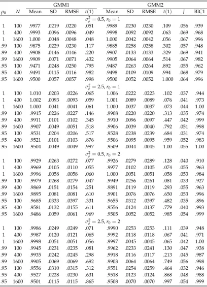
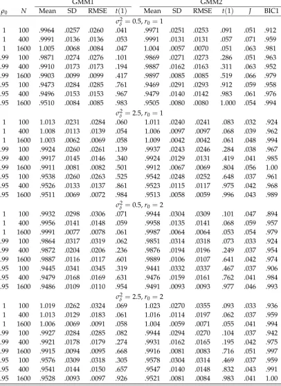
Table 1 contains the results for the case whenεi,t ∼ N(0, 1). In this case, since there is
no error serial correlation, the full set of T(T+1)/2 = 36 moment conditions is used. It is
seen that the performance of the estimators and their t-statistics is more than satisfactory.
In particular, the bias is small and it get closer to zero as Nincreases. As expected, unless
N = 100, GMM2 is more efficient than GMM1. We also see that the size of the J-statistic is
close to the nominal 5% level. This is reflected in the results for BIC1, which is very accurate.
In fact, the correct selection frequency does not fall below 90% except one instance.
The size of thet(1)-statistic is close to the nominal level in all experiments considered.
The only exception is when N = 100, in which case the GMM2-based statistic is oversized;
however, the distortions vanishes rapidly as Nincreases. The highest power is obtained by
using the GMM2-basedt(1)-statistic, which is to be expected given that GMM2 is relatively
more efficient. Naturally, the power of both statistics increases asρ0deviates from unity and
asNincreases.
Larger values of σ2
δ are generally associated with increased performance; GMM1 and
GMM2 tend to become more accurate, and the size accuracy and power of t(1)improves.
This is because a largerσδ2will make the common component easier to discern. Larger values
of r, on the other hand, tend to push the results in the other direction, that is, performance
is decreasing in the number of unknown factors. This latter effect is in accordance with our
expectations, as the number of parameters increases while the information contained in the
data (number of moment conditions) stays the same.
5
Application
5.1 Gibrat’s law
In this section we make use of our methodology in order to examine the empirical validity of
the well known “law of proportionate effect”, or simply “Gibrat’s law” (Gibrat, 1931) using
independent of their initial size. The model is the same as in (1), whereyi,tis now the size of
firmiat timetin logs. It is instructive to rewrite this model as
∆yi,t = (ρ0−1)yi,t−1+ui,t.
For ρ0 < 1 larger firms tend to grow at a lower rate compared to smaller firms, while for
ρ0 > 1 the process is explosive and growth rate is proportional to firm size. For ρ0 = 1
Gibrat’s law holds true because firms’ growth rate is independent of their initial size. An
advantage of our methodology is that it remains valid throughout the range of possible
values ofρ0, includingρ0 > 1. Testing Gibrat’s law is therefore tantamount to testing for a
unit root inyi,t.
Gibrat’s law has proved very popular because it provides an explanation for what has
been identified as an empirical regularity where the distribution of firms’ size is often highly
skewed across several industries. In particular, many sectors are characterized by a
log-normal distribution with a larger number of small to medium scale firms and relatively few
large firms (see Steindl, 1965). Simon and Bonini (1958) argue that under (approximate)
constant returns to scale it is natural to expect that the probability for a given firm to
in-crease/decrease in size in proportion to its existing size is the same, on average, for all firms
in the industry that lie above a critical minimum size value.
On the other hand, some of the more recent empirical evidence appears to suggest that
while Gibrat’s law tends to be confirmed in small subsamples of well-established, mature,
large firms, this is not always the case for larger samples that include small and young firms,
since the latter often have higher growth rate than their larger counterparts (see Sutton,
1997; Caves, 1998). Given that the relation between firm size and growth rate remains an
open issue, it is useful to investigate this using data from the US banking industry.
5.2 Data description and methodology
The data set consists of a panel of N = 5593 depository financial institutions, each one
observed over a period ofT = 9 years. These data have been collected from the electronic
database maintained by the Federal Deposit Insurance Corporation (FDIC).3Two measures
of bank size are considered; (i) fixed assets (FA), and (ii) number of employees (EMP). Both
variables are transformed by taking logs and FA is deflated using the GDP deflator. In order
to account for common time effects, we further demean the variables with respect to their
cross-section averages. Hence, in this applicationyi,trepresents the demeaned log size of a
[image:19.595.124.474.200.478.2]firm.
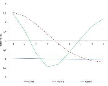
Figure 1: Estimated factors for FA.
-2 -1,5 -1 -0,5 0 0,5 1 1,5 2
1 2 3 4 5 6 7 8 9
F
a
c
to
r
v
a
lu
e
s
Factor 1 Factor 2 Factor 3
The factors are initiated by taking√Ttimes the eigenvectors corresponding to the largest
eigenvalues of theT×Tmatrix∑iN=1yiy′i/N. To get a feeling for what the extracted factors
look like, Figure 1 plots the values of the factors associated with the three largest eigenvalues
for FA. The first factor is almost a straight line, suggesting that this factor is in fact
captur-ing unit-specific fixed effects. The remaincaptur-ing two factors resemble a cubic line with a large
smoothing parameter and a quadratic line. This demonstrates the importance of allowing
for nonlinear effects, casting doubt on existing results based on fixed effects-only unit root
tests. The factors for EMP are almost identical and are therefore not plotted. In fact, the
cor-relation between the second (third) factor of the two variables is 0.99 (0.98). Hence, at least
the common part of FA and EMP seems to be measuring the same thing.
In order to gauge against possible serial correlation in the errors, we implement our
GMM approach assuming MA errors of orderq∈ {1, 2}. If the model is misspecified, this is
and use the BIC1 criterion of Ahn et al. (2013) to pick the most appropriate number, given
that it passes the Hansen–Sargan test at the 5% level.
5.3 Results
Table 3 reports results obtained based on the two-step GMM estimator, GMM2. The results
are very similar for EMP and FA. In particular, the point estimate ofρ0is below unity, but the
unit root null is not rejected even at the liberal 10% level, suggesting that Gibrat’s law is
sup-ported by the data. The null hypothesis of instrument validity/correct model specification
is also not rejected. For EMP the best fitting model according to BIC1 has two factors and
allows for MA(1) errors, while for FA the preferred model includes one factor and MA(2)
errors.
Our results are consistent with previous findings in the banking literature, which
sug-gest the presence of constant returns to scale (see, for example, Robertson et al., 2013). As
discussed by Simon and Bonini (1958) constant returns to scale corroborates Gibrat’s law
because in this case the probability of a given change in firm size (in proportion to current
size) is likely to be the same for all firms in the industry.
6
Conclusion
This paper develops a GMM-based approach that enable unit root testing in panels whereN
is large and Tis finite. The assumption that Tfinite makes our test suitable for both micro
and small-Tmacro panels. The DGP considered is very general and accommodate an
unre-stricted trend function and cross-section dependence in the form of common factors. These
allowances make the new approach one of the most general around. Indeed, as far as we are
aware, this is the only fixed-Tunit root test approach that can be applied in the presence of
cross-section dependence and/or a potentially non-linear trend function. The approach is
also very simple to implement. In particular, since deterministic terms are treated as
addi-tional common factors, which are estimated, there is no need to model the deterministic part.
Our results show that the new GMM-based unit root test statistic is asymptotically invariant
to both the true and fitted deterministic trend function. Hence, unlike existing tests, with
the new test there is no need for any mean and/or variance correction factors that reflect the
fitted deterministic specification. The limiting distribution of the GMMt-statistic is normal
existing tests, with this test there is no discontinuity in the asymptotic distribution at unity.
References
Abadir, K. M., and J. R. Magnus (2005). Matrix Algebra, Econometric Exercises 1. Cambridge
University Press, New York.
Anderson, T. W., and C. Hsiao (1981). Estimation of Dynamic Models with Error
Compo-nents. Journal of American Statistical Association76, 598–606.
Arellano, M., and S. Bond (1991). Tests of Specification for Panel Data: Monte Carlo
Ev-idence and an Application to Employment Equations. Review of Economic Studies58,
277–297.
Bai, J. (2009). Panel Data Models with Interactive Fixed Effects.Econometrica77, 1229–1279.
Bai, J. (2013). Fixed-Effects Dynamic Panel Models, a Factor Analytical Method.
Economet-rica81, 285–314.
Bai, J., and S. Ng (2004). A Panic Attack on Unit Roots and Cointegration. Econometrica72,
1127–1177.
Bai, J., and S. Ng (2010). Panel Unit Root Tests With Cross-Section Dependence: A Further
Investigation. Econometric Theory26, 1088–1114.
Baltagi, B. (2008). Econometric Analysis of Panel Data, Fourth Edition. John Wiley & Sons,
New York.
Blundell, R., and S. Bond (1998). Initial Conditions and Moment Restrictions in Dynamic
Panel Data Models.Journal of Econometrics87, 115–143.
Bond, S., C. Nauges, and F. Windmeijer (2005). Unit Roots: Identification and Testing in
Micro Panels. Unpublished manuscript.
Breitung, J., and H. Pesaran (2008). Unit Roots and Cointegration in Panels. In L. Matyas
and P. Sevestre (ed.),The Econometrics of Panel Data.
Bun, M., and F. Windmeijer (2010). The Weak Instrument Problem of the System GMM
Estimator in Dynamic Panel Data Models.Econometrics Journal13, 95–126.
Bun, M. ,and V. Sarafidis (2013). Dynamic Panel Data Models. In B. H. Baltagi (ed.),The
Caves, R. E. (1998). Industrial Organization and New Findings on the Turnover and
Mobil-ity of Firms.Journal of Economic Literature36, 1947-1982.
Chesher, A. (1979). Testing the Law of Proportionate Effect. Journal of Industrial Economics
27, 403–411.
De Blander, R., and G. Dhaene (2013). Unit Root Tests for Panel Data with AR(1) Errors and
SmallT.Econometrics Journal15, 101–124.
De Silva, S., K. Hadri and A. R. Tremayne (2009). Panel Unit Root Tests in the Presence of
Cross-Sectional Dependence: Finite Sample Performance and an Application.
Econo-metrics Journal12, 340–366.
De Wachter, S., R. Harris, and E. Tzavalis (2007). Panel Data Unit Roots Tests: The Role of
Serial Correlation and the Time Dimension. Journal of Statistical Planning and Inference
137, 230–244.
Hadri, K., and R. Larsson (2005). Testing for Stationarity in Heterogeneous Panel Data
where the Time Dimension is Finite.Econometrics Journal8, 55–69.
Han, C., and P. C. B. Phillips (2010). GMM Estimation for Dynamic Panels with Fixed
Effects and Strong Instruments at Unity.Econometric Theory26, 119–151.
Harris, R., and E. Tzavalis (1999). Inference for Unit Roots in Dynamic Panels where the
Time Dimension is Fixed.Journal of Econometrics91, 201–226.
Harris, R., and E. Tzavalis (2004). Testing for Unit Roots in Dynamic Panels in the Presence
of a Deterministic Trend: Re-examining the Unit Root Hypothesis for Real Stock Prices
and Dividends.Econometric Reviews23, 149–166.
Hlouskova, J., and M. Wagner (2006). The Performance of Panel Unit Root and Stationarity
Tests: Results from a Large Scale Simulation. Econometric Reviews25, 85–116.
Im, K. S., M. H. Pesaran and Y. Shin (2003). Testing for Unit Roots in Heterogeneous Panels.
Journal of Econometrics115, 53–74.
Kruiniger, H. (2007). An Efficient Linear GMM Estimator for the Covariance Stationary
Kruiniger, H. (2009). GMM Estimation and Inference in Dynamic Panel Data Models with
Persistent Data. Econometric Theory25, 1348–1391.
Kruiniger, H. (2013). Quasi ML Estimation of the Panel AR(1) Model with Arbitrary Initial
Conditions. Journal of Econometrics173, 175–188.
Madsen, E. (2010). Unit Root Inference in Panel Data Models where the Time-Series
Dimen-sion is Fixed: A Comparison of Different Tests.Econometrics Journal13, 63–94.
Moon, H. R., and B. Perron (2004). Testing for Unit Root in Panels with Dynamic Factors.
Journal of Econometrics122, 81–126.
Levin, A., C. Lin, and C.-J. Chu (2002). Unit Root Tests in Panel Data: Asymptotic and
Finite-sample Properties.Journal of Econometrics108, 1–24.
Pesaran, M. H. (2007). A Simple Panel Unit Root Test in the Presence of Cross Section
Dependence. Journal of Applied Econometrics22, 265–312.
Phillips, P. C. B., and D. Sul (2003). Dynamic Panel Estimation and Homogeneity Testing
Under Cross Section Dependence.Econometrics Journal6, 217–259.
Roberston, D., and V. Sarafidis (2013). IV Estimation of Panels with Factor Residuals.
Un-published manuscript.
Robertson, R., V. Sarafidis and T. Yamagata (2013). Estimation of Correlated Random
Co-efficient Models for Short Panels with a Multi-Factor Error Structure. Unpublished
manuscript.
Sarafidis, V., and T. Wansbeek (2012). Cross-Sectional Dependence in Panel Data Analysis.
Econometric Reviews31, 483–531.
Simon, H. A., and C. P. Bonini (1958). The Size Distribution of Business Firms. American
Economic Review58, 607–617.
Steindl, J. (1965).Random Processes and the Growth of Firms: a Study of the Pareto Law. Hafner
Publishing, New York.
Westerlund, J., and J. Breitung (2013). Lessons from a Decade of IPS and LLC.Econometric
Appendix: Proofs
This Appendix makes heavy use of the results of Abadir and Magnus (2005). Here now we
state some of the most frequently used results. ThroughoutA,B,CandDare going to
de-note generic matrices of dimensionm×p,n×q,k×randl×s, respectively. We also denote
byKmp themp×mpcommutation matrix of zeroes and ones suchKmpvecA= vecA′. IfA
ism×m(square), then we denote byDmthem2×m(m+1)/2 duplication matrix of zeroes
and ones such thatDmvechA=vecA. The following results are going to be used frequently
in the sequel:
• vec(ABC) = (C′⊗A)vecB;
• vec(A⊗B) = (Ip⊗Kqm⊗In)(vecA⊗vecB);
• (A⊗B)(C⊗D) = (AC⊗BD), ifACandBDare defined;
• Kmn(A⊗B) = (B⊗A)Kqp.
We also define the matrix derivative operator Dx, which is such that if the matrix
func-tionR(x)ism×p andx isn×q, then DxR(x) = ∂vecR(x)/∂(vecx)′ ismp×nq. Hence,
denoting by d the matrix differential, then we have d vecR(x) =A(x)d vecx, or DxR(x) =
d vecR(x)/d vecx. Also, if R(x) is a m×m and symmetric, then we define DxR(x) =
∂vecR(x)/∂(vechx)′. Dq
xR(x)means DqxR(x) = ∂qvecR(x)/[∂(vecx)′]. Some important
rules for differentials:
• d[R(x)G(x)] = [dR(x)]G(x) +R(x)dG(x);
• d[R(x)⊗G(x)] = [dR(x)]⊗G(x) +R(x)⊗dG(x).
Proof of Theorem 1.
Note that vec(F0Σ
λF′) = (F⊗F0)vecΣλ, where vecΣλ= DrvechΣλ =Drθ2. It follows that
vec[Γ(ρ)F0ΣλF′IT] = [IT ⊗Γ(ρ)]vec(F0ΣλF′) = [IT⊗Γ(ρ)](F⊗F0)Drθ2, whereΓ = Γ(ρ)
has been written as a function ofρ. Making use of this result, it is clear that
S(IT⊗Γ(ρ)F0ΣλF′)e = (e′⊗S)vec[IT⊗Γ(ρ)F0ΣλF′]
= (e′⊗S)(IT⊗KT2⊗IT)[vecIT⊗vec(Γ(ρ)F0ΣλF′)]
Moreover, since vecIT has just one column,
[vecIT⊗(IT⊗Γ(ρ))(F⊗F0)Drθ2] = [vecIT⊗(IT⊗Γ(ρ))(F⊗F0)Dr](1⊗θ2)
= [vecIT⊗(IT⊗Γ(ρ))(F⊗F0)Dr]θ2.
Hence,
W1/2S(IT⊗Γ(ρ)F0ΣλF′)e=R(ρ)θ2,
whereR(ρ) = W1/2C1U(ρ),C1 = (e′⊗S)(IT ⊗KT2⊗IT)isT(T+1)/2×T4andU(ρ) =
[vecIT⊗(IT⊗Γ(ρ))(F⊗F0)Dr]isT4×r(r+1)/2. g(θ)can therefore be rewritten as
g(θ) = W1/2(mˆ −ρmˆ0−S[IT⊗ΓF0ΣλF′]e)
= W1/2(mˆ −ρmˆ0)−W1/2S[IT⊗ΓF0ΣλF′]e
= W1/2(mˆ −ρmˆ0)−R(ρ)θ2, (A1)
suggesting that
d vecg(θ) =dg(θ) =−R(ρ)dθ2, (A2)
where the differential is taken with respect to θ2 (treating ρ as fixed). The corresponding
derivative is given by
Dθ2g(θ) =−R(ρ), (A3)
which in turn implies
Dθ2Q(θ) =2g(θ)
′D
θ2g(θ) =−2g(θ)
′R(ρ). (A4)
The relevant first-order condition is therefore given by
[W1/2(mˆ −ρmˆ0)−R(ρ)θ2]′R(ρ) =01×r(r+1)/2, (A5)
or
R(ρ)′W1/2(mˆ −ρmˆ0) =R(ρ)′R(ρ)θˆ2.
The r(r+1)/2×r(r+1)/2 matrix R(ρ)′R(ρ) is nonsingular. Hence, defining ˆz
T(ρ) =
W1/2(mˆ −ρmˆ0), we have ˆ
θ2= [R(ρ)′R(ρ)]−1R(ρ)′ˆzT(ρ). (A6)
The concentrated version ofg(θ)is
gC(ρ) = g(ρ, ˆθ2(ρ)) =W1/2(mˆ −ρmˆ0)−R(ρ)θˆ2(ρ) (A7)