Munich Personal RePEc Archive
Modeling Covariance Breakdowns in
Multivariate GARCH
Jin, Xin and Maheu, John M
Shanghai University of Finance and Economics, DeGroote School of
Business, McMaster University
10 April 2014
Online at
https://mpra.ub.uni-muenchen.de/55243/
Modeling Covariance Breakdowns in Multivariate
GARCH
∗
Xin Jin
†John M. Maheu
‡March 2014
Abstract
This paper proposes a flexible way of modeling dynamic heterogeneous covariance breakdowns in multivariate GARCH (MGARCH) models. During periods of normal market activity, volatility dynamics are governed by an MGARCH specification. A covariance breakdown is any significant temporary deviation of the conditional covari-ance matrix from its implied MGARCH dynamics. This is captured through a flexible stochastic component that allows for changes in the conditional variances, covariances and implied correlation coefficients. Different breakdown periods will have different impacts on the conditional covariance matrix and are estimated from the data. We propose an efficient Bayesian posterior sampling procedure for the estimation and show how to compute the marginal likelihood of the model. When applying the model to daily stock market and bond market data, we identify a number of different covariance breakdowns. Modeling covariance breakdowns leads to a significant improvement in the marginal likelihood and gains in portfolio choice.
JEL: C32, C51, C58
key words: correlation breakdown, marginal likelihood, particle filter, Markov chain, generalized variance
∗We thank Jeroen Rombouts for comments on an earlier version of this paper. We thank Jia Liu and
conference participants at CFE’13 for helpful comments. Maheu is grateful to the SSHRC for financial support.
†Shanghai University of Finance and Economics, [email protected]
‡DeGroote School of Business, McMaster University, 1280 Main Street West, Hamilton, ON, Canada,
1
Introduction
This paper proposes a flexible way of modeling dynamic heterogeneous covariance break-downs in multivariate GARCH (MGARCH) models. During periods of normal market activ-ity, volatility dynamics are governed by an MGARCH specification. A covariance breakdown is any significant temporary deviation of the conditional covariance matrix from its implied MGARCH dynamics. A covariance breakdown is captured through a flexible stochastic component that allows for changes in the conditional variances, covariances and implied correlation coefficients.
It is widely acknowledged that markets face periods that are characterized by abnormal behavior. Several approaches have been used to capture changes in the dynamics of con-ditional second moments including dynamic copulas (Kenourgios et al. 2011, Christoffersen et al. 2012), and the factor spline GARCH model of Rangel & Engle (2012).1 Dufays (2013)
uses an infinite-state hidden Markov model to allow for parameter change in Engle’s (2002) dynamic conditional correlation model. The path dependence that the latent state variable causes in the GARCH recursions is removed following the ideas in Klaassen (2002).2 Haas
& Mittnik (2008) and Chen (2009) extend the univariate MS-GARCH model in Haas et al. (2004) to a multivariate setting. Their model assumes there are K parallel MGARCH models running at the same time, where K is the number of states. Silvennoinen & Tersvirta (2009) apply the smooth transition modeling approach to conditional correlations. Other regime-switching approaches include Ang & Bekaert (2004), Guidolin & Timmermann (2006) and Pelletier (2006).
In contrast to the literature, which has tended to focus on correlation breakdowns, we investigate breakdowns in each component of the conditional covariance matrix. This has several advantages. First, we can see how conditional correlations are affected through vari-ances and covarivari-ances. Second, by modeling the full covariance matrix we avoid issues of misspecification by focusing only on correlations (Forbes & Rigobon 2002) and neglecting heteroskedasticity. In our model a covariance breakdown does not necessarily imply a corre-lation breakdown or contagion effect. It depends on the relative changes in the conditional covariance and conditional variances. Empirically we identify both covariance breakdowns which lead to correlation changes and breakdowns which have little impact on correlations. To our knowledge this is the first paper to explicitly model the dynamics of conditional covariance breakdowns and estimate their impacts. In our approach a covariance breakdown is any sustained deviation of the conditional second moments from the covariance matrix implied by the MGARCH specification. Each breakdown period is different and estimated from the data. Covariance breakdowns as well as normal periods are assumed to follow a first-order Markov chain. Each breakdown is characterized by a random matrix drawn from an inverse-Wishart distribution that scales (multiplies) the MGARCH covariance matrix.3
1
It is important to account for changes in GARCH dynamics. For instance, in the univariate setting, neglected parameter changes in volatility dynamics can bias GARCH parameter estimates toward higher persistence and lead to poor forecasts of volatility (Lamoureux & Lestrapes 1990, Hillebrand 2005).
2
Another approach to dealing with path dependence directly is the particle MCMC approach of Bauwens et al. (2014).
3To be precise, a positive definite matrix drawn from an inverse-Wishart density is sandwiched between
This approach is very flexible while retaining a positive definite matrix. Since covariance breakdowns are finite, they eventually end and we return to a model in which the MGARCH dynamics solely determine conditional second moments.
Our model can be considered as an extension to Markov switching models. Bayesian inference for Markov regime-switching models is usually carried out based on the forward-backward algorithm of Chib (1996). Our approach is different than the conventional regime-switching specification in which model parameters governing a time period are selected from a fixed parameter set. A covariance breakdown is captured by introducing an exogenous stochastic multiplicative component to the volatility matrix itself. This requires a new posterior sampling approach for the states. We construct an efficient sampling scheme to sample the unobserved state variables as well as other fixed parameters.
Whether covariance breakdowns are supported by the data can be formally assessed in the context of Bayesian model comparison by making use of the marginal likelihood. We show how to compute the marginal likelihood and design a particle filter for the task.
The model is applied to daily excess returns on the S&P 500 index and short-term and long-term bonds over a twenty-five year period. Including fat-tailed return innovations in the model is important in distinguishing between outliers and sustained covariance breakdowns. We compare our model to an MGARCH model with Student-t innovations but with no breakdowns. Bayes factors strongly support the inclusion of covariance breakdowns. The volatility dynamics during breakdown periods are very different for the two models as well as breakdowns being different over time. For example, in the recent financial crisis we identify an initial breakdown which leads to an overall increase in variability. This features large increases in conditional variances and drops in covariances between the stock and bond market. However, the conditional correlations do not show a dramatic change. Following this episode is another breakdown which is characterized as a reduction in overall variability. Estimates indicate that covariance breakdowns occur 34% of the time and their expected duration is 1-2 months. The impact of a typical covariance breakdown is expected to increase variability. In addition to improving the fit of the data, modeling covariance breakdowns provides improved portfolio choice.
The rest of the paper is organized as follows. In Section 2, we introduce the breakdown model and discuss its properties. Section 3 constructs a sampling procedure for the posterior inference of the model. Section 4 provides simulation study for illustration. Section 5 shows how to compute the marginal likelihood of our model. In Section 6, we apply the model to study the volatility dynamics among the stock market and the bond market and Section 7 concludes. The Appendix contains details on posterior sampling and computation of the marginal likelihood.
2
Multivariate GARCH with Covariance Breakdowns
Consider a k-dimensional vector time series yt, t = 1,2,3, . . .. Let Ft−1 be the sigma field
generated by the past values of yt until timet−1. Consider the following model
yt=µ+Ht1/2Λ
1/2
where µ =E(yt|Ft−1) is the constant conditional mean4 vector and zt ∼N ID(0, I).5 Ht1/2
denotes the Cholesky factor of thek×kpositive definite matrixHt, which is assumed to follow
any of the popular specifications for the MGARCH model. Popular examples of MGARCH models include, among others, the vector-diagonal GARCH (VDGARCH) by Ding & Engle (2001) and the dynamic conditional correlation (DCC) by Engle (2002). See Bauwens et al. (2006) for a review.
The latent discrete state variablest∈ {1,2}is assumed to direct the dynamics of Λt and
follows a two-state first-order Markov chain with transition matrix
P =
π1 1−π1
1−π2 π2
, (2)
which divides the sample path into periods ofnormal states (st= 1) and periods ofcovariance
breakdown states (st = 2). We impose the constraint π1 > π2 to identify normal periods as
being more frequent than covariance breakdowns. If s1:t={s1, ..., st}, then Λt is determined as follows
Λt|s1:t=
I if st= 1
Λt−1 if st= 2, st−1 = 2
∼G0 if st= 2, st−1 = 1
(3)
G0 can be any distribution over symmetric positive definite matrices. In this paper, we
use an inverse-Wishart distribution W−1(ν, Q
0), with first moment Q0/(ν −k−1), where
ν > k−1 is the scalar degree of freedom and Q0 is the k ×k symmetric positive definite
scale matrix. The choice of inverse-Wishart distribution aids in posterior sampling and will be discussed in more detail in Section 3.
Some key features of the model are as follows. First, there remains an MGARCH structure in the volatility dynamics that is represented byHt. However, with the addition of Λt in the
structure, Ht is no longer the conditional covariance matrix ofyt as is the case with the
con-ventional MGARCH models since Var(yt|Λt,Ft−1) = Ht1/2Λt(Ht1/2) ′
. Second, st determines
the underlying state of the volatility dynamics ofyt. st= 1, Λt=I denotes the normal state
in which volatility dynamics are solely driven by Ht from the MGARCH structure, where
Var(yt|Λt = I,Ft−1) = Ht. A change from the underlying MGARCH covariance dynamics
begins when the state switches fromst−1 = 1 tost= 2, which signals the beginning of a
break-down period. In this case, Λt is a new draw from G0 and Var(yt|Λt,Ft−1) = Ht1/2Λt(Ht1/2) ′
in general will not be equal to Ht. As a result, the volatility starts to deviate from Ht. If
st+1 = 2 the breakdown period continues and Λt+1 = Λt, while the MGARCH component
changes to Ht+1. In this way we isolate the tendency of a covariance breakdown period to
display a constant impact on Ht such as driving up conditional correlations or depressing
conditional variances. The breakdown continues until the state switches back to 1, and we are back in the normal state, where the volatility once again coincides with Ht.
In each breakdown period Λt is constant and has the same impact on Ht. On the other
hand, different breakdown periods will have their unique break patterns, e.g. increased vari-ability or decreased varivari-ability, etc., as each breakdown period is characterized by a unique
4A time-varying conditional mean can also be used.
5Other distributions such as a Student-t could be used forztas long as a normal decomposition can be
Λt drawn from G0. Thus even though st is a two-state Markov chain and the volatility
dynamics can only alternate between normal periods and breakdown periods, the break-down periods are “heterogeneous” and there could be infinitely many “types” of covariance breakdowns. Hence this modeling structure distinguishes itself from a standard two-state regime-switching approach which moves between two fixed parameter vectors. The model is also different from the (infinite dimension) structural break model. In structural break models, past states (periods) cannot recur. Whereas in our model, the volatility dynamics can always revert to the normal statest= 1.
The functional form for covariance breakdowns Ht1/2Λt(Ht1/2) ′
is convenient in that it remains positive definite and a well defined conditional covariance matrix. In general, Λt can
inflate or shrink the elements ofHt. One overall measure of variability is the determinant of
the covariance matrix, also called thegeneralized variance by Muirhead (1982). The relative change in the generalized variance is |Ht1/2Λt(Ht1/2)
′
|/|Ht| = |Λt|. Λt can either increase or
decrease the generalized variance depending on whether its own determinant is greater or less than 1.
In addition to the direct effect on the covariance matrix, Λt also has an indirect effect
on future volatility through the feedback from the current volatility matrix to future Ht.
Any of the usual MGARCH specifications for Ht+1 depends on the cross-products of yt, the
distribution of which is a function ofHt1/2Λt(Ht1/2) ′
. If Λt 6=I, it will affectHt+1 through the
realized value of yt. As a result, during a breakdown period, the instantaneous impact of Λt
on the conditional second moments is compounded over time with the help of the feedback channel. An important implication is that the model may accommodate breakdown periods that feature local nonstationarity.
This model is flexible in allowing for various changes in the conditional covariance matrix. Consider the following example. Let
H =
2 1.5
1.5 3
.
We draw several random Λ fromG0 =W−1(7,4I) and compute V =H1/2Λ(H1/2)
′
.6 Table 1
records the changes in the elements as well as the implied correlation coefficient ofV relative to those ofH for different Λ. Various scenarios can occur. For example, we have cases where the variances, the covariance, and the correlation coefficient all increase (or decrease), and we have cases where the variances and the covariance increase (or decrease) in a way that the correlation coefficient remains relatively constant. There can be times when the variances go up but the covariance goes down and even becomes negative. Other times the two variances can move in opposite directions. This particular form for covariance breakdowns allows for a wide variety of effects on the conditional second moments that can be estimated from the data.
In another example, assume the following VDGARCH specification
Ht = CC′+aa′⊙yt−1yt′−1+bb′⊙Ht−1 (4)
where C is a k×k lower triangular matrix, a and b are k ×1, ⊙ denotes the element-by-element matrix product (Hadamard product). Let G0 be the same distribution as above.
6
E(Λ) = 4I
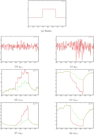
Three episodes of the simulated data are shown in Figure 1 to 3 displaying the data, states and elements of the total conditional covariance matrix Vt = (vij,t) = Ht1/2Λt(Ht1/2)
′
) as well as the corresponding values from Ht = (hij,t). All three episodes have one breakdown
period, but the break patterns are different from one another. In the first episode, the breakdown period features a sharp surge in both conditional variances and the conditional covariance. The correlation coefficient also jumps up from below 0.3 to around 0.9. The associated Λ = (λij) 7 for this breakdown period is λ11 = 6.62, λ21 = 1.86, λ22 = 1.46. Its
determinant is |Λ| = 6.20, indicating an increase in the overall variability. In the second episode, the breakdown period causes both variances to increase, while inducing a strong drop in the correlation between y1,t and y2,t. Here λ11 = 1.35, λ21 = −0.98, λ22 = 1.47,
and |Λ|= 1.02, which means no change in the overall variability. For the third episode, the two variances move in opposite directions during the breakdown period and the correlation switches signs as the breakdown period starts and becomes very negative until the normal period is restored, by which time the correlation becomes positive again.
In summary, this modeling approach is flexible enough to accommodate different abrupt changes that lead to significant deviations from the underlying MGARCH structure.
3
Model Inference
We apply a Bayesian approach to model estimation where Markov chain Monte Carlo (MCMC) methods are used for posterior inference. The unknown parameters of the model consist ofπ1, π2,Θ, µ, where Θ denotes the set of parameters in the GARCH specification that
governs Ht. For example, if the VDGARCH specification in (4) is used, then Θ ={C, a, b}.
We refer to this model with covariance breakdowns as VDGARCH-B. The parameter space is augmented with st and Λt, both of which are jointly estimated with the fixed parameters.
The stochastic nature of Λt makes the posterior sampling of states st more complicated
than a standard Markov switching model in which state-dependent parameters are fixed over the whole sample. Given the observed data of sample size T, letS ={st}Tt=1, Y ={yt}Tt=1,
Λ={Λt}Tt=1, a hybrid MCMC algorithm can be designed to sample from the joint posterior
distribution. To sample from p(π1, π2,Θ, µ,S,Λ|Y), we propose an efficient sampler that
iteratively samples through the conditional posterior distribution of each block:
1. p(S|Θ, π1, π2, µ,Y)
2. p(π1, π2|S),
3. p(Θ|S, µ,Y) 4. p(Λ|S,Θ, µ,Y) 5. p(µ|Λ,Θ,Y).
Taking a draw from all of the conditional distributions constitutes one sweep of the sampler. After dropping an initial set of draws as burn-in we collectM draws{π1(i), π2(i),Θ(i), µ(i),S(i),Λ(i)}M
i=1
for posterior inference. Simulation consistent estimates of posterior moments can be obtained as sample averages of the draws. For instance, the posterior mean of π1 can be estimated as
M−1PM i=1π
(i)
1 . Next we discuss each block in more detail.
7The subscripttof Λ
3.1
Sampling S
Conditional on Ht and µ, apply the transformation
˜
yt=Ht−1/2(yt−µ), (5)
so that
˜
yt|Λt∼N(0,Λt). (6)
Let ˜Y ={y˜t}Tt=1 be the transformed data. Sampling from p(S|Θ, π1, π2, µ,Y) is equivalent
to sampling from p(S|π1, π2,Y˜).
We sequentially sample from the two-point discrete distributions p(st|S−t, π1, π2,Y˜) for
t= 1, . . . , T, whereS−t =S\st. It requires calculatingP r(st= 1|S−t, π1, π2,Y˜) andP r(st=
2|S−t, π1, π2,Y˜) for eacht. Lett1, t2 be integers such thatT ≥t1 ≥1,T ≥t2 ≥1. There are
several cases depending on the values ofS−t. Suppress π1, π2 in the conditioning set for the
moment and writep(˜yt|Λ) =N(˜yt|0,Λ),p(Λ) =W−1(Λ|ν, Q0), whereN(.|., .) andW−1(.|., .)
are the density functions of the normal distribution and the inverse-Wishart distribution, respectively. The cases are:
• st−t1−1 = 1, st−t1 =· · ·=st−1 = 2, st+1 =· · ·=st+t2 = 2, st+t2+1 = 1
P r(st = 1|S−t,Y˜) ∝
"Z Y−1
j=−t1
p(˜yt+j|Λ)
!
p(Λ)dΛ
#
p(˜yt|st = 1)
"Z Yt2
j=1
p(˜yt+j|Λ)
!
p(Λ)dΛ
#
×P r(st= 1|st−1 = 2)P r(st+1 = 2|st= 1)
P r(st = 2|S−t,Y˜) ∝
"Z Yt2
j=−t1
p(˜yt+j|Λ)
!
p(Λ)dΛ
#
P r(st= 2|st−1 = 2)P r(st+1 = 2|st= 2).
• st−1 = 1, st+1 =· · ·=st+t2 = 2, st+t2+1 = 1
P r(st = 1|S−t,Y˜) ∝ p(˜yt|st = 1)
"Z Yt2
j=1
p(˜yt+j|Λ)
!
p(Λ)dΛ
#
×P r(st= 1|st−1 = 1)P r(st+1 = 2|st= 1)
P r(st = 2|S−t,Y˜) ∝
"Z Yt2
j=0
p(˜yt+j|Λ)
!
p(Λ)dΛ
#
P r(st = 2|st−1 = 1)P r(st+1 = 2|st = 2).
• st−t1−1 = 1, st−t1 = 2 =· · ·=st−1 = 2, st+1 = 1
P r(st = 1|S−t,Y˜) ∝
"Z Y−1
j=−t1
p(˜yt+j|Λ)
!
p(Λ)dΛ
#
p(˜yt|st = 1)
×P r(st= 1|st−1 = 2)P r(st+1 = 1|st= 1)
P r(st = 2|S−t,Y˜) ∝
"Z Y0
j=−t1
p(˜yt+j|Λ)
!
p(Λ)dΛ
#
• st−1 = 1, st+1 = 1
P r(st = 1|S−t,Y˜) ∝ p(˜yt|st = 1)P r(st = 1|st−1 = 1)P r(st+1 = 1|st= 1)
P r(st = 2|S−t,Y˜) ∝
Z
p(˜yt|Λ)p(Λ)dΛ
P r(st = 2|st−1 = 1)P r(st+1 = 1|st= 2).
In all cases,8 we need to compute the integral R Qt4
t=t3p(˜yt|Λ)
p(Λ)dΛ for some t3 and t4
with T ≥t4 ≥t3 ≥0. We show in the Appendix that
Z Yt4
t=t3
p(˜yt|Λ)
!
p(Λ)dΛ = 2
nk
2 (2π)−
nk
2 |Q0|
ν
2 Qk j=1Γ(
n+ν+1−j
2 )
|Q|n+2ν Qk j=1Γ(
ν+1−j
2 )
, (7)
where Q=Pt4t=t3y˜ty˜′t+Q0, andn =t4−t3+ 1.
3.2
Sampling
π
1,
π
2The conditional posterior distributions are:
p(π1|S)∝p(S|π1)p(π1)∝p(π1)π1n1(1−π1)n2 (8)
and
p(π2|S)∝p(S|π2)p(π2)∝p(π2)π2n3(1−π2)n4 (9)
where
n1 = #{t∈ {1, . . . , T −1}|st= 1, st+1 = 1}, n2 = #{t ∈ {1, . . . , T −1}|st = 1, st+1 = 2}
n3 = #{t∈ {1, . . . , T −1}|st= 2, st+1 = 2}, n4 = #{t ∈ {1, . . . , T −1}|st = 2, st+1 = 1},
and # denotes the number of elements in a set. p(π1) and p(π2) are prior distributions.
For the choice of priors, let π1 ∼ Beta(απ1, βπ1) and π2 ∼ Beta(απ2, βπ2), where Beta(., .)
denotes the beta distribution. Then we have the Gibbs sampling step
π1|S∼Beta(¯απ1,β¯π1) and π2|S∼Beta(¯απ2,β¯π2) (10)
where ¯απ1 = απ1 +n1, ¯βπ1 = βπ1 +n2, ¯απ2 = απ2 +n3 and ¯βπ2 = βπ2 +n4. If we impose
the restriction π1 > π2, we can jointly sample π1 and π2 using a Metropolis-Hastings (M-H)
step with independent joint proposal of π′
1, π2′ from (10). The proposal is accepted with
probability α((π1, π2),(π1′, π2′)|S) = Iπ′ 1>π2′.
8
s1 and sT are sampled in similar fashion as other cases by excluding P r(s1 = 1,2|s0 = 1,2) and
3.3
Sampling
Θ
The likelihood function p(Y|Θ, µ,S) can be computed by integrating out Λ as
p(Y|Θ, µ,S) =
Z
p(Y|Θ, µ,Λ)p(Λ|S)dΛ
=
Z YT
t=1
p(yt|µ, Ht,Λt)
!
p(Λ|S)dΛ
=
Z YT
t=1
(2π)−k2|H 1 2 t Λt(H
1 2 t )
′
|−12 exp
−1
2(yt−µ)
′(H12 t Λt(H
1 2 t )
′
)−1(yt−µ)
!
p(Λ|S)dΛ
=
" T Y
t=1
|Ht|− 1 2
# Z YT
t=1
(2π)−k2|Λ t|−
1 2 exp
−1
2(H
−12
t (yt−µ)) ′
Λ−t1(H−12
t (yt−µ))
!
p(Λ|S)dΛ
=
" T Y
t=1
|Ht|− 1 2
# Z YT
t=1
(2π)−k2|Λt|−12 exp
−1
2y˜
′ tΛ−t1y˜t
!
p(Λ|S)dΛ
=
" T Y
t=1
|Ht|− 1 2
#
p( ˜Y|S) (11)
The last line in (11) requires the computation of p( ˜Y|S) which depends on the number of breakdown periods in the sample. Suppose, given S, there are B ≥ 0 breakdown period(s) over the whole sample denoted as BP1,BP2, . . . ,BPB. Each BPq starts at date tq,s and
ends at datetq,e ≥tq,s, with durationNq=tq,e−tq,s+ 1. IfBPc denotes the union of all the
normal periods then BPc,BP1,BP2, . . . ,BPB form a partition of {1,2, . . . , T}.
Now
p( ˜Y|S) = Y
t∈BPc
N(˜yt|0, I) B
Y
q=1
Z
Y
t∈BPq
p(˜yt|Λ)
p(Λ)dΛ
= Y
t∈BPc
(2π)−k2 exp(−1
2y˜
′
ty˜t)
YB
q=1
2Nq k2 (2π)−
Nq k
2 |Q0|
ν
2 Qk j=1Γ(
Nq+ν+1−j
2 )
|Qq|
Nb+ν
2 Qk j=1Γ(
ν+1−j
2 )
(12)
where Qq=Pt∈BPqy˜ty˜t′+Q0. The conditional posterior distribution is:
p(Θ|S, µ,Y) ∝ p(Y|Θ, µ,S)p(Θ)∝
" T Y
t=1
|Ht|− 1 2
#
p( ˜Y|S)p(Θ).
(13)
3.4
Sampling Λ
Given S, when st = 1, Λt = I. During a breakdown period, Λt 6=I but remains constant.
The number of unique non-identity Λt is equal to the number of breakdown periods B. Let
˜
Λq be the unique value of Λt realized in BPq. Then the conditional posterior is
˜
Λq ∼W−1(νq, Qq), (14)
where νq =ν+Nq and Qq =Pt∈BPqy˜ty˜t′ +Q0.
3.5
Sampling
µ
Given Λ, Θ andµ, the likelihood function is
p(Y|Λ,Θ, µ) =
T
Y
t=1
N(yt|µ, H 1 2 t Λt(H
1 2 t )
′
), (15)
and the conditional posterior density is
p(µ|Λ,Θ,Y) ∝ p(µ)p(Y|Λ,Θ, µ). (16)
Given prior distributionp(µ) an M-H step is used to sample from the posterior distribution. We specify an independent Gaussian prior.
This covers the steps for posterior simulation of the model. We now consider two impor-tant extensions to the basic covariance breakdown model.
3.6
Student-t innovations
A multivariate Student-t distribution can be used in place of the Gaussian assumption to account for fat tails. In the case of a VDGARCH specification, we refer to the fat-tailed version of the breakdown model as VDGARCH-t-B. Only minor adjustments on the original samplers are needed as a Student-t random variable can be written as a ratio of a Gaussian variable and the square root of a Gamma random variable.9 More specifically, if y
t follows a
Student-t distribution with meanµ, scale matrixHt1/2Λt(Ht1/2) ′
and degree of freedomd >2, oryt∼t(µ, Ht1/2Λt(Ht1/2)
′
, d), then it can be written as
yt = µ+ut−1/2(yt∗−µ), (17)
where
y∗t ∼ N(µ, Ht1/2Λt(Ht1/2) ′
) (18)
ut ∼ G(d/2, d/2). (19)
To facilitate posterior sampling, data augmentation is implemented again by treating
U = {ut}Tt=1 as unknown parameters. In this case, the full set of conditional posterior
9Denote a Gamma distribution asG(a, b) which has meana/b, and denote the associated density function
distributions consists of two more components: p(U|Θ,Λ, µ, d,Y) and p(d|U). To sample
U, let Vt=Ht1/2Λt(Ht1/2) ′
and note
p(ut|yt,Θ,Λ, µ, d) ∝ p(ut)p(yt|ut,Θ,Λ, µ)
∝ G(ut|d/2, d/2)N(yt|µ, u−t1Vt)
= ud/t 2−1e−dut/2(2π)−k/2|u−1
t Vt|−1/2e− 1
2(yt−µ)′(u−1t Vt)−1(yt−µ)
∝ u
k+d
2 −1 t e−
1
2ut(d+(yt−µ)′V −1
t (yt−µ))
∝ G ut
k+d
2 ,
1
2(d+ (yt−µ)
′V−1
t (yt−µ))
!
. (20)
To sample d, let the prior of d follows a truncated exponential distribution with density function p(d) ∝ Exp(d|λ0)Id>2, where Exp(d|λ0) = λ0e−λ0d is the density function of an
exponential distribution with mean equal to λ01 . Then
p(d|U) ∝ p(d)p(U|d)
∝ Exp(d|λ0)Id>2
T
Y
t=1
(d2)d/2
Γ(d
2)
ud/t 2−1e−dut/2
∝ λ0e−λ0dId>2
(d2)d/2
Γ(d2)
!T
exp −d
2
T
X
t=1
(ut−log (ut))
!
. (21)
The posterior can be sampled using an M-H step.
Givenµandut, letyt∗ = (yt−µ)ut1/2+µand writeY∗ ={yt∗}Tt=1. The sampling procedure
for the Student-t model consists of sequential draws from the following conditional posterior distributions10:
1. p(S|Θ, π1, π2, µ,Y∗),
2. p(π1, π2|S),
3. p(Θ|S, µ,Y∗),
4. p(Λ|S,Θ, µ,Y∗),
5. p(µ|Λ,Θ,Y∗),
6. p(U|Θ,Λ, µ, d,Y), 7. p(d|U).
Steps 1-5 are a repeat of the sampling steps in the Gaussian model but conditional on Y∗
and require no additional coding.
3.7
Learning about Covariance Breakdowns
So far we have assumed G0 = W−1(ν, Q0) with known parameters ν and Q0. We can also
introduce a hierarchy and place prior distributions on ν and Q0 . By incorporating both
10Note that the conditional posterior distributions ofS, π
1, π2,Θ,Λ, µare each conditioned on the
parameters into the posterior sampling scheme, we can learn about the typical effect of Λt.
As shown in Section 8.2, sampling of ν and Q0 can be included in the posterior sampling
algorithm as an M-H step and a Gibbs step, respectively.
4
Simulation Study
To analyze the performance of the proposed estimation algorithm, we conduct a simulation
study in a 2×2 dimension. We simulate 5000 observations from a VDGARCH-B model.
The parameters are
C =
0.04 0
0.01 0.03
, a= (0.12,0.1)′, b = (0.97,0.98)′, π1 = 0.99, π2 = 0.98, µ= 0.
A Gaussian distribution is assumed for the innovations and learning aboutG0 is ignored and
instead specified asG0 =W−1(7,4I) so thatE[Λt] = I. The prior distributions are as follows:
π1 ∼ Beta(3,0.1), π2 ∼ Beta(2,0.1); Cii ∼ T N+(0,100) for i = 1,2, C21 ∼ N(0,100);
a1 ∼ T N+(0,100), a2 ∼ N(0,100); b1 ∼ T N+(0,100), b2 ∼ N(0,100). T N+(.) denotes the
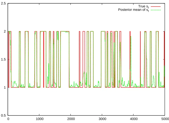
truncated Gaussian distribution on the positive real line. In the posterior sampling, the first 10000 MCMC draws are discarded as burn-in and the next 10000 draws are used for inference.
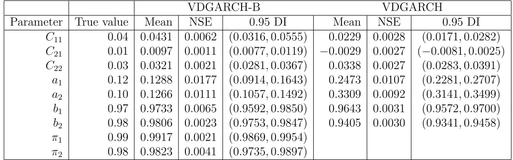
Parameter estimates are reported in Table 2. All parameter values are accurately recov-ered. Figure 4 displays the posterior mean of st, compared with the true states over time
and shows that the model identifies the breakdown periods and normal periods well.
For comparison, we also estimate a plain VDGARCH model that does not allow for covariance breakdowns with the same data. This model can be seen as a special case or restricted version of our model with π1 = 1 and s1 = 1. The parameter estimates are
reported in Table 2.11 The results are very different from the true values, which is not
surprising due to misspecification. For example, the posterior means of a1 and a2 are much
higher than their true values while b1 and b2 have smaller estimates.
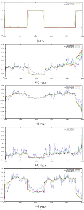
Figure 5 plots the smoothed states and smoothed variances from the models during a covariance breakdown episode. All elements of the volatility matrix are included in the comparison as well as the correlation coefficient. It is clear that the VDGARCH-B model is closer to the true volatility dynamics in general, and particularly so during the breakdown period. The VDGARCH model has conditional moments that are more erratic and deviate from the truth.
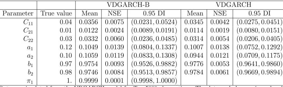
Table 3 repeats the exercise by estimating the models on simulated data with no covari-ance breakdowns. Here data are simulated from a plain VDGARCH model with parameters specified earlier and both specifications are estimated. The VDGARCH-B model does a good job in identifying no breakdowns and recovering the model parameters.
To quantitatively compare the fit of the models based on the volatility estimates in the presence of covariance breakdowns, we calculate the root mean squared error (RMSE) and report it in Table 4. Over the whole sample the VDGARCH-B model has aRM SE of 0.230
11
and the VDGARCH model has a RM SE of 0.630. Modeling the covariance breakdowns is important for accurate volatility estimation. Focusing only on the RMSE from covariance breakdown periods ({t|st= 2}) the results show that both models have a higher value but the
loss from ignoring the covariance breakdowns is larger. The final columns of the table report the model losses when the data generating process contains no breakdowns (st= 1,∀t).
Ignoring covariance breakdowns results in biased parameter estimates and poor volatility estimates.
5
Marginal Likelihood
The marginal likelihood is a key input in Bayesian model comparison. It is defined as the integral of the likelihood function with respect to the prior density. Our approach to computing the marginal likelihood is based on the method proposed by Chib (1995), which exploits the fact that the marginal likelihood can be expressed as:
f(Y) = f(Y|Ψ)f(Ψ)
f(Ψ|Y) , (22)
where Ψ is the set of parameters,f(Y|Ψ) is the likelihood function,f(Ψ) andf(Ψ|Y) are the prior density and posterior density of the parameters, respectively. Equation (22) is called the basic marginal likelihood identity. It holds for any Ψ, but is most efficiently estimated at some high density point Ψ∗, such as the posterior mean or median. Calculation of the marginal
likelihood amounts to computing three quantities: f(Y|Ψ∗), f(Ψ∗) and f(Ψ∗|Y). After
evaluating the three quantities at some given parameter value Ψ∗, the marginal likelihood
on the log scale can be estimated as
logf(Y) = logf(Y|Ψ∗) + logf(Ψ∗)−logf(Ψ∗|Y). (23)
To estimate logf(Y|Ψ∗) the latent state variables S and Λ are integrated out of the
likelihood function. We design a particle filter based on the auxiliary particle filter of Pitt & Shephard (1999) to achieve this purpose for our model. The second term, logf(Ψ∗), is the
log-prior evaluated at Ψ∗. This is straightforward to compute given our priors. However,
simulations are used to calculate integrating constants from prior restrictions such asπ1 > π2.
The final term, logf(Ψ∗|Y), is the log-posterior ordinate. We follow Chib & Jeliazkov (2001),
who provide an approach that can be used for M-H sampling steps while Chib (1995) can be used for the Gibbs sampling steps. Full details of the marginal likelihood estimation are found in Section 8.3.
6
Empirical Application
In this section we apply the model to study the volatility dynamics among the stock market and the bond market.12 We use daily excess returns on the S&P 500 index (y
1,t), a ten-year
12For applications of MGARCH models to stock and bond markets without covariance breakdowns see
Treasury bond (y2,t), and a one-year Treasury bond (y3,t). The return data are obtained
from the Center for Research on Security Prices (CRSP). The excess returns are obtained by subtracting the risk-free return approximated by the three-month Treasury bill rate. The sample period runs from 1987/01/02 to 2011/12/30, delivering 6244 observations. Figure 6 plots the three excess return series and Table 5 provides summary statistics. Returns are in percentage.
We estimate the VDGARCH-B model and the VDGARCH-t-B model using the return data. For the GARCH parameter Θ, the priors on the elements ofa,b,C are all independent N(0,100), except that a1, b1 and the diagonal elements of C are truncated to be positive for
identification purposes. The other prior distributions are set as follows: ν∼Expν>k−1(0.1),
an exponential distribution with support truncated to be greater thank−1;Q0 ∼W(5, I), a
Wishart distribution with 5 degrees of freedom and scale matrix equal toI;µ∼N(0,100I). The degree of freedom of the Student-t distribution in VDGARCH-t-B follows a truncated exponential distribution, d∼Expd>2(0.1).
The priors of π1 and π2 are set with απ1 = 20, βπ1 = 0.1, απ2 = 2, βπ2 = 0.1 and favor
infrequent covariance breakdowns. To ensure that covariance breakdowns are meaningful and not just capturing outliers the posterior sampling of st is restricted to span a minimum
duration of D days for each state (normal and breakdown). The original case corresponds with D = 1. In this analysis, we set D = 5 which represents a normal business week.13 Finally, the restriction of π1 > π2 ensures normal periods dominate breakdown periods so
that the GARCH dynamics would prevail in the long-run, serving as the main driving force of volatility dynamics. The first 10000 draws of the MCMC chain are discarded as burn-in and the next 10000 draws are used for inference.
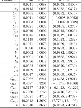
First, we discuss the VDGARCH-B model. The parameter estimates are reported in Table 6. Figure 7a plots the posterior mean of st. A visual inspection suggests that a large
number of breakdown periods are identified by the model. The posterior average number of breakdown periods is 199. The posterior average of the breakdown period duration is 14 days. The top panel of Table 7 shows the empirical posterior distribution of the duration of the breakdown periods (state 2 duration). More than 88% of the breakdown periods have a duration of less than or equal to 30 days. 14% of the breakdown periods have the minimum duration of 5 days. Figure 7b plots the posterior mean of log(|Λt|). Recall that log(|Λt|)>0
(log(|Λt|) < 0) means a scale-up (scale-down) effect on the volatility matrix. The figure
shows that log(|Λt|) > 0 most of the time. This suggests during most of the breakdown
periods, the overall variability is scaled up. The above results indicate that many short-lived breakdown periods occur to scale up the volatility in order to pick up tail realizations of the return distribution.
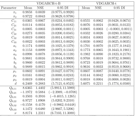
Next, we turn our attention to the VDGARCH-t-B model. The parameter estimates are reported in Table 8. Relative to Table 6, the notable difference is that with the t-distribution both π1 and π2 have much higher estimated values. This means that state durations will
tend to be longer with fewer breakdown periods (and normal periods). This is evident in the plot of the posterior mean of st in Figure 8a. The posterior average number of breakdown
periods is 44, less than one fourth of the number in the Gaussian case. The breakdown periods cover less days. The posterior average number of days in state 2 is 2282, accounting
for 36% of the total sample. The posterior average duration of a breakdown is 58 days, four times in length as compared to the Gaussian case.
The empirical posterior distribution of the duration of the breakdown periods is shown in the bottom half of Table 7. More than 30% of the breakdown periods have durations of more than 60 days and on average only 2 breakdown periods have the minimum duration of 5 days. According to the estimates of the Markov chain parameters π1 and π2 in Table 8,
covariance breakdowns occur 34% of the time and their expected duration is 1-2 months. Evidently, there is a substitution effect between the t-distribution and Λt. A large number
of those short-lived breakdown periods with jumps in the overall variability with Gaussian innovations are classified as tail observations under the fat-tailed Student-t assumption. A fat-tailed innovation distribution is important in separating transient outliers from sustained covariance breakdowns.
Figure 8a also shows clusters of breakdown periods at the beginning, in the middle part and also towards the end of the whole sample. Some of these are discussed later. Figure 8b plots the posterior mean of log(|Λt|). When there is likely a normal state indicated by the
posterior mean ofst, log(|Λt|) is close to one as it should be; while during breakdown periods,
log(|Λt|) have both positive and negative values. This means that the model has identified
both breakdown periods with overall increased variability and those with reduced variability. Table 9 reports posterior summary statistics for the expected impact of covariance downs. The posterior mean of 0.5808 implies an average increase in variability when a break-down occurs. However, the 0.95 density interval shows that reductions in variability do occur (a negative value of log(|E[Λ]|) implies a decrease in the generalized variance). The density interval shows that the distribution of expected breakdowns is asymmetric in that increases in variability are much more likely than decreases.
We also estimate a plain VDGARCH model with Student-t innovations
(VDGARCH-t)14. See Table 8 for parameter estimates. Compared to VDGARCH-t-B, VDGARCH-t
has larger estimates of ai. Meanwhile, the estimate of the degree of freedom d is smaller,
evidence of the substitution effect between the t-distribution and covariance breakdowns.
6.1
Model Comparison
To formally assess whether covariance breakdowns admitted in our model are supported by the data, we compute the marginal likelihoods and compare models based on Bayes factors. The marginal likelihood for the covariance breakdown specifications is evaluated as discussed in Section 5.
Computing the marginal likelihood for the models without covariance breakdowns is straightforward using the method in Chib & Jeliazkov (2001), where evaluating the likelihood function and the prior ordinates is trivial, and the posterior ordinate can be evaluated using a single block proposal within M-H steps.
Table 10 reports the results for several MGARCH specifications with Gaussian and Student-t innovations, and with or without covariance breakdowns. The final column of the table reports the log-Bayes factor (the difference of the log marginal likelihoods of the two
14The prior distributions for the parameters are the same as those for the common parameters in
models) for the VDGARCH-t-B against each of its alternatives. This model is strongly fa-vored against all alternatives. Adding covariance breakdowns improves each MGARCH spec-ification. The log Bayes factor in favor of the VDGARCH-t-B model versus the VDGARCH-t is 59.575, which is overwhelming evidence.15
6.2
Covariance Breakdown Episodes
In this section we discuss several identified covariance breakdowns from the VDGARCH-t-B model. In particular, we compare the volatility dynamics under the full specification which includes the impact of the breakdownVt=Ht1/2Λt(Ht1/2)
′
against the MGARCH component Ht, of the model.
6.2.1 2001-2005
The first episode is between 2001/01/02 and 2005/12/30 and found in Figure 9. Two adjacent extended breakdown periods are identified (Figure 9a). Together they span over one year in time from May 2002 to May 2003, a period featuring significant stock market downturn after the “Internet bubble bursting”. The first breakdown period finishes at around mid October 2002 and the second period starts about a week later. Although the two periods occur closely in time they are distinguished from each other, evident by the large difference in log(|Λt|). In both periods log(|Λt|) <0, indicating overall reduced variability relative to
Ht. During these breakdowns we see a large deviation between the conditional moments of
Vt and Ht.
The first breakdown period witnesses the bankruptcy case of WorldCom.16 This
covari-ance breakdown results in significant jumps in the conditional varicovari-ances of the S&P 500 and the ten-year bond while the one-year bond decreases relative to Ht. There are large drops
in the conditional covariances of excess returns between the stock and bond markets. These changes cause substantial drops in conditional correlations. For instance, the conditional correlation between S&P 500 and the ten-year bond drops from about 0 to below -0.6 with a similar effect between the stock market and the one-year bond. On the other hand, the conditional correlation on excess returns from the bond markets spike to well above 0.7.
The second breakdown is from November 2002 to April 2003. The main effect is on the conditional variance of the one-year bond which drops to lower levels than Ht. This results
in a reduction in the conditional correlation between S&P and the one-year bond (Figure 9i) and an increase between the two bonds (Figure 9j). Note, that the apparent breakdowns in these correlations have their source in the drop of the conditional variance of the one-year bond and not covariances, since the conditional covariances are very close to those from Ht
(after November 2002). Immediately after the end of the second breakdown both Htand Vt
are essentially the same.
15Kass & Raftery (1995) suggest interpreting the evidence for model Aas: not worth more than a bare
mention if 0≤log(BFAB)<1; positive if 1≤log(BFAB)<3; strong if 3≤log(BFAB)<5; and very strong
if log(BFAB)≥5.
16On May 9, 2002, Standard & Poor’s and Moody’s cut WorldCom’s credit rating to junk status. On July
In summary, during this period we have covariance breakdowns that impact conditional variances, covariances and correlations.
6.2.2 2008-2011
The second episode is from 2008/01/02 to 2011/12/30 and is found in Figure 10. This in-cludes the recent financial crisis of 2008. Not surprisingly, two consecutive sustained break-down periods are identified by the model starting from September 2008 until November 2009 while there are shorter breakdowns in 2010 and 2011. The first breakdown period lasts for three months. During this period the covariance breakdown implies an increase in overall variability of exp(2.7)≈15 times.17
Some of the covariance breakdowns over this sample period increase variability while some decrease it. The differences in the conditional variances and covariances of Vt and Ht
are more pronounced than the differences between the conditional correlations. In other words, these are covariance breakdowns that have little to no impact on the conditional correlations. Relative to Ht, there is no evidence of a correlation breakdown in Vt.
6.2.3 1987-1989
The final episode is from 1987/01/02 to 1989/12/30 and is plotted in Figure 11. This features the stock market crash in October of 1987, which is within a one-month breakdown period identified by the model.
The main feature of this period is the large increase in conditional variances of all excess returns. The breakdown model implies at least a doubling of the conditional variances compared to those from Ht. The second breakdown after the crash provides a relief valve
that puts the breakdown variances below those ofHt. This allows for a faster return to normal
levels of volatility. The conditional covariances show a spike associated with the crash and these translate into sustained breakdowns in the conditional correlations between stock and bond markets. There is no evidence of a breakdown in the conditional correlation of excess returns between the two bonds. In other words, the spikes in the conditional variances and covariance in the bond market largely cancel out in the conditional correlation.
The covariance breakdown model is flexible enough to capture complex and erratic tem-porary structural change/deviation from the long run volatility dynamics which is otherwise difficult to account for comprehensively. It provides a relief value to release the excessive volatility built into MGARCH models after a shock as well as a mechanism to capture abrupt increases/decreases in variance, covariance and correlation dynamics.
6.3
Portfolio Choice
We evaluate the out-of-sample performance of the models from a portfolio optimization perspective. We consider a risk-averse investor who allocates funds among three risky assets, namely, the stock market portfolio, the ten-year bond, the one-year bond, and the risk-free asset. The investor bases her decision on the mean-variance criterion and rebalances her
17
portfolio daily using a volatility-timing strategy. Specifically, at each day t, she solves for the minimum variance portfolio subject to a required return constraint:
min
wt+1
w′
t+1Σt+1wt+1, (24)
s.t. wt′+1µ=µ0. (25)
wt+1 is the 3×1 vector of portfolio weights to be chosen at time t, Σt+1 is the one-period
ahead forecast of the timet+1 covariance matrix ofyt+1,µis the assumed vector of expected
excess returns over the risk-free return, and µ0 is the required (target) portfolio return in
excess of the risk-free return. The solution renders the optimal portfolio weight
wt+1 =
Σ−t+11µ µ′Σ−1
t+1µ
µ0. (26)
The realized portfolio return (in excess of the risk-free rate) is given by
Rt+1 =wt′+1yt+1. (27)
Note that P3i=1wt,i will not equal one in general, and 1−P3i=1wt,i is the share invested in
the risk-free asset.
To evaluate the economic gains of allowing for covariance breakdowns in the MGARCH volatility dynamics in the context of portfolio selection, we use the utility-based approach following Fleming et al. (2001) and Clements & Silvennoinen (2013). Let {R1t}Tt=T0 be
the realized portfolio returns over the out-of-sample period using volatility forecasts based on the VDGARCH-t model, and {R2t}Tt=T0 be those based on the covariance breakdown
(VDGARCH-t-B) model. 18 Given a utility functionU(.), we find a constant ∆ that equates
the total realized utility in
T
X
t=T0
U(R1t) = T
X
t=T0
U(R2t−∆). (28)
∆ is the daily maximum return the investor would be willing to give up in exchange for the economic gains obtained by switching from the model with no covariance breakdowns to one with breakdowns. As such, ∆ measures the incremental benefit of allowing for covariance breakdowns as opposed to otherwise. A positive value of ∆ means that allowing for covariance breakdowns will generate extra economic benefit for the investor. Here we consider two types of utility functions. One is the quadratic utility function in Fleming et al.(2001, 2003)
Uq(Rt) = (1 +rf t+Rt)−
τ
2(1 +τ)(1 +rf t+Rt)
2, (29)
and the other is the negative exponential utility used in Clements & Silvennoinen (2013) and Skouras (2007)
Ue(Rt) = −exp(−τ(1 +rf t+Rt)). (30)
18The forecasts of Σ
t+1 are computed using parameter estimates conditioning on information up to time
rf t is the risk-free return and τ is the investor’s coefficient of risk aversion.
To focus on the difference that volatility dynamics make we demean the data and estimate the models with a zero intercept, and we setµin (25) to be the sample mean for both models. Any differences in portfolio choice are directly related to the differences in the covariance dynamics. We consider two out-of-sample periods. The first sample period focuses on the financial crisis while the second is extended to a longer period prior to the crisis. Table 11 reports the results for portfolio performance from the covariance timing strategies for several required return valuesµ0. Overall, an investor is willing to pay for the covariance breakdown
model. It achieves a higher Sharpe ratio in both samples. The performance fee is largest for larger µ0. These results show that the superior predictability of the covariance breakdown
model translates into economic gains in portfolio choice.
7
Conclusion
This paper proposes a flexible way of accommodating dynamic heterogeneous breakdown pe-riods in the conditional covariance matrix of multivariate GARCH models. During pepe-riods of normal market activity, volatility dynamics are governed by an MGARCH specification. A covariance breakdown is any significant temporary deviation of the conditional covariance matrix from its implied MGARCH dynamics. This is captured through a flexible stochas-tic component that allows for changes in the conditional variances, covariances and implied correlation coefficients. Bayesian inference is used and we propose an efficient posterior sam-pling procedure. We show how to compute the marginal likelihood of our model. Application in daily stock and bond return data shows the benefit of our approach. The new model is strongly supported by Bayes factors while gains to portfolio choice are also documented.
8
Appendix
8.1
Derivation of Equation (7)
We compute the integralR (Qnt=1p(yt|Λ))p(Λ)dΛ for somen≥1 where Λ ∼W−1(ν, Q0) and
yt∼N ID(0,Λ). First note that
n
Y
t=1
p(yt|Λ)
!
=
n
Y
t=1
1 (2π)k2|Λ|
1 2
exp
−1
2y
′
tΛ−1yt
= (2π)−nk2 |Λ|−
n
2 exp −1
2
n
X
t=1
y′tΛ−1yt
!
= (2π)−nk2 |Λ|−
n
2 exp −1
2
n
X
t=1
T r(y′tΛ−1yt)
!
= (2π)−nk2 |Λ|−
n
2 exp −1
2
n
X
t=1
T r(Λ−1yty′t)
!
Therefore,
n
Y
t=1
p(yt|Λ)
!
p(Λ) = (2π)−nk2 |Λ|−
n
2 exp −1
2
n
X
t=1
T r(Λ−1ytyt′)
!
× |Q0|
ν
2|Λ|−
ν+k+1 2
2νk2 Qk j=1Γ(
ν+1−j
2 )
exp
−1
2T r(Λ
−1Q 0)
= (2π)−
nk
2 |Λ|−
n+ν+k+1 2 |Q0|
ν
2
2νk2 Qk j=1Γ(
ν+1−j
2 )
exp −1
2T r[Λ
−1(
n
X
t=1
ytyt′ +Q0)]
!
= |Q|
n+ν
2 |Λ|−
n+ν+k+1 2
2(n+2ν)k Qk j=1Γ(
n+ν+1−j
2 )
exp
−1
2T r(Λ
−1Q)
×2
nk
2 (2π)−
nk
2 |Q0|
ν
2 Qk j=1Γ(
n+ν+1−j
2 )
|Q|n+2νQk j=1Γ(
ν+1−j
2 )
= W−1(Λ|n+ν, Q)× 2
nk
2 (2π)−
nk
2 |Q0|
ν
2 Qk j=1Γ(
n+ν+1−j
2 )
|Q|n+2ν Qk j=1Γ(
ν+1−j
2 )
(31)
where Q = Pnt=1ytyt′ +Q0. So integrating this final result with respect to Λ leaves the
second term on the right hand side of (31) since the first term is a well defined inverse-Wishart density that integrates to 1. That is,
Z Yn
t=1
p(yt|Λ)
!
p(Λ)dΛ = 2
nk
2 (2π)−
nk
2 |Q0|
ν
2 Qk j=1Γ(
n+ν+1−j
2 )
|Q|n+2ν Qk j=1Γ(
ν+1−j
2 )
. (32)
8.2
Sampling
ν
and
Q
0Forν, the conditional posterior distribution is
p(ν|Y, Q0,Θ, µ,S) ∝ p(Y|Θ, µ, ν,S, Q0)p(ν)
∝ p( ˜Y|S, Q0, ν)p(ν)
∝
B
Y
q=1
|Q0| ν
2 Qk j=1Γ(
Nq+ν+1−j
2 )
|Qq|
ν
2 Qk j=1Γ(
ν+1−j
2 )
!
p(ν). (33)
The prior ofνis an exponential distribution with support truncated to be greater thank−1, p(ν) ∝ Exp(ν|λ1)Iν>k−1. Sampling from p(ν|Y, Q0,Θ,S) can be achieved by an M-H step
with a random walk proposal.
scalar degree of freedom γ0 and scale matrix A. then
p(Q0|ν,{Λ˜q}Bq=1) ∝ p({Λ˜q}Bq=1|Q0, ν)p(Q0)
∝
B
Y
q=1
|Q0| ν
2 exp(−1
2T r(˜Λ
−1
q Q0))
!
|Q0| γ0−k−1
2 exp(−1
2T r(A
−1Q 0))
∝ |Q0| Bν
2 exp −1
2T r(
B
X
q=1
˜ Λ−q1Q0)
!
× |Q0| γ0−k−1
2 exp(−1
2T r(A
−1Q 0))
∝ |Q0|
Bν+γ0−k−1
2 exp −1
2T r (
B
X
q=1
˜
Λ−q1+A−1)Q0
!!
∝ Wk(Q0|γ,A)e (34)
where γ =Bν+γ0,Ae= (PBq=1Λ˜−q1+A−1)−1.
8.3
Marginal Likelihood Estimation
Below the estimation of each of the components of (23) is provided.
8.3.1 Estimating f(Y|Ψ)
We assume Student-t innovation for the data:19
yt∼t(µ, Ht1/2Λt(Ht1/2)′, d).
The parameter set Ψ includes Θ, µ, π1, π2, d, ν, Q0. Write ˜Yt={y˜t}tT=1 and ˜yt=Ht−1/2(yt−µ).
Note that
f(Y|Ψ) =
" T Y
t=1
|Ht|−1/2
#
f( ˜Y|π1, π2, d, ν, Q0). (35)
The likelihood function can be obtained by computing QTt=1|Ht|−1/2 and f( ˜Y|Ψ1), where
Ψ1 ={π1, π2, d, ν, Q0}. ComputingQTt=1|Ht|−1/2 is straightforward given Θ andµ. f( ˜Y|Ψ1)
is the likelihood function of the transformed data ˜Y. It can be shown that ˜Y correspond with the following “transformed” model:
˜
yt|Λt ∼ t(0,Λt, d) (36)
Λt|(Λt−1 =I)
=I with probability π1
∼W−1(ν, Q
0) with probability 1−π1 (37)
Λt|(Λt−1 6=I)
= Λt−1 with probability π2
=I with probability 1−π2 (38)
19For the case of Gaussian innovations, the likelihood function can be obtained in a similar and simpler
Once again using the fact that a Student-t random variable can be written as a ratio of a Gaussian variable and the square root of a Gamma random variable, the model can be further converted into a conditionally Gaussian state space model:
˜
yt|Λt, ut ∼ N(0, u−t1Λt) (39)
Λt|(Λt−1 =I)
=I with probability π1
∼W−1(ν, Q
0) with probability 1−π1 (40)
Λt|(Λt−1 6=I)
= Λt−1 with probability π2
=I with probability 1−π2 (41)
ut iid∼ G(d/2, d/2) (42)
The state variables are (Λt, ut). The transformed likelihood function can be written as
f( ˜Y|Ψ1) =
T
Y
t=1
f(˜yt|Yt˜ −1,Ψ1) =
T
Y
t=1
Z
f(˜yt|Λt, ut)f(Λt, ut|Yt˜ −1,Ψ1)d(Λt, ut), (43)
where ˜Yt={y˜i}ti=1. To approximate the likelihood function, we design an Auxiliary Particle
Filter (APF) (Pitt & Shephard 1999) to sequentially sample from the filtering distribution f(Λt, ut|Yt˜ ,Ψ1),t = 1, . . . , T. Given M particles {(Λ(tj), u
(j)
t )}Mj=1 fromf(Λt, ut|Yt˜ ,Ψ1), each
with the same discrete probability mass 1/M and suppressing Ψ1 from the conditioning set,
the predictive density is
f(Λt+1, ut+1|Yt˜ ) =
Z
f(Λt+1, ut+1|Λt, ut)f(Λt, ut|Yt˜ )d(Λt, ut)
=
Z
f(ut+1)f(Λt+1|Λt)f(Λt, ut|Y˜t)d(Λt, ut)
≈ f(ut+1)
M
X
j=1
f(Λt+1|Λ(tj))
1
M. (44)
Therefore
f(Λt+1, ut+1|Yt˜ +1)∝f(˜yt+1|Λt+1, ut+1)f(ut+1)
M
X
j=1
f(Λt+1|Λ(tj)). (45)
To sample fromf(Λt+1, ut+1|Y˜t+1), introduce an auxiliary discrete variablem∈ {1, . . . , M}
and define
f(Λt+1, ut+1, m|Yt˜ +1)∝f(˜yt+1|Λt+1, ut+1)f(ut+1)f(Λt+1|Λ(tm)). (46)
If we draw from this joint distribution in (46) and then discard the indexm, we will produce a sample from the distribution in (45).
To sample from f(Λt+1, ut+1, m|Yt˜ +1), we use Gibbs steps to iteratively sample from the
conditional distributions off(ut+1|Λt+1, m,Yt˜ +1) and f(Λt+1, m|ut+1,Yt˜ +1). Note that
f(ut+1|Λt+1, m,Yt˜ +1) ∝ f(˜yt+1|Λt+1, ut+1)f(ut+1)
∝ G ut+1
k+d
2 ,
d+ ˜y′
t+1Λ−t+11 y˜t+1
2
!
where G(.|., .) is the Gamma probability density function. We discuss the sampling of f(Λt+1, m|ut+1,Yt˜ +1) in detail:
• Case I: If Λ(tm) =I
f(˜yt+1|Λt+1, ut+1)f(Λt+1|Λ(tm)) =
N(˜yt+1|0, ut−+11 I)π1 if Λt+1 =I
N(˜yt+1|0, u−t+11 Λt+1)W−1(Λt+1|ν, Q0)(1−π1) if Λt+1 6=I. (48)
Thus we have
P r(Λt+1 =I|Yt˜ +1,Λ(tm) =I, ut+1) ∝ N(˜yt+1|0, u−t+11 I)π1 (49)
P r(Λt+1 6=I|Yt˜ +1,Λ(tm) =I, ut+1) ∝
Z
N(˜yt+1|0, λ−t+11 Λt+1)W−1(Λt+1|ν, Q0)dΛt+1(1−π1)
= Π
−k
2u
k
2 t+1|Q0|
ν
2 Qk j=1Γ(
ν+2−j
2 )
|Q˜t+1|
1+ν
2 Qk j=1Γ(
ν+1−j
2 )
(1−π1), (50)
where ˜Qt+1 =ut+1y˜t+1y˜t′+1+Q0. Define
gm(˜yt+1, ut+1) = N(˜yt+1|0, u−t+11 I)π1+
Π−k
2u
k
2 t+1|Q0|
ν
2 Qk j=1Γ(
ν+2−j
2 )
|Q˜t+1|
1+ν
2 Qk j=1Γ(
ν+1−j
2 )
(1−π1). (51)
• Case II: If Λ(tm)6=I
f(˜yt+1|Λt+1, ut+1)f(Λt+1|Λ(tm)) =
N(˜yt+1|0, ut−+11I)(1−π2) if Λt+1 =I
N(˜yt+1|0, u−t+11Λ (m)
t )π2 if Λt+1 = Λ(tm).
(52)
In this case, define
gm(˜yt+1, ut+1) = N(˜yt+1|0, ut−+11 I)(1−π2) +N(˜yt+1|0, u−t+11 Λ (m)
t )π2. (53)
Putting this together, to sample fromf(Λt+1, m|Yt˜ +1, ut+1), first sample the indexmwith
probability in proportion togm(˜yt+1, ut+1). Givenm, 1) if Λt(m) 6=I, then Λt+1 =I or Λt+1 =
Λ(tm), with probability in proportion to N(˜yt+1|0, u−t+11 I)(1−π2) and N(˜yt+1|0, u−t+11 Λ (m)
t )π2,
respectively (see equation (52)). 2) If Λ(tm) =I, then Λt+1 =I or Λt+1 6=I, with probability
in proportion to N(˜yt+1|0, u−t+11 I)π1 and
Π−k2uk2
t+1|Q0|
ν
2Qkj=1Γ(ν+2−2 j)
|Q˜t+1| 1+ν
2 Qkj=1Γ(ν+1−2 j) (1−π1), respectively
(equa-tion (49) and (50)); given Λt+1 6= I, sample Λt+1 from the distribution W−1(ν + 1,Q˜t+1),
where ˜Qt+1 =ut+1y˜t+1y˜t′+1+Q0.
Use the above method to sampleM draws of (Λ(tj+1) , m(j), u (j)
t+1),j = 1, . . . , M. {(Λ (j)
t+1, u (j)
t+1)}Mj=1
constitute a sample from f(Λt+1, ut+1|Y˜t+1) and are the desired particles.
Given the above filtering procedure, the likelihood is estimated using the decomposition f( ˜Y|Ψ1) =QTt=1f(˜yt|Yt˜ −1,Ψ1):
2. For each Λ(t−j)1, sample Λ(tj)|Λ
(j)
t−1 according to the transition distribution defined in (37)
and (38).
3. Approximate f(˜yt|Yt˜ −1,Ψ1) as ˆf(˜yt|Yt˜ −1,Ψ1) = M1 PMj=1t(˜yt|0,Λ(tj), d), wheret(.|., ., .)
is the density of the Student-t distribution.
Repeat the above steps for each t, and estimate logf( ˜Y|Ψ1) by PTt=1log ˆf(˜yt|Yt˜ −1,Ψ1).
8.3.2 Estimating f(Ψ|Y)
To compute the posterior ordinate at some Ψ∗, we use the method of Chib & Jeliazkov
(2001). Write
f(Ψ∗|Y) = f(Θ∗|Y)×f(µ∗|Y,Θ∗)×f(π1∗, π2∗|Y,Θ∗, µ∗)×f(d∗|Y,Θ∗, µ∗, π1∗, π∗2) ×f(ν∗|Y,Θ∗, µ∗, π∗1, π2∗, d∗)×f(Q0∗|Y,Θ∗, µ∗, π1∗, π∗2, d∗, ν∗). (54)
As described in Section 3, each block of the parameters is sampled using an M-H step, except for Q0, which is sampled using a Gibbs step. To estimate f(Θ∗|Y), denote by q(Θ,Θ∗) the
proposal density for the transition from Θ to Θ∗ and byα(Θ,Θ∗|Y, µ, ν, Q
0,S,U) the M-H
probability to move. Using the results from Chib & Jeliazkov (2001), the ordinatef(Θ∗|Y)
can be expressed as
f(Θ∗|Y) =
R
α(Θ,Θ∗|Y, µ, ν, Q
0,S,U)q(Θ,Θ∗)f(Θ, µ, ν, Q0,S,U|Y)d(Θ, µ, ν, Q0,S,U)
R
α(Θ∗,Θ|Y, µ, ν, Q0,S,U)q(Θ∗,Θ)f(µ, ν, Q0,S,U|Y,Θ∗)d(Θ, µ, ν, Q0,S,U) (55)
The numerator can be estimated as
1 M
M
X
j=1
α(Θ(j),Θ∗|Y, µ(j), ν(j), Q0(j),S(j),U(j))q(Θ(j),Θ∗), (56)
where (Θ(j), µ(j), ν(j), Q(j)
0 ,S(j),U(j)) is from the jth draw of the full MCMC run of the
pos-terior distribution f(Ψ,S,U,Λ|Y), which consists of {Θ(j), µ(j), π(j) 1 , π
(j)
2 , d(j), ν(j), Q (j) 0 ,
S(j),U(j),Λ(j)}. For the denominator, the integral is with respect to the distribution
f(µ, ν, Q0,S,U|Y,Θ∗) ×q(Θ∗,Θ). To estimate this integral, fix Θ at Θ∗ and conduct a
reduced run of another M iterations sampling the conditional posterior distributions of all the state variables (S,U,Λ) and parameters except Θ. At each iteration of the reduced run, also draw Θ from the proposal density q(Θ∗,Θ). The results will provide M draws
of {µ(l), ν(l), Q(l)
0 ,S(l),U(l),Θ(l)} from the distribution f(µ, ν, Q0,S,U|Y,Θ∗)q(Θ∗,Θ). Then
the denominator is estimated as
1 M
M
X
l=1
α(Θ∗,Θ(l)|Y, µ(l), ν(l), Q(0l),S(l),U(l)). (57)
The ordinate f(µ∗|Y,Θ∗) can be expressed as
f(µ∗|Y,Θ∗) =
R
α(µ, µ∗|Y,Θ∗, d,Λ)q(µ, µ∗)f(µ, d,Λ|Y,Θ∗)d(µ,Λ, d) R
The numerator can be estimated as
1 M
M
X
j=1
α(µ(j), µ∗|Y,Θ∗, d(j),Λ(j))q(µ(j), µ∗), (59)
where (µ(j), d(j),Λ(j)) is from thejthdraw of the reduced MCMC run of the posterior
distribu-tion with Θ fixed at Θ∗, which were used in the previous step to estimate the denominator in
(55). For the denominator in (58), the integral is with respect tof(d,Λ|Y,Θ∗, µ∗)×q(µ∗, µ).
To estimate this integral, fix Θ at Θ∗ and µat µ∗, and conduct a second reduced run of M
iterations sampling the conditional posterior distributions of all the state variables and pa-rameters except Θ andµ. At each iteration, drawµfrom the proposal densityq(µ∗, µ). The
results will provideM draws of (µ(l), d(l),Λ(l)) from the distributionf(d,Λ|Y,Θ∗, µ∗)q(µ∗, µ).
The denominator is estimated as
1 M
M
X
l=1
α(µ∗, µ(l)|Y,Θ∗, d(l),Λ(l)). (60)
The ordinate f(π∗
1, π∗2|Y,Θ∗, µ∗) can be expressed as
f(π1∗, π2∗|Y,Θ∗, µ∗) =
R
α(π, π∗|S)q(π∗|S)f(π,S|Y,Θ∗, µ∗)d(S, π) R
α(π∗, π|S)q(π|S)f(S|Y,Θ∗, µ∗, π∗)d(S, π), (61)
where π = {π1, π2}. q(.|S) is the density of the independent proposal which does not use
the last iteration in the proposal of a new value of π, but depends on the value of S. The numerator can be estimated as
1 M
M
X
j=1
α(π(j), π∗|S(j))q(π∗|S(j)), (62)
where (π(j),S(j)) is from the jth draw of the second reduced MCMC run of the posterior
distribution with Θ fixed at Θ∗ and µ fixed at µ∗, used in the previous step to estimate
the denominator of (58). To estimate the integral in the denominator of (61), fix Θ, µ, π at Θ∗, µ∗, π∗, respectively, and conduct a third reduced run of M iterations sampling the
conditional posterior distributions of all the state variables and parameters except Θ,µandπ. At each iteration l, given the value ofS(l), draw π(l) from the proposal density q(.|S(l)). The
resulting (S(l), π(l)), l = 1, . . . , M are draws from the distribution f(S|Y,Θ∗, µ∗, π∗)q(π|S).
The denominator is estimated as
1 M
M
X
l=1
α(π∗, π(l)|S(l)). (63)
The ordinate f(d∗|Y,Θ∗, µ∗, π∗
1, π∗2) can be expressed as
f(d∗|Y,Θ∗, µ∗, π1∗, π2∗) =
R
α(d, d∗|U)q(d, d∗)f(d,U|Y,Θ∗, µ∗, π∗)d(U, d) R