An Accurate and Eﬃcient Computation of Zeros and Poles of Transfer Function for Large Scale Circuits

(1)

An Accurate and Efficient Computation of Zeros and

Poles of Transfer Function for Large Scale Circuits

Josef Dobeš, Jan Míchal, František Vejražka, and Viera Biolková

Abstract—The zeros and poles of a circuit transfer function are computed solving a general eigenvalue problem, which could be transformed to a standard eigenvalue task to be solved by a suitably modified QR algorithm. Both reduction of the general eigenvalue problem to the standard form and the iterative pro-cedures of the QR algorithm are very sensitive to the numerical precision of all calculations. The numerical accuracy is especially critical for two kinds of circuits: the microwave ones characterized by huge differences among magnitudes of the zeros and poles, and the large scale circuits, where the errors of the zeros and poles are increased by an extreme number of arithmetic operations. In the paper, an illustrative example of the reduction of the general eigenvalue problem and using the QR algorithm is shown first. After that, three circuits of various sizes are analyzed: simpler microwave low noise amplifier, larger power operational amplifier, and the most complex example with a 272 integrated operational amplifier. A meticulous comparison of obtained results shows that a usage of newly implemented 128-bit arithmetics in GNU Fortran or C compilers with partial pivoting can assure both efficient and enough accurate procedures for computing the zeros and poles.

Index Terms—large scale circuits, poles and zeros, general eigenvalue problem, numerical precision, 128-bit arithmetics.

I. Introduction

C

OMPUTING the poles and zeros of a circuit transfer function for sparse systems was principally described in [1]; however, the serious accuracy problem for the general eigenvalue problem remains for decades. Microwave circuits represent one typical problematic area [2], [3] due to huge differences in absolute values of their poles or zeros. Another typical problem consists in bad accuracy of computing multiple eigenvalues using the QR [4], [5] and QZ [6] algorithms. For the large scale circuits, besides these accuracy problems, the efficiency of math procedures [7], [8], [2] also has to be taken into account. Although for relatively simple microwave circuits some version of variable-length arithmetic ([3], e.g.) can be used, this way is inappropriate for the large circuits due to computing time. In this paper, we suggest using relatively new __float128GCC orreal(16)GFortran precisions with partial pivoting to solve the accuracy problem for the larger circuits.

II. Description of Math Procedures With an Example A. Reducing General Eigenvalue Problem to the Standard One

Circuit equations (linear, or linearized at an operating point for nonlinear circuits) are defined by the matrix equation [1]:

sD+E

x=z, (1)

wheresrepresents Laplace operator, theDandEmatrices are composed of circuit reactances and resistances, andxandzare Laplace images of circuit variables and/or sources, respectively [7]. Poles and zeros of a transfer function are computed solving

Manuscript received June 19, 2019; revised July 18, 2019. This paper has been supported by the Technology Agency of the Czech Republic under grants TE01020186 and TH02010981, and by the Czech Science Foundation under grant 18-21608S.

J. Dobeš, J. Míchal, and F. Vejražka are with the Department of Radio-electronics, Czech Technical University in Prague, Czech Republic (e-mails: {dobes, michal, vejrazka}@fel.cvut.cz).

[image:1.595.313.546.127.250.2]

V. Biolková is with the Department of Radioelectronics, Brno University of Technology, Czech Republic (e-mail: [email protected]).

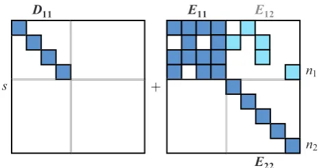
Fig. 1. Final forms of the matrices after the reduction of the general eigen-value problem to the standard one to be solved by the QR algorithm. The diagonalization ofD11andE22is obligatory. (In this case of shapes, there is no need to eliminateE12because its zeroing doesn’t change other matrices.)

det sD+E₌

0 for poles, (2a)

det sD(0l)+E(kl) =0 for zeros, (2b)

where the matrixD(0l)arises fromDby zeroing itslthcolumn,

and the matrix E(kl)arises fromE by replacing itslth column

by the vector zwith all its elements zeroed with the exception of the element corresponding to the kth input source.

A solution of the general eigenvalue problems (2) is more difficult than solving the standard one. Therefore, a systematic reduction (it doesn’t change eigenvalues) is applied transform-ing (2a) to the standard form shown in Fig. 1. (It is an improved alternative to [5]). After this transformation, we can go further:

det sD+E ₌ (−1)nl↔

n2 Ö

i=n1+1

E22i idet h

[image:1.595.310.548.685.772.2]

D11D11−1 | {z }

=1

sD11+E11 i

=(−1)nl↔

n1 Ö

i=1

D11i i

n2 Ö

i=n1+1

E22i idet s1+D11 −1_E

11 =0, (3)

wherenl↔is total number of the row and column interchanges

during the process, and1is unity matrix. Finally, determining the poles is finished by computing the eigenvalues of the matrix

Epoles0 =−D11−1E11. (4)

B. Illustrative Example of Calculating the Poles and Zeros Consider the circuit in Fig. 2, for which (1) gets the form

      

s© «

C −C

−C −C 2C

L ª ® ® ¬ +© « G G 1 −1 ª ® ® ¬        © « V1 V2 V3 I ª ® ® ¬ =© « VG ª ® ® ¬ (5) and the next sequence of the reduction operations is to be done:

(2)

• The first and second rows are added to the third row.

• The first and second columns are added to the third column.

• Exchange the third and fourth rows, and then the third and fourth columns.

• −1/2 multiple of the fourth column is added to the first, and −1/(2G) multiple of the fourth column is added to the third. After these operations, the matrix in (5) gets the form of Fig. 1:

s© « C C L ª ® ® ¬ +© «

G/2 −G/2 −1/2 G

−G/2 G/2 −1/2 G

1/2 1/2 1/(2G) −1 2G ª ® ® ¬ , (6)

therefore, the QR algorithm will be applied to the matrix (4):

E_poles0 =− 1/C

1/C

1/L

!

×

G/2 −G/2 −1/2

−G/2 G/2 −1/2

1/2 1/2 1/(2G)

!

.

(7) Evaluating (7) (G=1 mS,L=106.1033µH,C=53.05165 pF), and applying 25 iterations of the QR algorithm [8], we obtain

E0(25)

poles=

© «

−1.88496×107 −0.163957 −89.0719 −0.163957 −4.33837×107 −1.33285×1010 0.000885722 132537 3.86713×107

ª ® ¬

(8)

| {z }

≈0

with apparent two blocks: 1×1 (the upper left one), that gives the first pole p1 =−1.88496×107_{, and 2}_×_{2 (the lower right} one), that gives the second and third poles by the solution of

det

p₂_,₃+4.33837×107 1.33285×1010

−132537 p2,3−3.86713×107

=0 (9)

as p2,3 =−2.3562×106±9.12489×106j. (If we divide the first pole by−2π, we obtain the anticipated frequency 3×106Hz.) The second step is the calculation of the zeros. The matrix in (2b) is obtained by the Cramer’s rule for k=1 and l=2:

sD(02)+E(12)=s

© «

C −C

−C

−C 2C

L ª ® ® ¬ +© «

G V G

1 −1 ª ® ® ¬ , (10) and the next sequence of the reducing operations will be done:

• The first column is added to the third column.

• The first row is added to the third row.

• The third row is added to the second row.

• The second and fourth rows are exchanged, and then the second and fourth columns are exchanged.

• Subtract the fourth row from the first and third rows.

After these operations, (10) gets an alternative form of Fig. 1:

s© « C L C ª ® ® ¬ +© « −1 −1

G 1 G V G

ª ® ® ¬

, (11)

and the final matrix

Ezeros0 =

1/C

1/L

!

(12)

clearly has a triple zero eigenvalue, i.e.,z1,2,3 =0 as expected.

C. Extraordinary Movement: a Row from the Right to the Left

The transformation itself seems nothing else than a modifi-cation of the Gauss elimination method. However, an exception arises when the matrix D11 contains a nondiagonal element,

which is irreducible by any diagonal element of this matrix. In such case, a row from the lower part of the matrix is multiplied by the soperator, which is equivalent to moving a row of the

E22 matrix to the left. That nondiagonal element ofD11 can

then be easily reduced by means of this transferred row.

D. Various Pivoting Methods for the Reduction Algorithms

As the reduction process very often has problems due to the numerical accuracy, a full pivoting is preferred. Therefore, the nth key element is selected as (i.e., from the whole submatrix):

DnnBarg max

n5i5n2

n5j5n2 D_{i j}

,n=1, . . . ,n₂, (13a)

if |Dnn|5full max

15i<n|Din|, thenDnnB0. (13b)

For large scale circuits, the reduction algorithm has to be implemented with utilizing sparsity of the matrices. However, the application of the full pivoting is extremely difficult here from a programming point of view. Therefore, a partial piv-oting is mostly used in this case, and the nth key element is chosen from the rest of the nth column of the reduced matrix:

DnnBarg max

n5i5n2

|Din|,n=1, . . . ,n2, (14a)

if |D_nn|₅_sparse max

n<j5l

D_{n j}

, then D_nn_B0. (14b)

Detailed definition of the pivoting strategy and recognizing zero elements other than (13b) and (14b) are defined in [3].

E. Using the 128-bit Arithmetics (of GNU GCC and Fortran)

Although the pivoting methods described in Subsec. II-D improve overall properties of the poles-zeros analysis consider-ably, their precision is still insufficient for a number of circuits. Therefore, we have changed the standard 64-bit arithmetics to the newly implemented 128-bit (__float128) one, and, clearly many (previously problematic) tasks now work well. Moreover, as the GNU compilers have complete libraries for the 128-bit computing, changing the source code was relatively easy.

III. Testing Examples: Different Levels of Complexity For a clear demonstration how the 128-bit arithmetic can improve the accuracy, we performed the poles-zeros analysis for three practical electronic and microwave circuits of different levels of complexity. Both poles and zeros analyses have been performed for each circuit with both algorithms (partial pivoting, sparse matrix and total pivoting, full matrix) with the original 64-bit arithmetic and with the new 128-bit arithmetic. The partial pivoting sparse matrix case was also run with an arithmetic of a reference accuracy of 2048-bit mantissa, to which all the previous results have been related and compared in tables, ordered with growing order of magnitude. (For an easier orientation in frequency, all poles and zeros presented in tables were divided by 2π, i.e., their physical unit is Hz.)

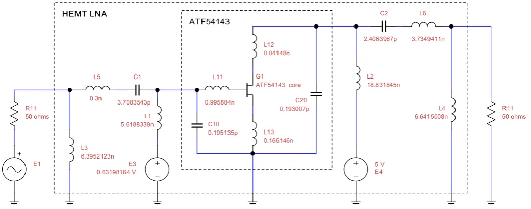
A. Low Noise Antenna Preamplifier (the simplest, microwave)

The first and simplest example is a radio-frequency circuit, a pHEMT LNA shown in Fig. 3. The analysis of the poles was unproblematic; however, in the zeros analysis, using the __float128precisions improved the accuracy considerably.

In the right column of Table I, the accurate zeros (the blue ones) are shown, which were computed with precise variable size arithmetic. (2048-bit was used – this one is extremely precise; however, it is unsuitable for large scale circuits because such computations may be extremely time-consuming.) For the DIFFERINGzeros, two phenomena arose, see the 1st– 4th column:

• For the partial pivoting, sparse matrix, double is completely wrong and __float128 makes it completely right to all six displayed figures – i.e.,__float128gave perfect results!

(3)

[image:3.595.39.560.51.256.2]

Fig. 3. Diagram of the low noise amplifier for a multiconstellation receiver of satellite navigation. The values were designed by the multiobjective optimization.

Fig. 4. Diagram of the AB-class power operational amplifier. This is the medium-complexity example of the tests of the accuracy with the results in Table II.

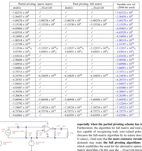
B. Discrete Power Operational Amplifier (medium complexity)

As a medium-complexity example, an AB-class discrete power operational example was analyzed, as shown in Fig. 4. Table II shows comparisons of poles and zeros in its 1stand 2nd parts, respectively. It is clear that the following observations can be made:

• Considering the case of partial pivoting and typedouble, poles that are different from the correct values differ only at the 6th significant place while some zeros differ at the 4th significant place.

• Using the__float128and using the full pivoting while keeping

doublehave both improved the accuracy of results to a similar extent.

• The use of __float128arithmetic improved accuracy for both poles and zeros, partial pivoting and full pivoting.

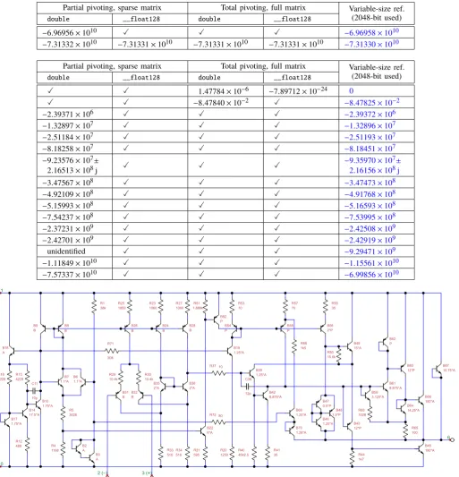
C. A 272 Integrated Operational Amplifier (the most complex)

The most complex example tried is an integrated operational amplifier of the 272 type. For running the PZ analysis on circuit in Fig. 5, the testbench circuit in Fig. 6 was used. Comparison tables are Tables III and IV. This time the total numbers of poles and zeros are very high: 108 poles and 108 zeros, which makes the tabular comparisons very difficult. Obviously for the partial pivoting algorithm, the differences are very significant, for example:

• The total number of zeros, 105, does not match the correct number of zeros.

• 27 poles and more than 90 zeros differ within 6 significant places.

[image:3.595.69.526.289.577.2]

(4)

TABLE I

Differing Zeros Comparison for the Low Noise Amplifier Example (All the Poles Were Identical)

Partial pivoting, sparse matrix Total pivoting, full matrix Variable-size ref. (2048-bit used)

double __float128 double __float128

9.91769×10−4± 1.71786×10−3j

X 1.29496×105± 3.98722×105j

8.26655×101 0

X −6.68778×101±

4.86649×101j

0

−1.98364×10−3 X −3.39127×105± 2.46349×105j

0

3.17828×103 X 2.55450×101±

7.87415×101j

0

−1.03269×108 X 4.19262×105 0

3.23532×108± 3.74290×107j

X X X 7.76010×1010

X X X −7.19988×10

10_±

8.82644×1010j

−2.01247×1010

TABLE II

Differing Poles (1stPart) and Zeros (2ndPart) Comparison for the Power Amplifier Example

−6.96956×1010 X X X −6.96958×1010

−7.31332×1010 −7.31331×1010 −7.31331×1010 −7.31331×1010 −7.31330×1010

X X 1.47784×10−6 −7.89712×10−24 0

X X −8.47840×10−2 X −8.47825×10−2

−2.39371×106 X X X −2.39372×106

−1.32897×107 X X X −1.32896×107

−2.51184×107 X X X −2.51193×107

−8.18258×107 X X X −8.18451×107

−9.23576×107±

2.16513×108j X X X

−9.35970×107±

2.16156×108j

−3.47567×108 X X X −3.47473×108

−4.92109×108 X X X −4.91768×108

−5.15993×108 X X X −5.16593×108

−7.54237×108 X X X −7.53995×108

−2.37231×109 X X X −2.42508×109

−2.42701×109 X X X −2.42919×109

unidentified X X X −9.29471×109

−1.11849×1010 X X X −1.15561×1010

[image:4.595.45.559.239.773.2]

−7.57337×1010 X X X −6.99856×1010

(5)

[image:5.595.52.515.69.560.2]

TABLE III

Differing Poles Comparison for the 272 Operational Amplifier Example

−7.82721×108 X X X −7.82722×108

−2.56457×109 X X X −2.56458×109

−3.09278×109 −3.09278×109 −3.09278×109 −3.09278×109 −3.09279×109

−3.15330×109 −3.15330×109 −3.15330×109 −3.15330×109 −3.15329×109

−6.05804×109 X X X −6.05803×109

−6.85518×109 X X X −6.85529×109

−9.24995×109 X X X −9.24994×109

−1.00318×1010 X X X −1.00319×1010

−1.53799×1010 X X X −1.53797×1010

−2.12536×1010± 4.03701×108j

−2.12537×1010± 4.03031×108j

−2.12537×1010±

4.03014×108j

−2.65416×1010 X X X −2.65438×1010

−2.90609×1010 X X X −2.90596×1010

−3.60916×1010 X X X −3.60908×1010

−3.66061×1010 X X X −3.66051×1010

−3.75713×1010 X X X −3.75711×1010

−6.24794×1010 −6.24829×1010 −6.24829×1010 −6.24829×1010 −6.24830×1010

−6.28767×1010 X X X −6.28733×1010

−1.04441×1011 X X X −1.04457×1011

−4.03487×1011 X X X −4.03486×1011

−4.39356×1011 X X X −4.38947×1011

−5.26636×1011 X X X −5.26399×1011

−5.66946×1011 −5.66948×1011 −5.66948×1011 −5.66948×1011 −5.66950×1011

−7.12792×1011 X X X −7.12244×1011

−7.18657×1011 −7.18724×1011 −7.18724×1011 −7.18724×1011 −7.18723×1011

−8.75764×1011 −8.75776×1011 −8.75771×1011 −8.75771×1011 −8.75775×1011

−9.65601×1011 X −9.65595×1011 −9.65595×1011 −9.65596×1011

Fig. 6. Diagram of the testbench for the 272 operational amplifier.

• The correct highest-magnitude zero of 7.50920×1012 Hz is replaced with one of value −2.57273×1015 Hz (of opposite sign!).

We can still conclude that:

• The use of the__float128type reduces the numbers of differing poles and zeros to 8 poles and 8 zeros and the maximum differences are at the 6th significant figure (of the real part; with the absolute errors of imaginary parts being similar to those of real parts).

• For the full pivoting algorithm, the results are already correct to 5 significant places and the improvement by the use of libquadmath is less obvious: only one zero changed at the 6th significant place to its correct value.

IV. Conclusion

Even though the use of the __float128 type arithmetic is not the ultimate solution to the PZ analysis accuracy issue, the benefits of its use increase with the circuit complexity,

especially when the partial pivoting scheme has to be used. Furthermore, the algorithm for full matrix and total pivoting is less capable of recognizing truly zero-valued poles and zeros (because the full-matrix algorithm by its nature does not detect 0 values). (And note thatfor more extensive circuits, memory demands may make the full pivoting algorithms unusable, which establishes the need for the alternative option of sparse-matrix algorithm.) In this case the__float128precision brings the magnitude of such poles/zeros significantly closer to zero.

References

[1] T. Rübner-Petersen, “On sparse matrix reduction for computing the poles and zeros of linear systems,” in International Symposium on Network Theory, Ljubljana, Slovenia, 1979.

[2] T. P. Stefański, “Electromagnetic problems requiring high-precision com-putations,”IEEE Antennas and Propagation Magazine, vol. 55, no. 2, pp. 344–353, Apr. 2013.

[3] J. Dobeš and V. Žalud, Modern Radio Engineering, 2nd ed. Prague: BEN Publications, Apr. 2010, 768 p., e-book, ISBN 978-80-7300-293-0. [4] S. M. Rump, “Computational error bounds for multiple or nearly multiple eigenvalues,”Linear Algebra and its Applications, vol. 324, no. 1–3, pp. 209–226, Feb. 2001.

[5] Z. Kolka, M. Horák, D. Biolek, and V. Biolková, “Accurate semisymbolic analysis of circuits with multiple roots,” in 13th WSEAS International Conference on Circuits, Rhodes, Greece, 2009, pp. 178–181.

[6] D. A. Bini and V. Noferini, “Solving polynomial eigenvalue problems by means of the Ehrlich-Aberth method,”Linear Algebra and its Applica-tions, vol. 439, no. 4, pp. 1130–1149, Aug. 2013.

[7] R. Lehoucq, D. Sorensen, and C. Yang,ARPACK Users’ Guide: Solution of Large-Scale Eigenvalue Problems with Implicitly Restarted Arnoldi Methods. Philadelphia, PA: SIAM Publications, 1998.

(6)

[image:6.595.107.483.60.788.2]

TABLE IV

Differing Zeros Comparison for the 272 Operational Amplifier Example

Partial pivoting, sparse matrix Total pivoting, full matrix Variable-size ref. (2048-bit used) double __float128 double __float128

X X −1.01548×100 X −1.01546×100

−4.28541×106 _X _X _X ₋₄_.₂₈₅₆₉_×₁₀6

−5.84862×106 _X _X _X ₋₅_.₈₄₈₅₆_×₁₀6

−6.89483×106 X X X −6.91173×106

−8.02368×106 _X _X _X ₋₈_.₀₁₇₂₄_×₁₀6

−8.19455×106 X X X −8.19448×106

−8.44644×106 X X X −8.44644×106

9.48634×106 _X _X _X ₈_.₆₀₃₇₇_×₁₀6

−8.96951×106 X X X −8.96794×106

−1.14224×107 _X _X _X ₋₁_.₁₄₂₃₇_×₁₀7

−1.50964×107 _X _X _X ₋₁_.₅₂₀₇₅_×₁₀7

1.25189×107 X X X 1.72813×107

−1.34644×107±

1.02838×107_j X X X

−1.82649×107± 9.54185×106_j

−2.45418×107±

1.08143×106j X X X

−2.45418×107± 1.09254×106j

−2.48644×107_±

1.55590×107j X X X

−2.48534×107_±

1.55435×106j

−2.69463×107 X X X −2.69387×107

−3.12548×107 _X _X _X ₋₃_.₁₂₄₅₂_×₁₀7

−4.28541×107 X X X −4.28569×107

−6.52561×107 X X X −6.56151×107

−7.06021×107 _X _X _X ₋₇_.₀₆₅₉₃_×₁₀7

−7.90403×107 X X X −7.93223×107

−8.27779×107 _X _X _X ₋₈_.₂₇₇₇₆_×₁₀7

−2.53163×108 unidentified

−2.13529×108_±

1.50255×106j

−2.13529×108_±

1.50255×106j

−2.13529×108_±

1.50255×106j

−2.13529×108_±

1.50252×106j

−2.94735×108 X X X −2.92620×108

−4.97600×108 _X _X _X ₋₄_.₉₇₆₀₅_×₁₀8

−6.79275×108 X X X −6.79855×108

−8.30500×108 X X X −8.31067×108

−8.86368×108 _X _X _X ₋₈_.₈₉₄₈₅_×₁₀8

−9.12112×108 X X X −9.12119×108

−9.53145×108 _X _X _X ₋₉_.₅₃₁₄₂_×₁₀8

−1.15311×109 X X X −1.15308×109

−1.37299×109 X X X −1.37873×109

−1.39374×109 _X _X _X ₋₁_.₃₉₇₁₄_×₁₀9

−1.44793×109 X X X −1.44926×109

−1.46521×109 _X _X _X ₋₁_.₄₆₄₉₃_×₁₀9

−1.54682×109 _X _X _X ₋₁_.₅₄₃₉₃_×₁₀9

−1.65363×109 X X X −1.65205×109

−1.65922×109 _X _X _X ₋₁_.₆₅₉₄₈_×₁₀9

−1.66728×109 X X X −1.66893×109

−1.73658×109

unidentified

−1.75519×109±

8.05508×106_j

−1.75519×109±

8.05508×106_j

−1.75519×109±

8.05508×106_j

−1.75519×109± 8.05507×106_j

−1.92274×109 _X _X _X ₋₁_.₉₂₁₄₆_×₁₀9

−2.32418×109 X X X −2.32408×109

−2.89333×109 _X _X _X ₋₂_.₈₉₀₇₄_×₁₀9

−3.11718×109 _X _X _X ₋₃_.₁₁₆₀₀_×₁₀9

−3.55107×109 X X X −3.54080×109

−3.73781×109 _X _X _X ₋₃_.₇₅₀₁₈_×₁₀9

−7.26479×109 X X X −7.30493×109

−7.64332×109 X X X −7.57294×109

−9.25159×109 _X _X _X ₋₉_.₃₅₁₁₅_×₁₀9

−1.14896×1010 X X X −1.15251×1010

−2.33399×1010 _X _X _X ₋₂_.₃₅₂₀₃_×₁₀10

−3.47477×1010 X X X −3.47526×1010

−3.60048×1010 X X X −3.57007×1010

−6.28620×1010 _X _X _X ₋₆_.₂₉₀₉₄_×₁₀10

−1.17474×1011 X X X −1.17482×1011

−4.03486×1011 _X _X _X ₋₄_.₀₃₄₉₀_×₁₀11

−5.67108×1011 X X X −5.68858×1011

−7.61927×1011 X X X −7.59921×1011

−8.75708×1011 ₋₈_.₇₅₅₁₇_×₁₀11 ₋₈_.₇₅₅₂₃_×₁₀11 ₋₈_.₇₅₅₁₇_×₁₀11 ₋₈_.₇₅₅₁₄_×₁₀11

−9.65576×1011 X −9.65929×1011 X −9.65928×1011 unidentified −1.10342×10

11_±

1.15153×1012_j

−1.10342×1011±

1.15153×1012_j

−1.10342×1011±

1.15153×1012_j

−1.10343×1011± 1.15153×1012_j