warwick.ac.uk/lib-publications
Manuscript version: Author’s Accepted Manuscript
The version presented in WRAP is the author’s accepted manuscript and may differ from the
published version or Version of Record.
Persistent WRAP URL:
http://wrap.warwick.ac.uk/114641
How to cite:
Please refer to published version for the most recent bibliographic citation information.
If a published version is known of, the repository item page linked to above, will contain
details on accessing it.
Copyright and reuse:
The Warwick Research Archive Portal (WRAP) makes this work by researchers of the
University of Warwick available open access under the following conditions.
Copyright © and all moral rights to the version of the paper presented here belong to the
individual author(s) and/or other copyright owners. To the extent reasonable and
practicable the material made available in WRAP has been checked for eligibility before
being made available.
Copies of full items can be used for personal research or study, educational, or not-for-profit
purposes without prior permission or charge. Provided that the authors, title and full
bibliographic details are credited, a hyperlink and/or URL is given for the original metadata
page and the content is not changed in any way.
Publisher’s statement:
Please refer to the repository item page, publisher’s statement section, for further
information.
Dirichlet Latent Variable Model: A Dynamic Model
Based on Dirichlet Prior for Audio Processing
Anurendra Kumar, Tanaya Guha,
Member, IEEE
, Prasanta Kumar Ghosh,
Senior Member, IEEE
Abstract—We propose a dynamic latent variable model for learning latent bases from time varying, non-negative data. We take a probabilistic approach to modeling the temporal dependence in data by introducing a dynamic Dirichlet prior - a Dirichlet distribution with dynamic parameters. This new distri-bution allows us to assure non-negativity and avoid intractability when sequential updates are performed (otherwise encountered in using Dirichlet prior). We refer to the proposed model as the Dirichlet latent variable model (DLVM). We develop an expectation maximization algorithm for the proposed model, and also derive a maximum a posteriori estimate of the parameters. Furthermore, we connect the proposed DLVM to two popular latent basis learning methods - probabilistic latent component analysis (PLCA) and non-negative matrix factorization (NMF). We show that (i) PLCA is a special case of our DLVM, and (ii) DLVM can be interpreted as a dynamic version of NMF. The usefulness of DLVM is demonstrated for three audio processing applications - speaker source separation, denoising, and bandwidth expansion. To this end, a new algorithm for source separation is also proposed. Through extensive experiments on benchmark databases, we show that the proposed model outper-forms several relevant existing methods in all three applications.
Index Terms—Latent variable model, Dirichlet distribution, time varying, non negative, NMF, exponential family distribu-tions.
I. INTRODUCTION
Learning effective generative models to achieve rich and compact representation of signals is critical to many signal processing and modeling tasks. Latent variable models (LVMs) form a class of generative models that associate a set of unobserved (latent) variables to the observed variables, where the latent variables are assumed to be the underlying cause of the observations. LVMs that are commonly used to model
non-negative data are probabilistic latent component analysis (PLCA) [1] (an extension of the probabilistic latent semantic analysis (PLSA) [2]) and latent Dirichlet allocation (LDA) [3]. The wide success of LVMs is noted in many applications, such as source separation [4], topic modeling [3] and biomedical signal processing [5].
Another popular data modeling approach that is closely related to the LVMs is the non-negative matrix factorization (NMF) [6], [7]. The objective of both LVMs and NMF is to learn the underlying ‘building blocks’ in data, often called the
latent bases. Both assume that the data is inherently low rank, and represent each observation as a linear combination of the
A. Kumar was with the Department of Electrical Engineering, Indian Institute of Technology (IIT), Kanpur. T. Guha is with the Department of Computer Science, University of Warwick. P. K. Ghosh is with the Department of Electrical Engineering, Indian Institute of Science (IISc), Bangalore.
latent bases. Given a data matrix, these models aim to learn a basis matrix and its corresponding coefficient matrix. It has been shown that for certain cost functions, LVMs converge to NMF [7], [6]. Thus, LVMs can be thought of as the proba-bilistic counterpart of NMF. The advantages of probaproba-bilistic methods (such as LVMs) over non-probabilistic approaches (such as NMF) are that the probabilistic approaches can be easily generalized to higher dimensions, and they also allow imposing constraints with suitable prior distributions [7].
The LVMs and NMF in their basic forms do not take into account the temporal correlation in the data. The basic (static) models assume that each data point is independent. However, signals like speech exhibit strong temporal dependence, and an effective strategy is needed to capture such temporal depen-dence. Efforts have been put towards learning dynamic models by imposing temporal constraints on the bases as well as on their coefficients. The dynamic models include sparse and dynamic variant of LVM/NMF [8], [9], [10], [11], convolutive NMF [12], [13], [14] and non-negative hidden Markov model (NHMM) [15].
In this paper, we take a probabilistic approach to modeling the temporal dependence and propose a dynamic LVM for learning latent bases from time varying, non-negative data 0. We model the temporal dependence in data by introducing a dynamic Dirichlet prior i.e., a Dirichlet distribution with dynamic parameters. Earlier the Dirichlet prior (without dy-namic parameters) has been shown to be useful for only static non-negative data [3], and to yield non-negative updates when applied to dynamic non-negative data [17]. For the likelihood function, we use a mixture multinomial as it is well known to capture the structure of non-negative data [3], [2] and often yields simple and closed form solutions. We develop an expectation maximization (EM) algorithm for the proposed model, and derive a maximum a posteriori (MAP) estimate of the parameters. We show that the expected log-likelihood function is concave and can be solved by standard convex optimization methods. We refer to the proposed model as the
Dirichlet latent variable model (DLVM).
We also establish strong connections between the proposed DLVM and the two well known basis learning methods -PLCA and NMF. We show that (i) the -PLCA model is a special case of the proposed DLVM, and (ii) DLVM is a dynamic version of NMF. We also show that our model is generic and suitable for both count data (e.g., word count data) and non-count data (e.g., speech data). Unlike other dynamic LVMs, the proposed model does not have any free parameter (other
than the number of latent bases). The effectiveness of the proposed model is demonstrated through three applications: speaker source separation, bandwidth expansion and speech-noise separation. Extensive experiments on the TIMIT [18] and the signal processing information base (SPIB) [19] databases show that the proposed model outperforms several relevant existing methods in all three applications. The contributions of this work are as follows:
• The main contribution of the paper lies in proposing a newdynamic Dirichletprior - a Dirichlet distribution with dynamic parameters - which yields non-negative updates for dynamic non-negative data. Subsequently, using this new prior for our model, we develop a suitable EM algorithm, and derive MAP estimates of the parameters. • We show that (a) DLVM is a dynamic version of NMF, and (b) the popular PLCA model is a special case of DLVM.
• We proposed a source separation algorithm utilizing the latent bases learned using DLVM.
• The proposed DLVM has been successfully applied to three speech processing tasks (speaker source separation, bandwidth expansion and speech-noise separation) to achieve superior results.
II. RELATEDWORK
One of the first latent variable models, the PLSA, was de-veloped for addressing natural language processing tasks [2]. Later, a similar model, popularly known as the PLCA [1], was proposed to analyze audio spectrograms, and was successfully applied to audio source separation [1]. The PLCA constructs a generative story of the observed data using latent variables with a mixture multinomial distribution as the likelihood. Another model, the LDA [3], was developed by extending the PLSA framework that imposed Dirichlet distribution as a prior. Dirichlet distribution provides an intuitive understanding of the corresponding multinomials as pseudocounts [3].
However, the corresponding EM algorithm becomes in-tractable because the likelihood is a mixture multinomial instead of a multinomial [3]. Several sampling strategies, such as Markov chain Monte Carlo (MCMC) and variational Bayes method are used to resolve the intractability issue [3]. Even though LDA has shown promising results in natural language processing [3], it has not been very successful in audio processing tasks, such as source separation [4]. Similar to the probabilistic models, a large number of NMF algorithms involving different cost functions exist in the literature [20] [9] [21]. Most of these algorithms use an alternating maximization method to learn the basis and their coefficients. It has been shown that for certain cost functions, LVMs converge to NMF [7], [6], and can be thought of as the probabilistic counterpart of NMF.
As discussed earlier, LVMs and NMF in their basic forms do not take into account the temporal correlation in the data. Extensions have been proposed to incorporate temporal dependencies in static LVMs and NMF. Shift invariant PLCA [12], [22] captures the temporal structure by imposing con-straints on the basis matrix. It models the observed data as
a convolutive mixture of latent bases, and has the property of shift invariance. Another natural extension of this idea is to have temporal constraints on the coefficient matrix while the basis matrix is constant [23]. HMM is a popular method for modeling temporal data with discrete states. An attempt has been made to connect HMM and NMF resulting into a non-negative HMM [15]. This model is useful for data with discrete number of states.
Another line of approach to model time varying data is to use Kalman filter [24]. Kalman filters and its nonlinear variants [25] [26] [27] have been widely used for the estimation of continuous states. Such models assume a Gaussian distribution as the likelihood, and is not well suited for modeling non-negative data. Recently, there has been a significant amount of work on learning continuous state representations [28], [29], [17] for non-negative data. One such work used the Gamma distribution as the likelihood function [28]. This model can be viewed as a dynamic counterpart of NMF with Itakura-Saito divergence [17]. Both the Gamma and the mix-ture multinomial distributions are suitable for modeling non-negative data, where the preference of one over the other is application-specific [23]. Another work has extended the basic PLCA model by combining ideas from state space models and Kalman filtering [17]. This work used an exponential distribution as a prior. In contrast to the past literature, the work in this current paper proposes a new prior - a Dirichlet distribution whose parameters are dynamic. We derive the corresponding update equations, which are a generalized form of the static PLCA.
III. DYNAMICDIRICHLETLATENTVARIABLEMODEL
In this section, we develop the DLVM along with its variant - the bidirectional DLVM. Our objective is to model a time varying signalx(t)by learning its latent bases from its spectral distributions. We represent x(t) spectrographically by taking its short time Fourier transform (STFT) and retaining its scaled magnitude spectrogram
N=γ|ST F T(x(t))|=γX (1) where γ is a large integer that ensures that all elements in
N are integers [1]. Now, the observed (spectral) data matrix
N can be seen as count data, where Nf t corresponds to the
count of the frequency f at a time instant t. Each column of the matrix N thus corresponds to a spectral distribution at a particular time instant. With each frequency count f ∈ {1,2, ..., F}, we associate an unknown latent variable z of dimension K with one of the entries as 1 and the rest as zero, z= [z1, z2, ....zK]. Here,zi denotes theithlatent basis
described by a spectral distributionP(f|zi).
LVMs assume that the underlying cause of an observed variable f is a set of unobserved latent variables zk where
k ∈ {1,2, ...K}. Marginalizing over the latent bases z, the spectrogram (N) at time t is a mixture of the K hidden distributions, whereK is a known positive integer
Pt(f) = K X
k=1
Pt(f, zk) = K X
k=1
f z
αt
st
st+1
T
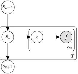
[image:4.612.111.241.55.179.2]st−1
Figure 1: Plate notation for DLVM (T: total number of time instants).
wherePt(f)is the probability of frequencyf att,P(f|zi)is
a multinomial distribution (similar to that used PLCA [1]), and the coefficients of the mixture are Pt(zi),i∈ {1,2, ....K}.
Our model assumes that the latent bases P(f|zk) are the
same at all time instants. The bases are source-specific and are viewed as the spectral signatures of the sources. On the other hand, the coefficients Pt(zk) vary over time, and they
describe the probability of each latent base at a given time t. Let ntdenote the observation vector at time instant t (the
tthcolumn of the matrixN). Let us now define a state,s t, of
the observation vector nt as follows
st= [Pt(z1), Pt(z2), ..., Pt(zk)]T
= [st(1), st(2), ..., st(K)]T (3)
In general, static LVMs assume that the mixture coefficients
Pt(zk) (hence, the states st) are independent at all time
instants. However, this assumption limits the effectiveness of the LVMs for modeling time varying signals. Our model addresses this limitation by imposing a Markovian dependence between states using a Dirichlet distribution. Note that the support of the states st of dimension K lies on a K−1
di-mensional simplex. The Dirichlet distribution has been widely used as a distribution on simplex and is the conjugate of multinomial. Also, it belongs to the exponential family and has finite dimensional sufficient statistics [3]. These properties lead to intuitive and efficient parameter estimation discussed in Section IV. The proposed model is described below in detail.
A. DLVM
To model the temporal dependence between states, we propose a Dirichlet distribution with time-varying parameters
P(st|st−1,D) = Dir(αt−1Dst−1+1)
where αt= X
f
Nf t (4)
P(s1) = Dir(1)
where, ‘Dir’ denotes the Dirichlet distribution,αtdenotes the
total number of observations at timet,1is an all-one vector,
andDis a temporal dependence matrix defined as follows
D=
d11 d12 . . . d1K
d21 d22 d23 . . . d2K
..
. ... ... . .. ...
dK1 dK2 dK3 . . . dKK
(5)
where, dij ∈ R+ denotes the temporal dependence between
states at two consecutive time instants for the ith and jth
latent basis. A higher value of dij indicates higher temporal
dependence.
The Dirichlet-multinomial conjugacy allows us to have an intuitive understanding of the parameters of the Dirich-let distribution as pseudo observations. Let us define the pseudo observation for the kth basis at time t as m
tk =
αt−1(Dst−1)(k). Therefore (4) can be rewritten as follows
P(st|st−1,D) = Γ(P
k(mtk+ 1)) Q
kΓ(mtk+ 1)) Y
k
st(k)mtk (6)
where, Γ(x) is the Gamma function. Note that the hyperpa-rameters of the Dirichlet distribution are dynamic. Hence, we refer to it as thedynamic Dirichlet distributionin the rest of this paper.
Let ζt be a αt-dimensional vector, where ζt(l) ∈
{z1, z2, ...zK}contains the active latent basis of thelthcount
of the observation vector nt. According to our model, the
generative process of Nis as follows:
• Samplest∼Dir(αt−1Dst−1+1)
• Sample frequencyf,αt times as follows:
– Choose a latent basisζt(l)∼Mult(st)
– Choose a frequencyf ∼Mult(P(f|ζt(l))).
• Repeat the above processT times.
where,T is the total number of time instants, ‘Mult’ denotes the multinomial distribution. We observe that each sample is a realization of a mixture multinomial (for simplicity, we use the notation of the categorical distribution, also the conjugate of Dirichlet, for the multinomial distribution. It is a common practice [3], and has no effect on parameter estimation). We as-sume that the counts in an observation vector at a time instant are independent and identically distributed. Fig. 1 presents a graphical model for the proposed generative process.
The proposed dynamic Dirichlet distribution prior has the following appealing properties which provides an intuitive understanding:
• The generative process (with mixture multinomial as the likelihood) allows us to view the spectrogram at timetas an observed count data overKbases. Static models such as PLCA uses this observation data to estimate the states at each time instant. The dynamic Dirichlet prior allows us to havemtkextra pseudo observations for each basisk
at time instantt, which is the result of the multinomial-Dirichlet conjugacy [30]. This observation will become clear in (16) later. A higher number of observations at previous time instant (αt−1) or higher value of temporal
dependence (djk) leads to a higher count of pseudo
• The mode of the distribution lies at the normalized pseudo observations
max
k (st(k)|st−1) =
mtk P
kmtk
• The variance of each entry of the vector st can be
obtained from the properties of the Dirichlet distribution [30]
V ar(st(k)|st−1)∝
1 (P
kmtk+K)2( P
kmtk+K+ 1)
which decreases as the total number of observations at previous time instant i.e.,αt−1increases. A higher value
of αt−1 indicates that more prior information (more
pseudo observation) is available. This trend in variance is expected because the distribution should have less variance when there is more prior information from previous time instant.
The proposed DLVM can be interpreted as a three-level hierarchical Bayesian model similar to the LDA [3]. In our model, P(f|z) is the source level parameter (sampled once for each source), while st is the time level (sampled once
at every time instant), and zk andf are the frequency level
(sampled once per frequency) parameters.
B. PLCA as a special case of DLVM
The relationship between the proposed DLVM and the well known PLCA model is particularly interesting. When the temporal dependence matrixDis reduced to a zero matrix, the distribution in (4) becomes a symmetric Dirichlet distribution
Dir(1). Note that the symmetric Dirichlet distributionDir(1)
is nothing but a uniform distribution, and thus, the formulation in (4) is equivalent to the static PLCA. This can also be intuitively understood as the fact that in the absence of prior information, there is no prior preference of any state over the others. Writing the parameters of dynamic Dirichlet as:
αt−1Dst−1+1=αt−1D(st−1+1) + (I−αt−1D)1
where,Iis an identity matrix. The first term contains the prior information from the previous time instant. The second term contains the content of uniform distribution. Whenαt−1Dis
an identity matrix, the prior has no component of uniform distribution and is completely decided by the past information. The amount of past information is controlled by the total number of observed count at previous time instant (αt−1). C. Bidirectional DLVM
We assumed that st depends only on the immediate past
state st−1. This degree of dependence can be relaxed, and
more states can be included to account for longer temporal dependence. For example, a natural extension would be to include the temporal dependence both in the past and in the future states.
Let us denote the forward dependence (i.e., dependence on the past states) matrices asD+1,D+2, ...D+l and the backward dependence (i.e., dependence on the future states) matrices as
D−1,D−2, ...D−l , where the model orderl is a positive integer.
f z
αt
st
st+1
T
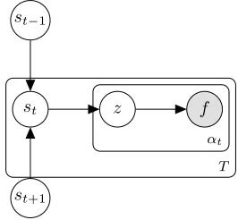
[image:5.612.370.503.56.179.2]st−1
Figure 2: Plate notation for bi-DLVM (order =1).
D+l denotes the temporal dependence between st on st−l
while D−l denotes the temporal dependence between st on st+l. The dynamic Dirichlet distribution in this case takes the
following form
P(st|st−l, ...,st+l,D+1,D
−
1, ...,D + l ,D
−
l ) =
Dir( l X
j=1
αt−jD+jst−j+αt+jD−jst+j+1)
(7)
where,ldenotes the maximum degree of temporal dependence in the model. To keep the equations simple, we considerl= 1. Let us denoteD+1 andD−1 as the forward and the backward dependence matrices. The single order bi-DLVM (referred to as the bi-DLVM in rest of the paper) is given by
P(st|st−1,st+1,D+1,D
−
1) =
Dir(αt−1D+1st−1+αt+1D−1st+1+1)
(8)
The corresponding graphical model is presented in Fig. 2. Note that the proposed bi-DLVM (see (8)) reduces to the earlier proposed DLVM forD1−= 0.
IV. PARAMETERESTIMATION
In this section, we describe the parameter estimation steps for the proposed DLVM. We derive an EM algorithm for the same.
Let us denote the state matrix S = [s1, ...st, ...sT], β=
{P(f|z),D1+,D1−}, Λ = {β,S} and ζ = [ζ1, ..ζt, .., ζT].
Let us denote the (i, j)th element of D1+ andD1− as d+ij
andd−ij respectively.
The joint probability of the observed and the latent variables given the parameterβ is as follows
P(S, ζ,N|β) =P(S|β)P(N, ζ|S, β) =
=Y
t
P(st|st−1) αt
Y
l=1
(P(f|ζt(l))Pt(ζt(l)) !
(9)
This is obtained using Markovian dependence between states at different time instants, and the assumption that given
The likelihood of the observed spectral data matrix N is obtained by marginalizingζ andS
P(N|β) = (10) Y
t
Z
st
P(st|st−1) Y
f X
k
P(f|zk)st(k) !Nf t
dst
Our aim is to estimate Λˆ so as to maximize the above marginalized likelihood (see 10). EM is a common approach to maximize log-likelihood in presence of latent variables. It consists of two iterative updates: i) an expectation (E) step, where the posterior distribution of the latent variables is computed; and ii) a maximization (M) step, where the expected log-likelihood is maximized with respect to the posterior distribution. The posterior distribution of latent variables is given by
P(S, ζ|N, β) = P(S, ζ,N|β)
P(N|β) (11)
However, the denominator (see (10)) is computationally in-tractable [3] [31]. Sampling techniques, such as MCMC, or approximate inference techniques, such as variational Bayes inference can be employed to address the issue. However, for simplicity, we perform a MAP estimate of the states instead of a fully Bayesian inference. Therefore, we maximize the following
ˆ
Λ ={β,ˆ Sˆ}= argmax Λ
P(N,S|β) (12)
= argmax Λ
Y
t
P(st|st−1) Y
f X
k
P(f|zk)st(k) !Nf t
The steps in our EM algorithm are described below.
A. Expectation step
The posterior distribution of zis given by
Pt(zk|f) =
Pt(zk)P(f|zk) P
kPt(zk)P(f|zk)
(13)
B. Maximization step
We intend to maximize the following MAP function
LM AP = E
Pt(z|f)
log(P(N,S, ζ|β))
= E
Pt(z|f)
log(P(N, ζ|S, β)) + log(P(S|β)) (14)
s.t., X
f
P(f|zk) = 1, X
k
st(k) = 1, 0< d+ij, d
−
ij ∀ i, j
The objective functionLM AP is concave with respect to each
of the parameters (S, P(f|z),D1+,D1−) provided others
are fixed. 1.
1Our proof of concavity: https://tinyurl.com/yxm9gqy7
1) Update of P(f|z): Maximizing the above constrained expected log-likelihood in (14) with respect toP(f|zk)yields
the following
P(f|zk) = P
tNf tPt(zk|f) P
f P
tNf tPt(zk|f)
(15)
Note that this update for the latent basisP(f|zk)is the same
as that for PLCA [4].
2) Update of S: Let us now define pseudo observation from the previous and the next time instants asm+tk andm−tk
for a basis kas follows
m+tk=αt−1(D1+st−1)(k)
m−tk=αt+1(D1−st+1)(k)
We perform a sequential update for the states S in forward direction starting from the first time instant. While estimating
st,st−1appears inside the Gamma function which has already
been estimated. Therefore, the proposed updates are in closed form unlike that in other models based on estimating parame-ters of Dirichlet (e.g., Latent Dirichlet allocation, Hierarchical Dirichlet process).
MaximizingLM AP with respect tost(k)while keepingD+1
andD−1 fixed yields
st(k) = P
fNf tPt(zk|f) +m + tk+m
−
tk P
k( P
fNf tPt(zk|f) +m+tk+m
−
tk)
(16)
We see that the updates of the states contain additional terms (m+tk, m−tk) as compared to those in PLCA. We call them as pseudo observation for each basis k. This update is similar to the updates of the states in Kalman filtering [24].
3) Updates of D+1, D−1: The update of D+1 andD−1 is dependent on scaling factorγ. However, we ignore its effects and justify the assumption by empirical results.
MaximizingLM AP with respect toD+1 (keeping SandD
−
1
fixed) does not have any closed form solution.
D+1 = argmax
D+1
X
t
log Γ(X k
(m+tk+m−tk+ 1))− X
k
log Γ(m+tk+m−tk+ 1) +X k
m+tk(k) log(st(k))
s.t., 0< d+ij, ∀ i, j. (17) However, the maximizing function is concave since Dirichlet distribution belongs to the exponential family of distributions 1. Therefore, the function has a unique maxima, which can be obtained via gradient ascent
∂LM AP
∂d+ik =
X
t
αt−1st−1(i)
ψ X
j
(m+tj+m−tj+ 1) −ψ(m+tk+m−tk+ 1) + log(st(k)
(18)
where, ψ is the digamma function. D−1 is updated similarly. However, we find the above equations to be computationally expensive. Therefore, we restrict the dependence matrices (D+1
andSare independent of the scaling factorγ. Therefore, the proposed algorithm is applicable to both count and non-count data, and we may replaceNbyX(refer (1)) in all the update equations.
V. DLVMAS ADYNAMICNMF
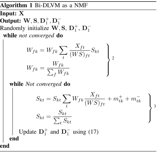
In this section, we show that the proposed DLVM can be viewed as a dynamic version of NMF. It has been shown in the literature that an LVM can be interpreted as an NMF for specific cost functions [32]. The update equations for PLCA and NMF with Kullback–Leibler (KL) divergence have been shown to be the same [32]. The NMF interpretation of PLCA leads to very compact and fast update equations. Similarly, we can interpret the DLVM (dynamic counterpart of PLCA) as a dynamic version of NMF. Below, we present the update equations for our bi-DLVM as a dynamic version of NMF. The updates of DLVM as a dynamic version of NMF can be obtained by settingD1− to a zero matrix.
Algorithm 1 Bi-DLVM as a NMF
Input:X
Output: W,S,D+1,D−1
Randomly initializeW,S,D+1,D−1
whilenot converged do
Wf k =Wf k X
t
Xf t (W S)f t
Skt
Wf k =
Wf k P
fWf k
2
while Not convergeddo
Skt=Skt X
t
Wf k
Xf t (W S)f t
+m+tk+m−tk
Skt=
Skt P
tSkt
3
Update D+1 andD−1 using (17) end
end
DLVM learns the latent bases and the states for an observed data matrix via the following factorization
Pt(f) = K X
k=1
Pt(zk)P(f|zk)
Multiplying both sides of the above equation by αt, we
rewrite the equation in matrix-vector form as nt = Wstαt,
where,Wis a matrix whose columns are latent basesP(f|z). Concatenating observation vectornt for all time instants, we
can write the observed data matrixXas,
XF×T =WF×KSK×TGT×T =WF×KHK×T
where, W is the basis matrix, S is the state matrix, G
(normalization matrix) is a diagonal matrix with αt as the 2From (13) and (15)
3From (13) and (16)
diagonal elements, and the subscripts denote dimensions of the matrices. The (f, k)th element in W is denoted as W
f k
and the (k, t)th element in Sis denoted as S
kt. It is evident
that all matrices (X,W,S,G) are non-negative. Therefore, we can view the proposed DLVM as a dynamic version of NMF with iterative updates forW,SandD (see Algorithm 1). In Algorithm 1, the outer loop corresponds to the EM iteration, while the inner loop corresponds to the block-wise update of variables in the maximization step of the EM algorithm.
4
VI. APPLICATIONS TOAUDIOPROCESSING
In this section, we demonstrate the usefulness of the pro-posed DLVM model and its variant for three audio processing tasks: (i) speaker source separation, (ii) denoising, and (iii) bandwidth expansion. To this end, we also propose a new algorithm for dynamic source separation.
A. Source separation
Source separation is a long standing problem in signal processing, which aims to recover the constituent source signals from a given mixture signal. It has wide applications in speaker recognition, speech enhancement, music editing and audio information retrieval [33], [34]. In this section, we develop an algorithm for dynamic source separation using the bases learned from bidirectional DLVM with dependence matrices as D+1 andD−1.
We assume that the given mixture signal is a linear com-bination of a known number of speaker signals. The spectral distribution of a mixture signal is given by
Pt(f) = X
a
Pt(a)Pt(f|a) = X
a
Pt(a) X
zk∈za
Pt(zk|a)P(f|zk)
(19)
where,Pt(a)denotes the apriori probability of theathsource.
The parameters associated with theathsource are denoted as Λa ={Sa, βa}.
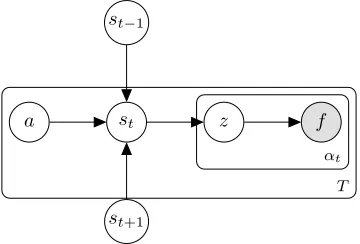
[image:7.612.49.311.284.532.2]The graphical model of the mixture signal is presented in Fig. 3. Our objective is to separate the constituent sources from a mixture signal. Following the supervised paradigm, we learn the parameters βa for all a from the training data. These parameters are later used to separate the sources in the separation stage.
Let us consider a mixture spectrogram X. The parameters
Pt(a)andPt(z|a)are learned from Xvia an EM algorithm.
In the expectation step, we estimate the posterior distribution and the expected number of total observation, αat, for each
source. In the maximization step, we maximize the expected log-likelihood
LM AP = E
Pt(z,a|f)
log(P(N,S, ζ, a|β)) (20) where,β,Sandζcontains latent variables and parameters for all the sources. The steps in the EM algorithm are as follows
f z
αt
st
a
st+1
T
[image:8.612.85.265.56.178.2]st−1
Figure 3: Plate notation of the mixture signal modeled using bi-DLVM, adenotes an audio source.
1) Expectation step:
Pt(a, zk|f) =
Pt(a)Pt(zk|a)Pa(f|zk) P
a0Pt(a0)Pzk∈za
0Pt(zk|a0)Pa0(f|zk)
(21)
αat =
X
f
Xf t
Pt(a) (22)
2) Maximization step:
ma+tk =αat−1X
j
da+kjPt−1(zj|a)
matk−=αat+1X
j
dakj−Pt+1(zj|a)
Pt(zk|a) =
P
fXf tPt(a, zk|f) +ma+tk +m a−
tk
P zk∈za
P
fXf tPt(zk, a|f) +ma+tk +m a−
tk
(23)
Pt(a) = P
zk∈za
P
fXf tPt(a, zk|f) P
a0
P zk∈za
P
fXf tPt(a0, zk|f)
After the above EM algorithm converges, the reconstructed spectral vector for each source is obtained as the expected value ofXf tover all sources as follows.
Pt(f|a) = X
zi∈za
Pt(zi|a)Pa(f|zi) ˆ
Xf t(a) =E(Xf t(a)) =
Pt(a)Pt(f|a)Xf t P
a0Pt(a0)Pt(f|a0)
Finally, the phase of the mixture signal is combined with the reconstructed magnitude spectrogram (Xˆf t(a)) to recover each
source signal [1].
B. Denoising
We consider a speech denoising scenario, where the speech signal is degraded by an additive noise. We follow a speaker dependent approach i.e., we assume that the identity of the speaker is known. We also assume that the noise type (e.g., babble, factory) is known and training data for each noise type is available. This assumption is practical in many scenarios
where classification techniques can be employed for detecting the noise type and speaker identity [17]. We consider the noise and the speaker’s data as two distinct sources, and learn the latent bases separately for the them. We learn the parameters for each speaker and each noise type from the training data. The speech is separated from the noise using the source separation algorithm described in Section VI-A.
C. Bandwidth expansion
In this section, we develop an algorithm for bandwidth expansion for a band limited signal that utilizes the latent bases learned using DLVM. Bandwidth expansion of a signal may be required in different scenarios, e.g., for signals that are sampled at a low sampling rate, high frequency components may be lost, or, for signals incurring distortion in some frequency bands, or, when the signal acquisition system is incapable of capturing frequencies beyond a particular range. We address the problem of bandwidth expansion of a narrow band (0−4 KHz) speech signal. Using the bases learned by our model, we predict the higher frequency components (4−8
KHz) from a given narrow band speech signal. Let us denote the observed frequencies asfo∈ {0-4KHz}and unobserved
frequencies asfu∈ {4-8KHz}. First, we learn the parameters
for a speech signal (β) for all frequencies from the training data. We use these parameters to estimate states and the total number of draws (αt) using only the observed frequencies.
The following equation is used iteratively to estimate st(k)
from the band limited signal X
st(k) = P
foXf tPt(zk|f) +m
+ tk+m
−
tk
P k
P
foXf tPt(zk|f) +m
+ tk+m
−
tk
Once the above iterative updates converge, we estimate αt
using only the observed frequencies. Finally, the unobserved frequencies are predicted.
Pt(fu) = K X
k=1
Pt(zk)P(fu|zk)
αt= P
foXf t
P
foPt(f)
Xfut=αtPt(fu)
The phase values at the unobserved frequencies are esti-mated separately. Since, phase also contains negative values, our algorithm is not appropriate for phase prediction. We therefore assume that the phase of the unobserved frequencies
Φu are a linear transformation of phase of the observed
frequencies Φo i.e., Φu = AΦo [35]. The transformation
matrix Ais learned from the phase of the training data Φtr.
The least square estimate ofA is given by A= Φtr u(Φtro)†,
where(·)† denotes pseudoinverse. Finally, the phase and the magnitude spectrogram are multiplied, and converted to time domain signal using STFT.
VII. EXPERIMENTALVALIDATION
three audio processing tasks described in the previous section. We also compare the performance of the proposed model with several other existing methods.
A. Experimental setup
We use the TIMIT database [18] and the signal processing information base (SPIB) [19] to carry out our experiments. The TIMIT database contains broadBand recordings of630 speak-ers sampled at16KHz, each speaker reading ten phonetically rich sentences. The SPIB database contains noise data of 15
different noise types acquired with a sampling frequency of
19.98KHz, an analog to digital converter (A/D) with16bits, an anti-aliasing filter, and without a pre-emphasis stage.
All audio signals were downsampled to 16 KHz. The spectrograms are obtained by performing STFT using a
64ms window with 16ms overlap. The resulting magnitude spectrograms are then processed and analyzed further. The phase spectrograms are analyzed separately, agnostic to the algorithm, using standard methods [4]. We have used 250
iterations for the outer loop, and 10 iterations for the inner loop in DLVM (Algorithm 1). The dependence matrices (D1+,D1−) were fixed to 0for first 50iterations.
Evaluation metrics: In order to evaluate the source
separation and denoising performance, we use the following evaluation metrics (i) signal to noise ratio improvement (SNRI) [36], (ii) source to distortion ratio (SDR), (iii) source to interference ratio (SIR), and (iv) source to artifact ratio (SAR) [34] [37]. The later three provide perceptual evaluation of the source separation results. We have used the BSS-EVAL TOOLBOX [38] for evaluation.
Let X and φ represent the magnitude and the phase of a mixture signal. Let Xo andXrrepresent the original and
re-constructed signal spectrogram from the mixture respectively. The SNR improvement (SNRI) of a speaker is calculated by incorporating the phase information and by comparing the improvement in terms of SNR. Define a gain function for a spectrogram Y
g(Y) = 10 log10
P f,t(X
o)2 f t
P
f,t|(Xo)f texp(jφf t)−Yf texp(jφf t)| 2
SNRI is defined as SNRI=g(Xr)−g(X).
In order to evaluate bandwidth expansion, we use generalized KL divergence (GKL) and Itakuro-Saito (IS) divergence [36], [39]. Both the metrics have been widely used as cost functions in NMF, and are appropriate for computing the distance between two data distributions which are the scaled versions of any probability distributions [36], [39].
Comparison: The performances of DLVM and bi-DLVM
are compared with those of four existing methods: PLCA [1], PLCA with dynamic filtering [29], PLCA with dynamic smoothing [29] and dynamic NMF with exponential prior [17]. These methods were chosen because they all offer probabilistic interpretations and were developed primarily for source separation. For PLCA with dynamic filtering and smoothing, we report the best results obtained after
0 1 2 3
Fr
eq
ue
nc
y(
Hz
)
0 4000 8000
(a)
0 1 2 3
Fr
eq
ue
nc
y(
Hz
)
0 4000 8000
(b)
Time(sec)
0 1 2 3
Fr
eq
ue
nc
y
(H
z)
0 4000 8000
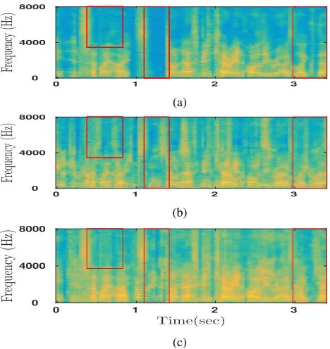
[image:9.612.313.547.56.304.2](c)
Figure 4: Sample result for speaker source separation: (a) orig-inal source, (b) recovered source using PLCA, (c) recovered source using DLVM.
SNRI SDR SIR SAR
dB
0 2 4 6 8
10 PLCA Dynamic filt Dynamic smooth Dynamic NMF DLVM Bi-DLVM
Figure 5: Performance comparison for speaker source separa-tion in terms of four evaluasepara-tion metrics.
hyperparameter tuning in our experiments. No hyperparameter tuning is required for dynamic NMF and proposed methods.
B. Speaker source separation
We follow an experimental setup similar to that described in the literature of source separation using PLCA and its variants [40], [7]. We have used ∼ 25 seconds of speech (8 to9 sentences) from20 speakers (10male, 10 female) in the TIMIT database. To model each speaker (source), the first ∼17seconds of the speech is used. The remaining5seconds was used to create190synthetic mixtures by adding the speech from two speakers. The speech signals were normalized to zero mean and unit variance prior to addition. We learn K = 30
latent bases in each case. Finally the spectral vector for each source is reconstructed using steps outlined in section VI-A.
[image:9.612.320.551.362.476.2]Model Order (l)
0 0.5 1 1.5 2 2.5 3
SNRI (dB)
5.5 6 6.5
[image:10.612.64.282.61.162.2]PLCA Dynamic Filt Dynamic Smooth DLVM Bi-DLVM Dynamic NMF
Figure 6: Source separation performance with varying model order.
results on source separation, Fig. 4a shows the original spec-trogram while Fig. 4b and Fig. 4c present the reconstructed spectrograms of the given source recovered (from a mixture) using PLCA and DLVM respectively. Notice that DLVM recovers a smoother or better spectrogram (areas exhibiting significant differences are highlighted).
Fig. 5 shows the average values across 190 test cases for all methods. As seen in Fig. 5, DLVM and bi-DLVM perform better than or comparable to the existing methods in terms of all metrics. DLVM outperforms dynamic NMF (with exponential prior) by 0.65 dB in terms of SNRI,0.52 dB in SDR,0.99dB in SIR, and0.12dB in SAR. The improvement in terms of SAR implies that the artifacts introduced by DLVM are less compared to other models. Usually, there is a trade-off between removing noise (measured by SDR and SNRI) and introducing artifacts (measured by SAR). The simpler dynamic models ([29]), while improving SDR often introduce more artifacts, which lead to a degraded SAR. However, DLVM and its variant show simultaneous improvement in terms of both SDR and SAR. This indicates an overall better modeling ability of DLVM, which leads to better source separation.
Fig. 6 shows the variation of output SNRI with the model orderl. Note thatl= 0corresponds to the static PLCA. In our experiments, we observe thatl= 1is sufficient to capture the temporal dependencies efficiently for dynamic and bi-DLVMs. No further improvement in output SNRI is observed forl >1. The inability of better performance forl >1can be attributed to the fact that the model only performs temporal smoothing on the coefficient matrix, and longer-term temporal smoothing does not contribute in this case due to the non-stationary nature of the data. We believe that DLVM withl= 1(which has low complexity) should be preferred over other models if MAP estimation is to be performed.
C. Denoising
We choose six noise types (babble, factory, white, pink, cockpit and military vehicle noise) for this experiments. This noise is added (one at a time) to the speech data of the 20
speakers used in the speaker source separation experiments. Both the noise and the speech are first normalized to have zero mean and unit variance. The noisy mixtures are obtained by adding the noise to each speaker signal. The amount of training data and number of latent bases (K) for each speaker and noise are identical to those used in Section VII-B.
Time (sec)
0 1 2
F
re
qu
en
cy
(H
z)
0 4000 8000
Time (sec)
0 1 2
Time (sec)
[image:10.612.320.554.61.147.2]0 1 2
Figure 7: Sample denoising result: (left) original source (left), (center) source recovered by PLCA , and (right) DLVM at
[image:10.612.312.567.220.375.2]6dB SNR.
Table I: Performance comparison for denoising
Babble Factory White Pink Cockpit Military Avg
Average SDR
PLCA [1] 5.92 4.01 5.75 3.55 3.97 4.26 4.58
Dynamic filt [29] 5.89 3.87 5.68 3.31 3.81 4.28 4.47
Dynamic smooth [29] 5.95 3.22 5.69 2.75 3.61 3.96 4.19
Dynamic NMF [17] 5.86 5.42 5.44 3.77 4.09 3.65 4.71 DLVM 6.08 5.99 5.40 5.49 4.56 4.50 5.34
Bi-DLVM 5.71 4.56 4.59 5.63 4.59 4.77 4.98
Average SAR
PLCA [1] 6.69 8.20 8.93 7.98 8.27 8.44 8.08
Dynamic filt [29] 6.44 7.94 8.67 7.32 8.01 8.53 7.81
Dynamic smooth [29] 5.65 6.93 8.45 6.25 7.70 7.94 7.15
Dynamic NMF [17] 8.30 9.09 9.09 8.27 8.27 8.30 8.55 DLVM 7.22 9.38 9.51 8.94 9.18 8.78 8.83
Bi-DLVM 7.20 9.27 8.70 8.69 8.84 9.04 8.62
Fig. 7 presents a sample (qualitative) denoising result, where the source was corrupted with pink noise at 6 dB SNR. Observe that DLVM yields better reconstruction compared to PLCA - which loses almost all structures at higher frequencies. The performance of DLVM (averaged over 20 mixtures at
6 dB SNR) is presented in Table I along with results from existing methods. DLVM shows an improvement (on average) of0.59dB in terms of SDR and0.28dB in SAR as compared to dynamic NMF. Interestingly, DLVM performs better than all methods for all noise types, except white noise. This can be explained by the fact that white noise is stationary and has no temporal structure, which DLVM attempts to capture. Nevertheless, our model performs better in all those cases where the noise is non-stationary, as it is able to learn the temporal dependencies in the data and the noise. DLVM shows
0.75dB SAR improvement on average for all noise types over PLCA. This observation supports our earlier claim that the proposed model introduces less artifacts as compared to other models.
Fig. 8 shows the denoising performance of the proposed and existing methods at different SNR levels. DLVM (or its variant) outperforms all methods for all noise types except white noise at every input SNR level (as observed earlier).
D. Bandwidth expansion
Input SNR (dB)
0 2 4 6 8
O u tp u t S D R (d B ) 2 3 4 5 6 7
(a) Babble noise
Input SNR (dB)
0 2 4 6 8
O u tp u t S D R (d B ) 0 2 4 6
(b) Factory noise
Input SNR (dB)
0 2 4 6 8
O u tp u t S D R (d B ) 0 2 4 6
(c) White noise
Input SNR (dB)
0 2 4 6 8
O u tp u t S D R (d B ) 0 2 4 6
(d) Pink noise
Input SNR (dB)
0 2 4 6 8
O u tp u t S D R (d B ) 0 2 4 6
(e) Cockpit noise
Input SNR (dB)
0 2 4 6 8
O u tp u t S D R (d B ) 0 2 4 6
(f) Military vehicle noise
[image:11.612.312.548.56.381.2]PLCA Dynamic filt* Dynamic smooth* DLVM Bi-DLVM Dynamic NMF
[image:11.612.48.293.57.467.2]Figure 8: Denoising performance with varying SNR
Table II: Performance comparison for bandwidth expansion in terms of average GKL and IS divergence
Methods GKL IS
PLCA [1] 349.3 482.5
Dynamic filt [29] 289.1 334.0
Dynamic smooth [29] 248.8 2394.9
Dynamic NMF [17] 279.5 297.6 DLVM 237.8 214.7
Bi-DLVM 263.4 338.7
data. Following the earlier works in the literature, the value of
K was chosen to be100for better prediction [35]. All other experimental details for the training stage are identical to those described in Section VII-B.
Fig. 9 shows a sample bandwidth expansion result using PLCA and DLVM. The latter yields a smoother spectrum compared to PLCA (difference areas highlighted). Recall that we utilize DLVM only to reconstruct the magnitude spectrogram. The phase spectrogram was predicted separately using least square solution [35]. For quantitative comparison
0 1 2 3 4 5
Fr
eq
ue
nc
y
(Hz
)
0 2000 4000 6000 8000 (a)0 1 2 3 4 5
Fr
eq
ue
nc
y
(Hz
)
0 2000 4000 6000 8000 (b)0 1 2 3 4 5
Fr
eq
ue
nc
y
(Hz
)
0 2000 4000 6000 8000 (c) Time(sec)0 1 2 3 4 5
Fr
eq
ue
nc
y
(Hz
)
0 2000 4000 6000 8000 (d)Figure 9: Sample result for bandwidth expansion: (a) bandlim-ited signal, (b) original signal, (c) bandwidth expansion using PLCA, and (d) bandwidth expansion using DLVM.
of different algorithms for bandwidth expansion we used GKL divergence and IS divergence as metrics. Results averaged over
20speakers are shown in Table II.
Table II shows that DLVM-based solution has the least KL divergence and IS divergence with respect to the ground truth. This shows that DLVM has better prediction ability, which is due to the better modeling capability of DLVM. Also, we observe that the DLVM outperforms bi-DLVM. This can be attributed due to the i)fact that the model only performs temporal smoothing on the coefficient matrix, and longer-term temporal smoothing does not contribute in this case due to the non-stationary nature of the data, ii)The dependencies in our data are mostly unidirectional.
E. Compactness of the representation
Along with the various results, we would also like to high-light an important observation regarding the state estimates (st) obtained using DLVM and its variant. Fig. 10 shows
[image:11.612.96.248.533.606.2]0 1 2 3
S
ta
te
5 10 15 20 25 30
(a)
0 1 2 3
S
ta
te
5 10 15 20 25 30
(b)
Time(sec)
0 1 2 3
St
at
e
5 10 15 20 25 30
0
0.2
0.4
0.6
0.8
[image:12.612.55.302.57.281.2]1
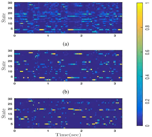
Figure 10: Compactness of representation indicated by state activation in (a) PLCA, (b) DLVM, and (c) bi-DLVM.
Table III: Sparsity of the state matrixS
Methods `0 `0.1 Entropy
PLCA [1] 21.07 1.94×10¹² 2.24
Dynamic filt [29] 20.2 1.16×10¹² 2.14
Dynamic smooth [29] 17.74 5.02×10¹¹ 1.94
Dynamic NMF [17] 19.75 2.64×10¹² 2.10
DLVM 5.59 1.64×10⁹ 0.82
Bi-DLVM 5.58 2.13×10⁹ 0.81
[41]. To quantify this sparsity, we use Shannon’s entropy,`0.1
and `0 norm [7], [42]. We compute the `0 norm after hard
thresholding the values at0.001. Table III shows the sparsity of the state matrix for different methods. The`0norm shows that
the average number of active latent bases is the smallest (5.58) in the bidirectional case. The results show that the proposed model naturally learns more compact representation, as we have not used any sparsity prior explicitly in the model. The Dirichlet prior induces sparsity only when the values of each of its parameters are less than 1. However, the parameters in the proposed dynamic Dirichlet prior are defined to be greater than 1, which promotes a dense distribution [3]. This leads us to hypothesize that the sparsity observed in the proposed model is due to its ability to learn better representation. In contrast, exponential prior in dynamic NMF ([17]) has an average of19.7active bases. Also in Fig., 10, we observe that the posterior estimates of states (although, we have imposed smooth prior on states,) are able to capture sharp transition better than PLCA.
VIII. CONCLUSION
We proposed a dynamic latent variable model, called the Dirichlet latent variable model, for learning latent bases from time varying non-negative data. To capture the temporal struc-tures in data efficiently, we introduced a dynamic Dirichlet
prior - a Dirichlet distribution with dynamic parameters. A major contribution of this work is to introduce the dynamic Dirichlet prior for non-negative data. We showed that the expected log-likelihood function is concave and can be solved by standard convex optimization methods. This property arises because of (a) Dirichlet-multinomial conjugacy and (b) Dirichlet and multinomial are member of exponential family distributions. The proposed DLVM can be interpreted and implemented as a dynamic version of NMF. We also showed that the popular PLCA model is a special case of DLVM. An EM algorithm was developed for the parameter estimation of DLVM. Through extensive experiments, we demonstrated that DLVM outperforms several existing methods for three appli-cations: speaker source separation, denoising and bandwidth expansion. Unlike existing dynamic models (which contain annealing hyperparameter), DLVM does not require any free parameters to be set by the user, other than the number of bases to be learned. The updates of latent bases and states is independent of scaling factor. Therefore, DLVM can handle non-count data as well. Although the current work in this paper involves modeling magnitude spectra of audio signals (non-count data), DLVM is suitable for modeling other types of non-negative data, such as word count data which appears widely in natural language processing. We also showed that the dynamic Dirichlet prior leads to sparse states (which is well proven to be better representation). Also, we observe that the posterior estimates of states can have sharp transition and has been captured by our model efficiently.
Future work will be directed towards developing faster updates for dependence matrices (D1+ and D1− in this
paper), and a fully Bayesian inference algorithm instead of a MAP estimate of states.
ACKNOWLEDGEMENT
The authors would like to thank Prof. Ketan Rajawat, IIT Kanpur for various technical discussions related to this work.
REFERENCES
[1] P. Smaragdis, B. Raj, and M. Shashanka, “A probabilistic latent vari-able model for acoustic modeling,” Advances in models for acoustic
processing, NIPS, vol. 148, pp. 8–1, 2006.
[2] T. Hofmann, “Probabilistic latent semantic indexing,” inProceedings of the 22nd annual international ACM SIGIR conference on Research and
development in information retrieval. ACM, 1999, pp. 50–57.
[3] D. M. Blei, A. Y. Ng, and M. I. Jordan, “Latent dirichlet allocation,”
Journal of machine Learning research, vol. 3, no. Jan, pp. 993–1022,
2003.
[4] B. Raj, M. V. Shashanka, and P. Smaragdia, “Latent dirichlet decompo-sition for single channel speaker separation,” inAcoustics, Speech and Signal Processing, ICASSP Proceedings. IEEE International Conference on, vol. 5. IEEE, 2006, pp. V–V.
[5] A. Hadgu and Y. Qu, “A biomedical application of latent class models with random effects,”Journal of the Royal Statistical Society: Series C
(Applied Statistics), vol. 47, no. 4, pp. 603–616, 1998.
[6] D. D. Lee and H. S. Seung, “Learning the parts of objects by non-negative matrix factorization,”Nature, vol. 401, no. 6755, pp. 788–791, 1999.
[7] M. Shashanka. (1999) Results and demos. [Online]. Available: http://cns.bu.edu/∼mvss/courses/speechseg/
[image:12.612.65.281.339.421.2][9] Z. Chen and A. Cichocki, “Nonnegative matrix factorization with tem-poral smoothness and/or spatial decorrelation constraints,”Laboratory
for Advanced Brain Signal Processing, RIKEN, Tech. Rep, vol. 68, 2005.
[10] N. Mohammadiha, P. Smaragdis, and A. Leijon, “Supervised and unsu-pervised speech enhancement using nonnegative matrix factorization,”
IEEE Transactions on Audio, Speech, and Language Processing, vol. 21,
no. 10, pp. 2140–2151, 2013.
[11] S. Hiroya, “Non-negative temporal decomposition of speech parameters by multiplicative update rules,”IEEE Transactions on Audio, Speech,
and Language Processing, vol. 21, no. 10, pp. 2108–2117, 2013.
[12] P. Smaragdis, “Convolutive speech bases and their application to su-pervised speech separation,”IEEE Transactions on Audio, Speech, and
Language Processing, vol. 15, no. 1, pp. 1–12, 2007.
[13] W. Wang, A. Cichocki, and J. A. Chambers, “A multiplicative algorithm for convolutive non-negative matrix factorization based on squared euclidean distance,”IEEE Transactions on Signal Processing, vol. 57, no. 7, pp. 2858–2864, 2009.
[14] D. Kounades-Bastian, L. Girin, X. Alameda-Pineda, S. Gannot, and R. Horaud, “A variational em algorithm for the separation of time-varying convolutive audio mixtures,”IEEE/ACM Transactions on Audio,
Speech, and Language Processing, vol. 24, no. 8, pp. 1408–1423, 2016.
[15] G. J. Mysore, P. Smaragdis, and B. Raj, “Non-negative hidden markov modeling of audio with application to source separation,” in
Interna-tional Conference on Latent Variable Analysis and Signal Separation.
Springer, 2010, pp. 140–148.
[16] A. Kumar, T. Guha, and P. Ghosh, “A dynamic latent variable model for source separation,” inAcoustics, Speech and Signal Processing, 2018.
ICASSP 2018 Proceedings. 2018 IEEE International Conference on.
[17] N. Mohammadiha, P. Smaragdis, G. Panahandeh, and S. Doclo, “A state-space approach to dynamic nonnegative matrix factorization,”IEEE
Transactions on Signal Processing, vol. 63, no. 4, pp. 949–959, 2015.
[18] J. S. Garofolo, L. F. Lamel, W. M. Fisher, J. G. Fiscus, and D. S. Pallett, “DARPA TIMIT acoustic-phonetic continous speech corpus cd-rom. nist speech disc 1-1.1,”NASA STI/Recon technical report n, vol. 93, 1993. [19] U. K. Speech Research Unit (SRU) at Institute for Perception-TNO,
Netherlands. Signal processing information base (SPIB). [Online]. Available: http://spib.linse.ufsc.br/noise.html
[20] C. F´evotte, N. Bertin, and J.-L. Durrieu, “Nonnegative matrix factor-ization with the itakura-saito divergence: With application to music analysis,”Neural computation, vol. 21, no. 3, pp. 793–830, 2009. [21] T. Virtanen, “Monaural sound source separation by nonnegative matrix
factorization with temporal continuity and sparseness criteria,” IEEE
transactions on audio, speech, and language processing, vol. 15, no. 3,
pp. 1066–1074, 2007.
[22] P. Smaragdis and B. Raj, “Shift-invariant probabilistic latent component analysis, tech report,” 2007.
[23] P. Smaragdis, C. Fevotte, G. J. Mysore, N. Mohammadiha, and M. Hoff-man, “Static and dynamic source separation using nonnegative factor-izations: A unified view,”IEEE Signal Processing Magazine, vol. 31, no. 3, pp. 66–75, 2014.
[24] M. S. Grewal, “Kalman filtering,” in International Encyclopedia of
Statistical Science. Springer, 2011, pp. 705–708.
[25] S. J. Julier and J. J. LaViola, “On kalman filtering with nonlinear equality constraints,”IEEE Transactions on Signal Processing, vol. 55, no. 6, pp. 2774–2784, 2007.
[26] D. Simon, “Kalman filtering with state constraints: a survey of linear and nonlinear algorithms,”IET Control Theory & Applications, vol. 4, no. 8, pp. 1303–1318, 2010.
[27] A. Carmi, P. Gurfil, and D. Kanevsky, “Methods for sparse signal recovery using kalman filtering with embedded pseudo-measurement norms and quasi-norms,” IEEE Transactions on Signal Processing, vol. 58, no. 4, pp. 2405–2409, 2010.
[28] C. F´evotte, J. Le Roux, and J. R. Hershey, “Non-negative dynamical system with application to speech and audio,” inAcoustics, Speech and
Signal Processing (ICASSP), 2013 IEEE International Conference on.
IEEE, 2013, pp. 3158–3162.
[29] N. Mohammadiha, P. Smaragdis, and A. Leijon, “Prediction based filtering and smoothing to exploit temporal dependencies in nmf,”
in Acoustics, Speech and Signal Processing (ICASSP), International
Conference on. IEEE, 2013, pp. 873–877.
[30] K. W. Ng, G.-L. Tian, and M.-L. Tang,Dirichlet and related
distribu-tions: Theory, methods and applications. John Wiley & Sons, 2011,
vol. 888.
[31] J. M. Dickey, “Multiple hypergeometric functions: Probabilistic in-terpretations and statistical uses,”Journal of the American Statistical
Association, vol. 78, no. 383, pp. 628–637, 1983.
[32] M. Shashanka, B. Raj, and P. Smaragdis, “Probabilistic latent variable models as nonnegative factorizations,”Computational intelligence and
neuroscience, 2008.
[33] X. Yu, D. Hu, and J. Xu,Blind source separation: theory and
applica-tions. John Wiley & Sons, 2013.
[34] E. Vincent, N. Bertin, R. Gribonval, and F. Bimbot, “From blind to guided audio source separation: How models and side information can improve the separation of sound,”IEEE Signal Processing Magazine, vol. 31, no. 3, pp. 107–115, 2014.
[35] B. Raj, R. Singh, M. Shashanka, and P. Smaragdis, “Bandwidth ex-pansionwith a p´olya urn model,” in Acoustics, Speech and Signal
Processing, ICASSP . IEEE International Conference on, vol. 4. IEEE,
2007, pp. IV–597.
[36] M. Shashanka, “Latent variable framework for modeling and separating single-channel acoustic sources,” Ph.D. dissertation, BOSTON UNI-VERSITY Boston, 2007.
[37] E. Vincent, R. Gribonval, and C. F´evotte, “Performance measurement in blind audio source separation,”IEEE transactions on audio, speech,
and language processing, vol. 14, no. 4, pp. 1462–1469, 2006.
[38] C. F´evotte, R. Gribonval, and E. Vincent, “BSS EVAL toolbox user guide–revision 2.0,” 2005.
[39] D. FitzGerald, M. Cranitch, and E. Coyle, “On the use of the beta divergence for musical source separation,” 2009.
[40] B. Raj and P. Smaragdis, “Latent variable decomposition of spectro-grams for single channel speaker separation,” in IEEE Workshop on
Applications of Signal Processing to Audio and Acoustics. IEEE, 2005,
pp. 17–20.
[41] B. A. Olshausen and D. J. Field, “Natural image statistics and efficient coding,”Network: computation in neural systems, vol. 7, no. 2, pp. 333– 339, 1996.
[42] R. G. Baraniuk, “Compressive sensing [lecture notes],” IEEE signal
processing magazine, vol. 24, no. 4, pp. 118–121, 2007.
Anurendra Kumarcompleted his B.tech-M.tech in Electrical Engineering from IIT Kanpur in 2017. His interest is in developing robust, scalable and efficient machine learning algorithms for real world applications. Currently, he is a co-founder in a start-up project, where he leads the team focused on designing mathematical techniques for futuristic financial services and risk management.
Tanaya Guha is an Assistant Professor in the department of Computer Science, University of War-wick, UK. Prior to joining WarWar-wick, she worked in IIT Kanpur as an assistant professor, and in Univer-sity of Southern California as a postdoctoral research fellow. She has received her PhD in Electrical and Computer Engineering from the University of British Columbia (UBC), Vancouver. She was a recipient of Mensa Canada Woodhams memorial scholarship, Google Anita Borg scholarship and Amazon Grace Hopper celebration scholarship. Her current research interests include multimodal signal processing and multimedia analysis.