Collaborative Filtering in the News Domain with Explicit and Implicit Feedback

(1)

Collaborative Filtering in the News

Domain with Explicit and Implicit

Feedback

Dag Einar Monsen

Patrick Heia Romstad

Master of Science in Computer Science Supervisor: Jon Atle Gulla, IDI

Department of Computer and Information Science Submission date: June 2014

(2)

(3)

Abstract

In online recommender systems, we use computerized algorithms to present arti-cles targeted at the preferences of each individual user. One such technique, called collaborative filtering, works by selecting articles that is preferred by users with preferences similar to those of the target user. There are different ways to deter-mine a users preference. A common practice is to ask for it, for instance by offering the user to provide a rating from one to five. Users are, however, often reluctant to provide such information. From a usability perspective, it is better to look at their behaviour, or implicit feedback, and use that to infer their preferences.

The main goal of this thesis is to determine whether we can use such implicit feedback in order to improve the accuracy a collaborative filtering method. We have implemented and tested a number of standard machine learning algorithms for mapping implicit feedback to explicit ratings. These algorithms are applied to a news data set consisting of user interactions collected while reading and rating news articles. After the mapping techniques have inferred possible new ratings, the next step is to generate recommendations, which is done with a matrix factorization algorithm. To measure the effect of adding implicit feedback to the recommendations we calculate the root mean square error (RMSE).

We have developed a fast and scalable collaborative filtering component and inte-grated it with a news aggregation service called SmartMedia. The component uses a combination of nearest neighbor search on articles with more than 30% correla-tion and a time threshold of 20 seconds to infer ratings based on user interaccorrela-tions collected. We show that these methods improve the RMSE by 5.14% compared to using only ratings users have given.

Our work shows that utilizing implicit feedback can improve recommendation ac-curacy in the news domain. The techniques we have developed require less explicit rating to be given from users in order to create good recommendations. Thus we believe that the next generation of recommender systems will be less dependent on explicit rating while still being able to provide high quality recommendations.

(4)

(5)

Sammendrag

I nettbaserte anbefalingssystemer kan vi bruke algoritmer for ˚a presentere en sam-ling artikler tilpasset hver individuelle bruker. ´En slik teknikk, kalt collaborative filtering, fungerer ved ˚a anbefale artikler foretrukket av brukere med samme prefer-anser som m˚albrukeren. Det er ulike m˚ater ˚a avgjøre slike preferanser. En vanlig praksis er ˚a spørre om det, for eksempel ved ˚a tilby brukeren ˚a gi en karakter fra en til fem. Brukere er imidlertidig ofte motvillige til ˚a oppgi slik informasjon. Fra et brukbarhetsperspektiv er det bedre ˚a se p˚a deres interaksjoner, eller implisitte brukerdata, og bruke det til ˚a gi anbefalinger.

Hovedm˚alet med denne masteroppgaven er ˚a avgjøre om vi kan bruke slik implisitt brukerdata for ˚a forbedre nøyaktigheten til et anbefalingssystem. Vi har imple-mentert og testet ulike maskinlæringsalgoritmer som oversetter implisitt bruk-erdata til eksplisitte karakterer. Alle algoritmene har blitt testet p˚a et nyhets-datasett som best˚ar av brukerinteraksjoner som har blitt innsamlet mens bruk-erne har lest og gitt karakterer til nyhetsartiklene. Etter at brukerdata har blitt oversatt til karakterer, er det neste steget ˚a lage anbefalinger ved hjelp av matrise-faktorisering. For ˚a m˚ale effekten av ˚a utnytte brukerdata til ˚a lage anbefalinger, beregner vi rotmiddelkvadratavviket (RMSE).

Vi har utviklet en kjapp og skalerbar anbefalingskomponent, og integrert den med en nyhetsinnsamler kalt SmartMedia. Komponenten bruker en kombinasjon av nærmeste nabosøk p˚a nyhetsartikler med mer enn 30% korrelasjon og en tidsterskel p˚a 20 sekunder for ˚a inferere nye karakterer basert p˚a innsamlet brukerdata. Vi viser at disse metodene forbedrer RMSE med 5.14% sammenliknet med metoder som kun utnytter eksplisitte karakterer.

Arbeidet v˚art viser at implisitt brukerdata kan forbedre anbefalingsnøyaktigheten i nyhetsdomenet. Teknikkene vi har utviklet krever færre karakterer fra brukere for ˚a kunne gi gode anbefalinger. Vi tror derfor at neste generasjons anbefal-ingssystemer vil være mindre avhengige av karakterer for ˚a kunne gi anbefalinger av høy kvalitet.

(6)

(7)

Preface

This master’s thesis is the culmination of our work, carried out during the 10th

semester of our Master of Computer Science degree at the Norwegian University of Science and Technology, NTNU.

We wish to thank our supervisor Professor Dr. Jon Atle Gulla and co-supervisor ¨

Ozlem ¨Ozg¨obek at the Departement of Computer and Information Science, Nor-wegian University of Science and Technology for helpful guidance throughout the project.

Trondheim, June 5, 2014 - Dag Einar Monsen and Patrick Heia Romstad

(8)

(9)

List of Figures

2.1 iPhone application . . . 8

2.2 Overall architecture of the SmartMedia news application . . . 9

2.3 Different recommendation factors . . . 9

3.1 Simple example of collaborative filtering . . . 16

3.2 Example of grouping articles by content-based filtering . . . 20

5.1 Users and movies in the latent space . . . 29

6.1 Tucker decomposition of a three-dimensional tensor . . . 36

6.2 CANDECOMP/PARAFAC decomposition of a three-dimensional tensor . . . 36

7.1 Examples of different values for the correlation coefficient . . . 38

7.2 Example of bins with equal size . . . 40

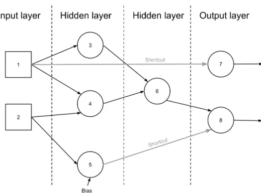
7.3 A multilayer perceptron with two hidden layers . . . 43

7.4 Example of a SVM hyperplane . . . 44

7.5 A hierarchical clustering over animal descriptions . . . 47

9.1 The SmartMedia recommender integration . . . 60

10.1 The steps in preprocessor . . . 66

11.1 Time on page versus ratings before and after sampling the YOW data set: (a) before and (b) after . . . 75

11.2 RMSE of best performing techniques compared to baseline . . . 78

11.3 Rating frequency in data set . . . 79

11.4 Time on page versus ratings . . . 79

11.5 Naive Bayes configuration plotted at different classify threshold with baseline estimate border . . . 89

(14)

(15)

Part I

Introduction

(16)

(17)

Chapter 1 Introduction

In this chapter we introduce our thesis. In Section 1.1 we explain our motivation to work with recommender systems in the news domain. In Section 1.2 we discuss what problems we have investigated in our thesis and in Section 1.3 we explain how we approached these problems. Then we present a summary of our findings in Section 1.4 and finally, in Section 1.5 we outline the structure of our thesis.

1.1 Background and Motivation

With the advent of the Internet, the media industry has found itself going through a radical transformation. In the scope of the last two decades, traditional printed newspapers have seen their readership decline as a result of competition by on-line publishing. Using mobile devices with Internet access, people can read news articles in the moment they are published – from anywhere in the world. This transformation naturally implicates many challenges for newspaper companies. It does, however, also involve many opportunities for those who are able to adapt. A printed newspaper is usually composed of articles selected to satisfy as many readers as possible. One can target a certain market segment, but targeting a single user is not feasible in print. In the electronic medium, on the other hand, a newspaper company can look at the reading patterns of every single user, and make an estimate of which articles they will find to be interesting. That is the domain of news recommender systems. There are many different ways to make such an estimate. A common method, known as collaborative filtering, works by the assumption that a user will prefer articles that are preferred by similar users,

(18)

4 Chapter 1 Introduction

where users are assumed to be similar if they have expressed similar preferences to items in the past. Users often express these preferences as a numeric rating from 1-5, or on a different scale. Users are, however, often reluctant to provide such explicit feedback, and we cannot expect users to rate every article they read. In addition, we can look at how users interact with a system. How much time do they spend reading an article? Do they share it with their friends? This kind of information does not require an explicit action from the user, it is merely collected as he or she uses the system. In this master’s thesis, we explore how this implicit feedback can be used to improve the accuracy of a recommender.

1.2 Problem Statement

News recommendation involves a set of unique challenges, especially the lack of explicit feedback to many articles. In our work, we explore ways to make use of implicit feedback available to improve the accuracy of a collaborative filtering algorithm, and how to integrate these methods to a real system. Formally, we attempt to answer the following research questions:

R1: How can we use implicit feedback to improve news recommendation accuracy in collaborative filtering?

Specifically, we want to investigate how we can decrease the Root Mean Squared Error (RMSE) of the recommender system using implicit feedback. The decrease in RMSE can then be compared to other research papers that consider implicit feedback as a method to increase recommendation accuracy.

R2: How do different techniques for including implicit feedback com-pare?

Implicit feedback in this thesis consists of user-article interactions that can be collected without any overhead to the user, while explicit feedback are ratings given explicitly by the user after reading an article. The techniques we compare utilize implicit feedback that only exists in the data set given, and we will therefore not utilize information about the users from other sources. Consequently, the techniques convert implicit feedback to explicit feedback through mapping in such a way that we can run matrix factorization recommender algorithms with the resulting explicit feedback.

(19)

Chapter 1 Introduction 5

R3: How can a collaborative filtering component be integrated with the SmartMedia news aggregator?

As the SmartMedia news aggregator utilizes a variety of filtering methods, we need to implement our component as a standalone application that supports a standard interface. The SmartMedia news aggregator can then control the priority between different filters to give an optimal set of articles.

1.3 Approach

To find solutions for these problems, we need a deep understanding of the problem space and the domain in focus. Based on an extensive knowledge search, we implement a number of standard machine learning algorithms for mapping from implicit to explicit ratings. These are applied to a news data set consisting of user interactions collected while reading and rating news articles.

The evaluations are done with the prospect of integrating a recommendation com-ponent to the SmartMedia news aggregator. With this integration we can present novel and interesting articles to users based on their reading habits.

1.4 Results

The evaluations demonstrated that given the right mapping technique, mapping implicit feedback to explicit feedback can improve accuracy of recommendations in the news domain. In addition, the mapping technique that improved accuracy the most, is a combination of using nearest neighbor search with one neighbor and a time threshold of 20 seconds, which had a 5.14% improvement. Our results also show mapping techniques that looks for global patterns in the dataset, as opposed to patterns for each item, is detrimental for recommendation accuracy.

Further, we developed a stand-alone collaborative filtering component that inte-grates with the SmartMedia application. The component consists of a combina-tion of a mapping technique and a parallel matrix factorizacombina-tion algorithm based on stochastic gradient descent. It is scalable and fast, computing recommendations in less than 150 milliseconds. The components implements a standard REST API, and can easily be replaced by improved components in the future.

(20)

6 Chapter 1 Introduction

1.5 Thesis Structure

Chapter 2 - The SmartMedia Project: A quick overview of the NTNU Smart-Media Project and how we contribute to it.

Chapter 3 - Recommender Systems: An introduction to news recommenda-tions and collaborative filtering.

Chapter 4 - Feedback: A thorough discussion about feedback and the differ-ences between explicit and implicit feedback.

Chapter 5 - Matrix Factorization: Describes matrix factorization and how it can be used as a collaborative filtering component.

Chapter 6 - Tensor Factorization: Describes tensor factorization and how it can be used as a collaborative filtering component.

Chapter 7 - Mapping Techniques: Explanation of different techniques that maps implicit feedback to explicit ratings.

Chapter 8 - Related Work: A survey of related work in recommender systems.

Chapter 9 - Implementation: Implementation details of the recommender and how the recommender is integrated to the SmartMedia application.

Chapter 10 - News Recommendation in the SmartMedia Application:

Explains how feedback is represented, preprocessed and used to generate recom-mendations.

Chapter 11 - Evaluation of Mapping Techniques: Describes the evaluation setup and the results from our evaluations.

Chapter 12 - Integrational Issues: A discussion of the integration to Smart-Media in terms of modifiability and scalability.

Chapter 13 - Discussion and Conclusions: A final discussion including con-clusions and suggestions for further work.

(21)

Chapter 2 The SmartMedia Project

In this chapter we give a brief overview of the NTNU SmartMedia project. In Section 2.1, we outline the project background, in Section 2.2 we show the archi-tecture of the news aggregator and in Section 2.3 we show how user profiling is done. Finally, in Section 2.4 we outline our contribution to the project.

2.1 Project Background

The NTNU SmartMedia project was established in 2012 in close collaboration with the Scandinavian media industry. The team is led by Prof. Jon Atle Gulla, and is divided into different research areas. Nafiseh Shabib is working on group recommendations. Özlem Özgöbek is working on data collection and semantics. Dag Einar Monsen and Patrick Heia Romstad are working on the collaborative filtering part of the recommender system. Dr. Jon Espen Ingvaldsen is working on content filtering and the underlying news index. Martin Akre Midstund and Marius Krakeli have been working on geospatial filtering. P˚al-Christian Salvesen and Lars Smør˚as Høysæter are working on sentiment analysis of news articles. Kent Robin Haugen has made a client application for the iOS platform, and Amir Ghoreshi and Neberd Salimi are working on a web-based client application.

The main goal of the SmartMedia project is to create a mobile application that efficiently recommends news articles to users and is easy to use. An early version of the iPhone application is presented in Figure 2.1. Technologies involved in making

(22)

8 Chapter 2 The SmartMedia Project

Figure 2.1: iPhone application

this application are big data architectures, information retrieval, semantics, text analytics and sentiment analysis as well as various frameworks.

2.2 System Architecture

The news recommender system is structured as a traditional client-server archi-tecture, as shown in Figure 2.2. The server side will aggregate news articles daily from all (89) major online newspapers in Norway by parsing their RSS feeds for all metadata, including the ingress. The aggregator proceeds by scraping the website of each newspaper for the full article content. All of these articles are written in Norwegian, and are provided in a semi-structured format. In some articles, we are able to obtain certain features like topic or category from the RSS feed. We also apply entity recognition to each article. Using entity recognition, we are able to extract locations, names of people and other interesting features which can then be used to support a number of recommendation techniques, including information

(23)

Chapter 2 The SmartMedia Project 9

Figure 2.2: Overall architecture of the SmartMedia news application

filtering, geospatial filtering and content filtering. The recommendation process is discussed further in [1] and a diagram of this process is presented in Figure 2.3.

(24)

10 Chapter 2 The SmartMedia Project

The client application is designed using web technology, simplifying a cross-platform deployment. The application is independent of each publisher, and we plan to al-low voluntary sign-ups, thus our knowledge about each client is limited to the data we collect. We allow each user to rate an article by a 1-5 star rating. We also take note of certain user interactions, which we elaborate further on in Section 4.2.

2.3 User Profiling

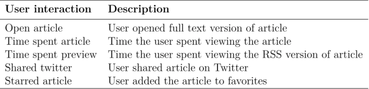
User profiling is important for the SmartMedia application in order to do individual recommendations for each user. A user profile is constructed for a chosen time interval, and if there already exists a user profile for this mobile device, the profiles are combined in such a way that the new profile is weighted more than the old one[2]. This way of constructing user profiles enables the recommender system to (i) do recommendations to new unregistered users since it constructs a user profile for each session, and (ii) give improved recommendations to registered users by combining the constructed user profiles. Therefore, the second (ii) step becomes crucial to build long-term user profiles. Examples of user interactions collected by the SmartMedia applications are shown in Table 2.1.

The user profile consists of two vectors P =< ~C, ~K >[2]. C~ is a category vector where each news category is given a weight that indicates how important this category is for the user. K~ is a content vector that weights key phrases and entities that the user might find interesting. Examples of C~ and K~ vectors are shown in Equation 2.1 and 2.2.

~

C =<(”N EW S”,98.0),(”T ECH”,50.0),(”SP ORT S”,15.4),(”ST Y LE”,2.5)>

(2.1)

~

K =<(”iP hone”,20.0),(”T yson”,5.0),(”LG”,3.4),(”Abra”,0.41), . . . > (2.2)

While the C~ vector is limited to the number of categories, the K~ vector grows as the user reads news articles. Since only the highest weighted terms are relevant for the recommendation stage, the less important terms can be removed to ensure the

(25)

Chapter 2 The SmartMedia Project 11

Table 2.1: Examples of user interactions used to construct user profiles

User interaction Description

Open article User opened full text version of article Time spent article Time the user spent viewing the article

Time spent preview Time the user spent viewing the RSS version of article Shared twitter User shared article on Twitter

Starred article User added the article to favorites

vector do not become unnecessary large. More information about SmartMedia’s approach to user profiling is further described in [2].

These user profiles are currently not used by the collaborative filtering component, but resembles the user and item vectors created in the matrix factorization stage. The differences between these vectors and the user profiles are that the user and item vectors created by the collaborative filtering component comprises of the latent factors found, and do not have labels that describe them. It is therefore challenging to incorporate the user vectors created by our component with the user profiles created by the SmartMedia application.

2.4 Our Contribution

Our part in the NTNU SmartMedia Project is to implement an efficient and accu-rate collaborative filtering algorithm. To do so, we intend to incorpoaccu-rate implicit feedback as well as explicit feedback in the recommender engine and analyze the results of this implementation.

(26)

(27)

Part II

Background

(28)

(29)

Chapter 3 Recommender Systems

In this chapter we introduce the theory behind recommender systems and their applications. In Section 3.1 we outline the motivation behind recommender sys-tems. In Section 3.2 we describe collaborative filtering and in Section 3.3 we reason about news recommendation and what distinguishes it from other domains.

3.1 Introduction

As the internet has become a primary source of information, finding what one is looking for can be a challenge. When looking for a specific piece of information, a user normally uses a search engine like Google or Bing to retrieve a list of re-sults matching their query. A common use case, however, occurs when we are not looking for something specific, but merely something interesting. A simple way of providing such items is to retrieve the most popular items in a catalog. A more personalized approach, on the other hand, can recommend items based on the preferences of each individual user. Schafer et al.[3] argues that personal recommendations will increase sales by converting browsers into buyers, increas-ing cross-sell opportunities, and buildincreas-ing customer loyalty. Linden et al.[4] also saw increased sales and customer retention at the online retailer Amazon.com by showing a list of similar items below each item. We normally divide recommender systems into two categories. In a content-based approach, users are often encour-aged to state their topics of interest. In a news domain, this can for example be sports and politics. Items are then defined with a set of features, where a set of topics would be a feature of a news article. A recommender system would then

(30)

16 Chapter 3 Recommender Systems

Figure 3.1: Simple example of collaborative filtering

be able to recommend articles by calculating the similarities between the users expressed interests and each item, thus returning the most similar ones.

Another method of providing recommendations is to look for similar users. If a user B has shown to have similar preferences to a user A, one might recommend a book to user B that user A finds interesting, and user B has not read yet, as shown by the dotted line in Figure 3.1. This method of providing recommendations is called collaborative filtering. A more thorough introduction to collaborative filtering is given in the next section.

In our work, we have implemented a collaborative filtering component and inte-grated it with the SmartMedia application, allowing users to read news selected to their personal preferences.

3.2 Collaborative Filtering

Collaborative filtering recommends items to a user by looking at similar users and recommend items that they have expressed an interest in. The basic form of collaborative filtering takes in a matrix of user-item ratings as input and produces two types of output: (i) a numerical prediction of the degree a user will like or dislike an item and (ii) a list of n recommended items.

Collaborative filtering can be divided in two categories: memory-based and model-based. Given a matrix of user-item ratings, memory-based collaborative filter-ing uses the matrix on each query to generate new item recommendations to the user. The most common method of memory-based collaborative filtering is

(31)

Chapter 3 Recommender Systems 17

neighborhood-based collaborative filtering with item-based or user-based top-n recommendations.

Collaborative filtering methods face certain challenges depending on the particular domain. In Section 3.3 we discuss the challenges unique to the news domain. There are, however, a range of challenges faced by collaborative filtering methods that are common to most domains. Data sparsity: data sets often consist of many more user-item combinations than there are interactions between these. The user-item matrix of the 100M netflix data set contained 17770 movies and 480189 users, resulting in a density of roughly 1.17%[5]. Such sparse data sets means that the algorithms have to make predictions based on very little information. This challenge is related to the cold start problem, which refers to what occurs when new users or items enter the system. These additions do not have any feedback as new users have not rated any items, and new items have not been rated. This is a problem, because the collaborative filtering methods need feedback in order to provide recommendations. Collaborative filtering methods also face a challenge when the scale of the system increases. As new users and items are added to the system, the user-item matrix thus increases. This means that the memory-based methods have to iterate over an increasing number of rows and columns in the user-item matrix. This will eventually lead to performance problems and new recommendations cannot be computed fast enough.

This problem led researchers to look at different methods for computing recom-mendations. Using machine learning techniques, an intermediate representation of the user-item matrix could be computed, and then used to make recommenda-tions with less computational effort. This intermediate representation is called a model and we call these methods model-based. Model-based methods using ma-trix factorization has been shown to scale to hundreds of millions of entries in the user-item matrix[6, 7]. Matrix Factorization works by modeling ratings as a sparse matrix indexed by user ID and item ID, and then factorizing this matrix into a product of matrices of much lower dimensions. This smaller representation can then be used to estimate ratings very efficiently. We explore matrix factorization further in Chapter 5.

A challenge with matrix factorization surfaces when we want to include implicit data in the model. By allowing the matrix to contain more than a single feedback value in each cell, we effectively have what is called a tensor of three dimensions, as a matrix is merely what we call a two-dimensional tensor. For clarity, a single

(32)

dimensional tensor of numbers is simply a vector. Thus, tensor factorization, as opposed to matrix factorization, deals with the factorization of a generalized tensor of N dimensions. Tensor factorization does, unfortunately, also involve a set of challenges. We discuss these challenges further, as well as methods to do tensor factorization for providing recommendations in Chapter 6.

An alternative to tensor factorization works by combining the feedback values prior to building a model. When we have both implicit and explicit feedback available, we can try to find patterns between them. From these patterns, we might be able to estimate the explicit feedback, which means that we no longer have to collect an explicit feedback value from a user – we can rely solely on his or her actions. If we are able to infer explicit feedback from implicit feedback, we might be able to improve the accuracy of a model computed using matrix factorization. This has been the main focus of our thesis, and we discuss these mapping techniques further in Chapter 7.

3.3 News Recommendation

Following the same approach as other recommender systems, the purpose of a news recommender system is to find and present news articles that a user might find interesting. Using the definition presented in [2], this can be formulated as

s:U ×A→V (3.1)

where s is the utility function, U the set of users, A the set of news articles and

V is an ordered set of values representing the rating or preference of a user for an article. Then the purpose of a recommender system is to recommend an articlea0

that maximizes the utility function for the user.

a0 = arg max

a∈A

s(u, a) (3.2)

There are many important factors to consider when recommending news articles due to the complexity of the news domain compared to other domains e.g. books, movies and songs. The recommender system must be robust and tackle changes in the news domain. Robustness is needed according to Gulla et al. [2] since news

(33)

Chapter 3 Recommender Systems 19

articles are unstructured and require a thorough analysis, and unlimited reach of news lead to changes in terminologies and topics over time.

Factors closer to the part of generating recommendations are location and freshness of the news articles. Location is used to give users recommended articles that are either close to their physical location or news about their hometown. Freshness is just as important — we need to present the latest news to users. The approach we make in SmartMedia are geospatial and temporal filtering, as presented in Figure 2.3.

The key challenge in the domain of news recommendation is item churn[6]. Item churn can be mitigated with memory-based methods, but as mentioned in the previous section, memory-based methods become infeasible when we have millions of users and items. For this reason, we use a model-based approach. However, since news articles are added and deleted at a high frequency, it becomes difficult to keep the model up to date.

Other challenges mentioned in [2] are cold start problems due to new and unread news and the ability to recommend new articles to a user in topics the user have never read (serendipity). Cold start problems in news recommendation is more difficult to handle than in more stable item set, such as movies, since news articles are continuously added. Serendipity is important in order to give the user more varied set of news articles.

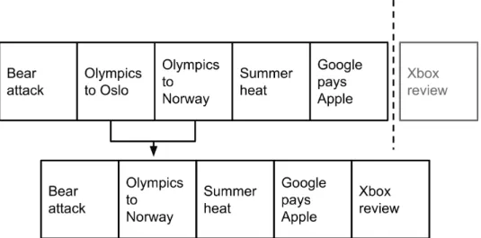
Additionally, a problem occurs when the system aggregates news from many dif-ferent sources. In this case, we might have multiple articles on the same subject. A collaborative filtering system does not necessarily see this similarity, and may thus recommend several articles on the same subject to a user. In this case, we can use a content-based filtering system to discover these similarities and group the articles written on the same subject. This is illustrated in Figure 3.2, where we recommend five articles.

(34)

(35)

Chapter 4 Feedback

Feedback from users is essential for recommender systems, but collecting sufficient user information is a challenge. User information can be collected in two ways: explicit and implicit. In sections 4.1 and 4.2 we outline these two kinds of feedback, respectively.

4.1 Explicit Feedback

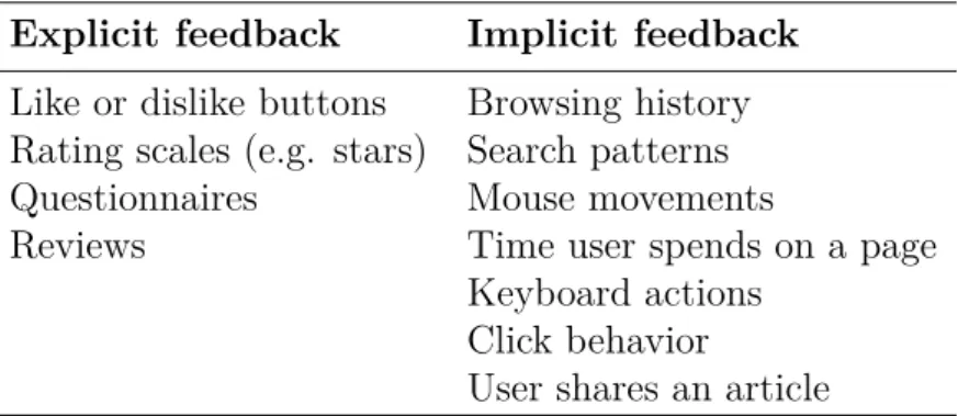
Explicit feedback is so named because the user provides it explicitly. This means that it depends on users willingness to provide such feedback. A five star ratings scale is an example of explicit ratings given by users; other examples are listed in Table 4.1. Explicit feedback is generally considered as more reliable than implicit feedback, but it also suffers from noise or inconsistencies[8]. Amatriain et al. provide an in-depth analysis of user rating noise in recommender systems in [9]. Some of their main findings were: (i) extreme ratings are more consistent than mild opinions and (ii) users are more consistent when items with similar ratings are grouped together. Knowing that extreme ratings are more consistent enables us to give higher weight to articles with extreme values when we are mapping implicit feedback to explicit feedback.

Another issue with explicit feedback in news recommendation is, according to Thurman[10], that users are often reluctant to give explicit feedback on news articles that can be used to construct and maintain user profiles. Therefore, a rec-ommender system should not impose any requirements to the user to give explicit

(36)

22 Chapter 4 Feedback

feedback, and the final SmartMedia application will only use implicit feedback to generate recommendations. However, explicit feedback will be collected to build the data set used in this master’s thesis. How this feedback is collected and used to create user profiles should then be described, encouraging the test users to leave explicit feedback.

Furthermore, even though explicit feedback contains noise, it is generally accepted that it is more reliable than implicit feedback in most situations[9]. It will therefore be used as the true preference for articles in the data set used in our evaluation. This enables us to transform implicit feedback to an explicit rating through various techniques explained in Chapter 7.

Table 4.1: Common types of explicit and implicit feedback

Explicit feedback Implicit feedback

Like or dislike buttons Browsing history Rating scales (e.g. stars) Search patterns Questionnaires Mouse movements

Reviews Time user spends on a page Keyboard actions

Click behavior

User shares an article

4.2 Implicit Feedback

Implicit feedback relies on collecting user information by analyzing user actions or content that users interact with. Examples of user actions are time spent read-ing an article, click behavior and time spent on movread-ing the mouse/cursor. More examples are listed in Table 4.1. The main advantages of collecting implicit feed-back are: (i) users do not have to actively engage to provide useful information to the recommender system and (ii) implicit feedback can be combined with explicit ratings to obtain a more accurate representation of user interests[11].

Implicit feedback has several challenges. Hu et al. [12] list four prime character-istics: (i) No negative feedback: When observing user actions we can infer which items users probably like, but we can not assume users dislike items they have not interacted with. (ii) Implicit feedback is noisy: We can only guess users preferences for items. (iii) Implicit feedback uses confidence, that is, how much confidence do

(37)

Chapter 4 Feedback 23

we have about users preference and (iv) implicit feedback recommender systems requires appropriate evaluation methods. With implicit feedback we have to no way of clearly measuring what is a successful prediction, as opposed to explicit ratings where we can measure the success of a prediction with a numeric score like RMSE.

However, if we have enough implicit ratings we can assume that low feedback is negative feedback [13], contradicting the first characteristic of Hu et al. But it requires that the items can be grouped into instances that more feedback means higher preference. One example is TV-shows, where more feedback usually means that the user like the show and watches it every week. However, in the news domain this is not the case as users normally read articles only once, leaving this challenge still viable in the news domain.

Further, as we discussed in Section 4.1, explicit feedback is also noisy. Whereas explicit feedback noise mostly refers to the users preferences changing over time, implicit feedback noise refers to the error the recommender system has when trying to interpret the actions of a user.

In addition, given enough explicit ratings and implicit feedback, an appropriate mapping between explicit and implicit feedback is possible as shown in the news domain by [14, 15] and in the music domain in [13]. The main advantage of mapping instead of interpreting user actions is that we can have a higher confidence in our mapping if the correlation is high. We also have a clear metric for evaluating our results, since we can work on explicit ratings when evaluating the recommender system, but use implicit feedback to improve or add explicit ratings.

(38)

(39)

Chapter 5 Matrix Factorization

This chapter introduces matrix factorization as a technique to generate recom-mendations. Section 5.1 gives a motivation for use and a brief intro to matrix factorization. Then, singular value decomposition is described in Section 5.2. Stochastic gradient descent and alternating least squares are described in Section 5.3 and Section 5.4. At the end we discuss the tradeoffs between methods in Section 5.5.

5.1 Introduction

As we mention in Section 3.2, memory-based collaborative filtering systems met challenges with performance as data sets scaled into millions of users and items. This lead researchers and the industry to look at different ways to handle the scalability issue. As ratings could be expressed as a matrix indexed by users and items, matrix factorization could be a solution. By factorizing the user-item matrix into components of matrices in a much smaller dimension, one could approximate the missing values of the original user-item matrix. The low-dimension matrices in the model would then represent so called latent factors where each user and each item would have their own set of latent factors. Hence, matrix factorization is also sometimes referred to as Latent Semantic Indexing (LSI), or Latent Semantic Analysis (LSA). The latent, or hidden factors represent patterns found in the original user-item matrix. For example, in the domain of movie recommendations, the first cell in the latent factor vector of a movie could represent to which degree the movie contains elements of romance. The first cell in the latent factor vector

(40)

26 Chapter 5 Matrix Factorization

of a user would then represent to which degree that user prefers romantic movies. When computing the estimated rating of that user to that movie, the latent factor vectors are multiplied, and thus if the latent properties of romance of both vectors are high, it directly translates to a high rating. The reason the factors are called latent is that we do not know what each factor represent. In some cases it could be something obscure like the amount of red colored houses appearing in the movie, or something incomprehensible to humans.

Matrix factorization involves a potential challenge when the data set is contin-uously changing. In situations where we have repeated additions and deletions, the model needs to be rebuilt at certain intervals to correctly reflect the data set. If the intervals are not often enough the quality of the recommendations can de-cline, and if they are too narrow the build time might become a computational bottleneck in the system, ultimately leading to lower user satisfaction.

Formally, matrix factorization decomposes two or more matrices such that when multiplied they are returned to the original matrix as shown in Equations 5.1 and 5.2, where M is the original matrix and U and V the matrices that will result in

M when multiplied. M U V      11 12 5 22 24 10 13 11 5      =      1 2 2 4 3 1      ×   3 2 1 4 5 2   (5.1) M2,1 =U2,1×V1,1+U2,2×V1,2 = 2×3 + 4×4 = 22 (5.2)

In collaborative filtering, matrix factorization divides the user-item matrix in two matrices: the user matrix and the item matrix. Each user is associated with a vector pu ∈Rf and each item with a vector qi ∈Rf, where f denotes the

dimen-sionality of the latent factor space, meaning the number of latent factors. The vectorsqi and pu represents the corresponding interest the user has to the factors

of an item. By calculating the dot product of these vectors, we can approximate the rating given by user u to item i, denoted by ˆrui[16].

ˆ

(41)

Chapter 5 Matrix Factorization 27

5.2 Singular Value Decomposition

Singular value decomposition (SVD) is based on a theorem from linear algebra which states that a rectangular matrix M can be broken down into the product of three matrices - an orthogonal matrixU, a diagonal matrix Σ, and the transpose of the orthogonal matrix V. This is presented in Equation 5.4

M =UΣVT (5.4)

where UT_U ₌ _I_, _VT_V ₌ _I_{. The columns of} _U _{are orthonormal eigenvectors of} M MT _{, the columns of V are orthonormal eigenvectors of}_MT_M_{, and Σ is a}

diag-onal matrix containing the square roots of eigenvalues from U or V in descending order[17].

Table 5.1: Rating matrix for a SVD recommender

Amy Bob Charlie Dina The Matrix 1 3 3 5

E.T. 4 3 5 2

iRobot 1 4 3 5

Hercules 3 5 2 1

The matrix in Table 5.1 consists of four users and four movies, and if we use SVD, it will be decomposed into quadratic 4×4 matrices, U, VT and Σ as shown in Equation 5.5. Each row in matrices U and VT _{represents the latent factors for}

(42)

28 Chapter 5 Matrix Factorization U VT         −0.4912 0.5042 0.1050 0.7025 −0.5324 −0.5123 0.6658 −0.1041 −0.5367 0.4641 −0.1787 −0.6816 −0.4327 −0.5177 −0.7168 0.1761                 −0.3500 −0.6063 0.1659 0.6945 −0.5798 −0.1741 −0.7506 −0.2648 −0.5193 −0.1593 0.6327 −0.5519 −0.5213 0.7594 0.0931 0.3780         Σ         12.7314 0 0 0 0 4.3442 0 0 0 0 2.6462 0 0 0 0 0.1913         (5.5)

Then, if we want to use the two most important factors, which are those with the largest singular values, we can choose the two first columns in the decomposed matrices from Equation 5.5. The resulting matrices are presented in Equation 5.6.

U2 V2T Σ2         −0.4912 0.5042 −0.5324 −0.5123 −0.5367 0.4641 −0.4327 −0.5177                 −0.3500 −0.6063 −0.5798 −0.1741 −0.5193 −0.1593 −0.5213 0.7594           12.7314 0 0 4.3442   (5.6)

The matrixU2 present the movies’ and the matrixV2T present the users’ positions

in the latent factor space. Since we chose the two most important factors, the latent factor space is two-dimensional. Figure 5.1 presents how the factor space looks like, where the movies and users are plotted according to their positions given by the decomposed matrices. The latent factor space represents the similarity between the items and users, and when we want to give a recommendation to a new user, lets say Mark, we use his rating vector (the items he has rated) and multiply it with the item matrix and the inverse of the singular value matrix.

(43)

Figure 5.1: Users and movies in the latent space

His position in the latent factor space can be used in recommendations. By using his position in Figure 5.1, we could recommend the movies E.T. and Hercules. The position can also be used to find the closest neighbors that can be used in a neighborhood algorithm, which in his case are Bob and Charlie.

In essence, SVD reduces a high dimensional set of points to lower dimensions that exposes the substructure of the original data. Unfortunately for recommender sys-tems, SVD is undefined when knowledge about the matrix is incomplete. Further, using the only known entries carelessly is highly prone to overfitting. In order to avoid overfitting, research suggests to model directly on the observed ratings while avoiding overfitting through an adequate regularized model[18] as shown in Equation 5.8 min p∗,q∗ X (u,i)∈κ (rui−qiTpu)2+λ(kpuk2+kqik2) (5.8)

where κ is the set of the (u, i) pairs for which rui is known and λ is a constant

(44)

ways to minimize Equation 5.8 and find pu and qu. In the next sections we look

at stochastic gradient descent and alternating least squares.

5.3 Stochastic Gradient Descent

With stochastic gradient descent (SGD)1_{, we minimize the error function in}

Equa-tion 5.8 by an iterative approach. SGD differs from regular gradient descent (GD) since it does not have to iterate through all training examples in order to converge[19]. In some cases it might be less precise than GD, but with large data sets it is superior in terms of performance. The pseudocode for the SGD algorithm is given in Algorithm 1. We pass two parameters to the SGD algorithm; a vector of latent factors ω, which are the parameters of the error function E representing the difference between the actual rating and the estimated rating. The second pa-rameter is the learning rate α, which tells how big steps we want to take towards the minimum. The learning rate depends on the possible values of a rating. A common value is 0.001. Given these two parameters, SGD calculates an approxi-mate minimum by calculating the gradient, or slope of a single training example, and shuffling the samples in each step. With this, the true gradient of E(ω) is approximated.

Data:

ωvector of latent factors

αlearning rate

Result: ωconverged vector of latent factors

while above minimum threshold do

randomly shuffle examples in the training set

for i= 1,2, ...,|ω| do

ωi :=ωi−α∇Ei(ωi)

end end

Algorithm 1: Pseudo code for SGD

(45)

5.4 Alternating Least Squares

Alternating least squares (ALS) works by fixing either pu or qi in order to make

Equation 5.8 quadratic and can therefore be solved optimally. Hence, ALS tech-niques rotate between fixing thequ’s andpu’s. For example, when allqu’s fixed, the

system recomputes thepu’s by solving a least-squares problem, and vica versa[16].

A pseudo code of the algorithm is presented in Algorithm 2.

Data: Empty matrices p and q

Result: Matrices p and q

Initialize matrix q by assigning the average rating for the item as the first row, and small random numbers for the remaining entries;

while rui−qiTpu >error criterion do

Fix q;

Solve p by minimizing the sum of squared errors; Fix p;

Solve q by minimizing the sum of squared errors;

end

Algorithm 2: Pseudo code for ALS

5.5 ALS vs. SGD

In generally, ALS is more expensive than SGD because it has to solve a large number of linear least squares problem. However, according to Makari et al. [20] this computational overhead is acceptable when the rank of the factorization is sufficiently small. Further, big advantages of ALS over SGD is that ALS requires less parameters to be tuned, since SGD makes use of a step size sequence, and easy parallelization since either pu or qu are fixed.

According to experiments shown in [20], SGD is the preferred method when the step size sequence is chosen intelligently. In addition, SGD is less memory-intensive than ALS since ALS needs to store the data matrix twice. Nonetheless, choosing between ALS and SGD on a data set should be decided by evaluation of both algorithms on the relevant data set. In our framework, we have chosen to use an implementation of SGD since the Mahout implementation of ALS was mainly tar-geted towards distributed computing, while the Parallel SGD implementation was

(46)

targeted towards a single multi-core machine2_{. Since we did not have a distributed}

evaluation setup, the SGD implementation performed much better.

(47)

Chapter 6 Tensor Factorization

This chapter will introduce tensor factorization as a framework for generating rec-ommendations. Section 6.1 explains the motivation behind tensor factorization, and how they work. Then we will describe how we can use tensors to do recom-mendations in Section 6.2 and at the end in Section 6.3 we will describe the most popular decompositions of tensors.

6.1 Introduction

As we mention in Section 3.2, we cannot directly express implicit feedback in a two-dimensional user-item matrix. When we add several kinds of feedback to each cell, we effectively have a tensor of three dimensions. These kinds of higher order tensors can also be factorized in order to estimate the missing values. By estimating not only explicit feedback, but all kinds of feedback, we might be able to achieve higher accuracy of recommendations.

Tensor factorization is a general form of matrix factorization. Whereas matrix factorization decomposes a matrix in two or more matrices, tensor factorization decomposes higher order matrices to several smaller matrices. A tensor factoriza-tion of a cubic matrix will result in at least three matrices, one for each axis.

Tensor factorization enables recommender systems to add a contextual element in a tensor, in [21] Thai-Nghe et al. describe a three-dimensional tensor Z of size

U×I×T, where the first and second dimension describe the user and item while the last dimension describe the context, which in their case was time. In the

(48)

34 Chapter 6 Tensor Factorization

following section we describe how to utilize the new dimensions as well as how to decompose the tensor.

6.2 Tensor Factorization in News Recommender

Systems

Having more than two dimensions in recommender systems allows us to make use of contextual information. Examples of contextual information are time, seasonality and location. Thai-Nghe et al.[21] had promising results when they incorporated the time dimension in their predictor of student performance. In their predictor they utilize the time dimension to describe the progression students have on al-gebra in an online tutoring system. Hidashi and Tikk[22] efficiently segmented periodical user behavior in different time bands when they used seasonality as context. A simple example of seasonality is that horror movies are normally seen at night while animation is watched in the afternoon.

Time, seasonality and location are interesting contextual information in the news domain. Time and location are normally incorporated in a news recommender separately besides collaborative filtering, as done in the SmartMedia application. However, as studies shown in [21] and [22], adding time and seasonality as contexts in collaborative filtering improved their recommendations, making it interesting to use these contexts in the news domain as well.

Contextual information can also be feedback as a whole, where both explicit and implicit feedback is stored in the same vector, combining them to feedback. Since implicit feedback is dense, that is, as long as a user has read an article, implicit feedback will always be collected. This means that the feedback tensor will consist of much more information than what is common in matrix factorization scenarios. The increase of information will likely contribute to improved accuracy in recom-mendations. In matrix factorization, we estimate a rating by computing the dot product of the vectors in the factorized matrices. In tensor factorization, on the other hand, we compute the product of matrices, thus ending up with a vector, or a feedback tube. From this feedback tube, we could either use the estimated rat-ing directly, or combine the feedback tube to a srat-ingle ratrat-ing by usrat-ing a weightrat-ing scheme. A weighting scheme could be that explicit feedback should be weighted as two and implicit feedback as one, in such a way that feedback that the user

(49)

Chapter 6 Tensor Factorization 35

give the recommender system more important than what the recommender system collects.

Tensor factorization is a promising framework for computing recommendations, however, its adoption in the recommender systems industry is still limited. We look at some related work in Section 8.1.2. Due to a lack of available recommendation libraries based on tensor factorization, we decided to not pursue it further in this thesis.

6.3 Tensor Decompositions

There are a number of different tensor decompositions, but the two most pop-ular tensor decompositions are Tucker and CANDECOMP/PARAFAC (CP). A comprehensive review of other tensor decompositions can be found in [23].

6.3.1 Tucker Decomposition

The Tucker decomposition is a form of higher-order principal component anal-ysis. It decomposes a tensor into a core tensor multiplied by a matrix along each dimension[23]. Figure 6.1 presents the decomposition in the case of a three-dimensional tensor. The equation for the three-three-dimensional tensor in Figure 6.1 where X∈_RI×J×K _{is formulated in Equation 6.1}

X≈G×1A×2B×3C= P X p=1 Q X q=1 R X r=1 gpqrap◦bq◦cr (6.1)

where X is the tensor to be decomposed, G is the core tensor and A, B, C are respectively the matrices for each dimension.

6.3.2 CANDECOMP/PARAFAC

CANDECOMP/PARAFAC (CP) decomposition factorizes a tensor into a sum of component rank-one tensors[23]. For a three-dimensional tensor X∈_RI×J×K_{, the}

decomposition results to a sum of vectors for each dimension as shown in Figure 6.2 and is written as

(50)

36 Chapter 6 Tensor Factorization X G A C B

Figure 6.1: Tucker decomposition of a three-dimensional tensor

Figure 6.2: CANDECOMP/PARAFAC decomposition of a three-dimensional

tensor X≈ R X r=1 ar◦br◦cr (6.2)

(51)

Chapter 7 Mapping Techniques

In this chapter we introduce mapping techniques used to generate explicit ratings from implicit feedback from a user. Section 7.1 introduces these mapping tech-niques and their rationale. In Section 7.2 we introduce the correlation coefficient, which is used to measure the relationship between to variables, and in the following sections we describe different mapping techniques.

7.1 Introduction

In Section 3.2 we introduced the notion of mapping implicit ratings to explicit ratings in order to improve recommendation accuracy. Many of the current rec-ommendation systems depend on explicit ratings from users in order to compute recommendations. Users are, however, often reluctant to provide such informa-tion [10]. Instead, we can look at how users interact with a system. This kind of information is called implicit feedback, and we look further into the various kinds of implicit feedback available in Section 4.2. The question is, how can we use this kind of implicit feedback? In Chapter 6 we looked at tensor factorization as a way of utilizing implicit feedback. Using tensor factorization, we need to postprocess the implicit feedback in some way in order to properly order items. A different way to use implicit feedback works by preprocessing the data set prior to building a recommendation model. With this preprocessing step, we can fill in missing explicit values based on the patterns found between instances where users have provided such data, and the corresponding implicit feedback. When we know that the implicit feedback directly corresponds to expressed explicit feedback, we

(52)

38 Chapter 7 Mapping Techniques

can be confident that the users have preferred items with the respective feedback. Consequently, we can use these relations to estimate how much a user preferred an item based on how he or she interacted with it. In this chapter we look at different methods to achieve this mapping from implicit to explicit feedback.

7.2 Correlation Coefficient

The correlation coefficient measures the strength and the direction of a linear relationship between two variables1_{. The coefficient,} _p_{, have values between -1}

and 1, whereas -1 represents perfect negative fit and 1 perfect postive fit. Whenp

is positive, the relationship between variables x and y is that when x increases y

increases and whenpis negativey decreases whenx increases. The mathematical formula for computing p is

p= n P xy−(P x)(P y) q n(P x2₎₋₍P x)2q_n₍P y2₎₋₍P y)2 (7.1)

where n is the number of pairs of data. Examples of different correlations coeffi-cients are presented in Figure 7.1.

Figure 7.1: Examples of different values for the correlation coefficient 1_{http://www.stat.yale.edu/Courses/1997-98/101/correl.htm}

(53)

Chapter 7 Mapping Techniques 39

The correlation coefficient itself does not map implicit feedback to explicit feed-back, but it can be used to find implicit-explicit ratings pairs that correlate and hence can be used to map implicit to explicit ratings through other techniques such as nearest neighbor, rating bins or linear regression.

7.3 Bins

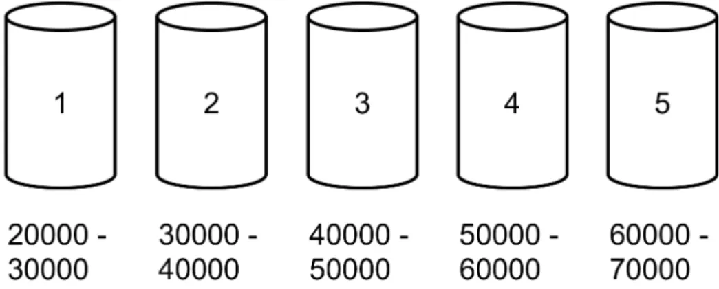
Bins is a simple way of mapping two variables. After an analysis that confirms that a mapping exists (e.g. correlation coefficient above or below threshold), we can create a number of bins. In a recommender system where explicit ratings are given by a value between one and five, we create five bins with different ranges according to the implicit ratings.

If we observe the following explicit-implicit rating pairs: (1 - 20 000), (3 - 45 000), (4 - 50 000) and (5 - 65 000), we clearly see that higher implicit value maps to higher explicit value. In this example, the explicit value is a rating between one and 5, and implicit rating is the time in milliseconds the user has spent reading an article. With equal size of each bin, the equation used to find the size of each bin is:

max−min

n (7.2)

where max and min is the highest and lowest implicit value accordingly and n

the number of different ratings. In our example, the size of each bin is (70000−

20000)/5 = 10000, and the range of each bin will look like the bins presented in Figure 7.2. A new rating without explicit, but with implicit rating of 55 000 will then be given four as explicit rating.

7.4 Linear Regression

Linear regression attempts to model the relationship between two variables by fit-ting a linear equation to observed data2_{. The two variables are called independent}

and dependent variables, where the independent variable in recommender systems

(54)

Figure 7.2: Example of bins with equal size

refers to implicit feedback and the dependent variable refers to explicit feedback. A linear regression line has an equation of the form

Y =a+bX (7.3)

whereX is the independent variable, Y the dependent variable, a is the intercept and b the slope of the line.

In the news domain, the dependent variableY is the rating while the independent variable can be the time a user spends reading the article. When Equation 7.3 has been fitted by observed data the equation can look like Equation 7.4. If we then want to map another article which only has a TimeOnPage as 55 000, we get a rating of 1.5 + 0.00005×55000 = 4.25≈4.

Rating = 1.5 + 0.00005·T imeOnP age (7.4)

When linear regression is used, an analysis that determines if there exists a rela-tionship between the two variables should be done. As discussed in Section 7.2, the correlation coefficient is a numerical measure of association between the variables, and can be used to determine if a relationship exists and ensure that it make sense to use linear regression.

7.4.1 Multiple Linear Regression

Multiple linear regression attempts to model the relationship between two or more independent variables and a dependent variable by fitting a linear equation to

(55)

Chapter 7 Mapping Techniques 41

observed data3_{. When we use multiple linear regression, the formula is}

Y =β0+β1X1+β1X1+...+βnXn (7.5)

where n is the number of independent variables and β describes how much each variable affects the regression line.

With multiple linear regression, we can expand Equation 7.4 with other implicit feedback such as the time a user moves the mouse when reading an article. With two such independent variables, the equation becomes:

Rating = 1.5 + 0.00005·T imeOnP age+ 0.0008·T imeOnM ouse (7.6)

Subsequently, an article that a user has spent 55 000 ms reading and 800 ms moving the mouse, will then get a rating of 1.5+0.00005×55000+0.0008×800 = 4.89≈5.

7.5 Classifiers

The mapping from implicit to explicit feedback can also be seen as a classification problem, where we want to find or classify an explicit rating based on a known set of mappings or instances. When we want to classify a rating from 1-5, we are able to use not only numeric predictors like regression models, but also classifiers normally working on nominal class values. A lot of research has been done on the task of classification, and a number of standard classification methods exist, where each has its own strengths and weaknesses. In this section we look at a set of classifiers with the feedback mapping in mind.

7.5.1 Naive Bayes Classification

Naive Bayes is a probabilistic classifier named after Bayes rule4_{, which assigns a}

class to an instance based on the highest estimated probability [24]. Given a fixed set of classes, for example rating 1-5, the classifier is trained by calculating the

3_{http://www.stat.yale.edu/Courses/1997-98/101/linmult.htm} 4_{http://en.wikipedia.org/wiki/Bayes’ theorem}

(56)

global probability for each class. The Naive Bayes classifier is so called because it assumes that the features in the data are independent of each other. It has, however, shown to perform well in many different environments[25]. When calcu-lating the likelihood of each class, apply the naive feature assumption to Bayes theorem given in equation 7.7. When assuming independence, we get Equation 7.8, often called the maximum a posteriori probability (MAP) where B denotes an implicit feedback variable such as time spent reading an article, and A denotes a rating. To classify, we then apply the argmax function, yielding the most probable classification. P(A|B) = P(B|A)P(A) P(B) (7.7) P(A|B)∝P(B) Y 1≤k≤nd P(tk|B) (7.8)

7.5.2 K-Nearest Neighbor

K-Nearest Neighbor (KNN)[26] is a very simple classification method, where we do not train a model, but simply assign the majority class of the K nearest neighboring instances. It is important to select an appropriate number of neighbors and which distance measure to use. When data sets become large, performance issues can occur. These can be mitigated to a degree by computing the similarity matrix prior to classification. There are many different distance measures that can be used, depending on the data set. Euclidean distance or cosine similarity are examples of common distance functions that can be applied to items with numeric data. Given vectorsxaand xb, the euclidean distance between these two vectors is given

in Equation 7.9. distance(xa, xb) = v u u t n X t=1 (xa,t−xb,t)2 (7.9)

7.5.3 Artificial Neural Network

An artificial neural network (ANN)[27] is a computational model devised from the human brain, and is often used to solve machine learning problems, including that

Collaborative Filtering in the News Domain with Explicit and Implicit Feedback