Aircraft navigation based on differentiation–integration observer

Aircraft navigation based on differentiation-integration observer

a _{Department of Electrical and Electronic Engineering, University of Nottingham,}

University Park, Nottingham, NG7 2RD, United Kingdom (Email: [email protected])

b _{Department of Mechanical and Aerospace Engineering,}

Hong Kong University of Science and Technology, Hong Kong, China (Email: [email protected])

Abstract: In this paper, a generalized differentiation-integration observer is presented based on sensors selection. The proposed differentiation-integration observer can estimate the multiple in-tegrals and high-order derivatives of a signal, synchronously. The parameters selection rules are presented for the differentiation-integration observer. The theoretical results are confirmed by the frequency-domain analysis. The effectiveness of the proposed observer are verified through the numerical simulations on a quadrotor aircraft: i) through the differentiation-integration observer, the attitude angle and the uncertainties in attitude dynamics are estimated synchronously from the measurements of angular velocity; ii) a control law is designed based on the observers to drive the aircraft to track a reference trajectory.

Keywords: Differentiation-integration observer, multiple integrals, derivatives, quadrotor aircraft

1

Introduction

Integration and differentiation are important components in almost all industrial applications. Their problems are of estimating the valuesI(a) =∫₀t· · ·∫₀sa(σ)dσ· · ·dτ andDi(a) = d

i_a(t)

dti . The positions, velocities and accelerations are the important elements for many systems. In an inertial navigation system (INS), the inertial measurement unit (IMU) typically measures the three-axial angular velocity and the three-axial linear acceleration, respectively. To obtain the attitude angle and angular acceleration of the device, the angular velocity signals are integrated and differentiated, respectively. For a long-time navigation, the drift phenomenon of INS is mainly brought out by the usual integration methods. They cannot restrain the effect of stochastic noise (especially non-zero mean noise). The noise leads to the accumulation of additional drift in the integrated signal.

The algorithms of differentiation and integration have been studied by a number of researchers [1]-[23]. The linear high-gain differentiators [2, 3] can provide the estimations of signal derivatives. In another study, a differentiator via high-order sliding modes algorithm was proposed [4, 5]. In [6]-[9], the continuous nonlinear differentiators based on finite-time stability were presented to provide the smooth estimations of signal derivatives. However, the differentiators did not consider the signal integral estimations [1]-[10].

18], the low-frequency differential differentiators [19, 20]. However, for the aforementioned integra-tors [12]-[20], only onefold integral was calculated, and the synchronous estimations of derivatives and integrals were not considered. Some integrators were implemented using the hardware units, where the circumstances usually affect the parameters, for instance, the temperature in the circuit changes. Thus, the estimation precisions are affected adversely. Moreover, they are easily infected by stochastic noise, and the drift phenomena are inevitable in such systems. In order to reduce the noise, additional filters must be added. In [21] and [22], a fractional-order integrator has been presented, and a rational transfer function was proposed to approximate the irrational integrator 1/sm. However, the limitation of 0< m <1 limits its application. The onefold and double integrals are necessary in many navigation systems. The Kalman filter can estimate position and velocity from the acceleration measurement [23]. However, it is supposed that the process noise covariance and measurement noise covariance are required to be zero-mean Gaussian distributed, and the pro-cess noise covariance is uncorrelated to the estimation error. These assumptions are different from the practical noise in signal. The inaccurate noise requirements may lead to the estimate drifts of position and velocity.

In [24], a nonlinear double-integral observer was presented to estimate synchronously the onefold and double integrals of a signal, and a generalized multiple integrator was designed to estimate the multiple integrals [25]. In [26], a nonlinear integral-derivative observer was proposed to estimate synchronously the integral and derivative of a signal. The parameters selection is required to be satisfied with Routh-Hurwitz Stability Criterion and the iterative equation relations. Moreover, the nonlinear observers in [26] are complicated and difficult to compute.The existing hardware computational circumstances affect the nonlinear function implementations adversely, i.e., the im-plementation of the these nonlinear observers in many digital processors is difficult. Due to the existence of such many parameters, the parameters regulation of this nonlinear observer is compli-cated.

In this paper, a generalized high-order linear differentiation-integration observer is presented, which can estimate the multiple integrals and high-order derivatives of a signal, synchronously. Different from the nonlinear observer theories in [26], the classical theory of linear system can be used to prove its stability, and the Bode plots are adopted to analyze its robustness. The parameters selection become relaxed, and it is only required to be satisfied with a simple Hurwitz condition. The existing layout of perturbation parameters in singular perturbation technique [27, 28] is only suitable to estimate the derivatives of a signal. In this differentiation-integration observer, a new distribution of perturbation parameters is presented for the requirement of synchronous estimation of the integrals and derivatives. The parameters selection rules and robustness analysis for the differentiation-integration observer are presented based on frequency-domain analysis.

provided. Moreover, quadrotor aircrafts are underactuated mechanical systems, and aerodynamic disturbance, unmodelled dynamics and parametric uncertainties are not avoidable in modeling. Based on the presented differentiation-integration observer, this paper provides a tracking control method for a quadrotor aircraft by using the measurements of position and angular velocity. The unknown velocity, attitude angle and uncertainties are reconstructed by the observers. Further-more, a controller is designed to stabilize the flight dynamics.

2

Generalized differentiation-integration observer

2.1 Configuration of differentiation-integration observer

The goal of the differentiation-integration observer design is to estimate the needed states from the different sensors, for instance:

1) Estimation of velocity and acceleration from position: In a GPS, position p(t) is known, we want to obtain the velocity and acceleration. Therefore, we expect to design an observer to estimate the first-order derivative ˙p(t) and second-order derivative ¨p(t) of the signal p(t), synchronously. The observer should include the state x = (x1, x2, x3), and the configuration of the observer is

described as follow:

˙

x1=x2; ˙x2 =x3;

˙

x3=f(x1−p(t), x2, x3) (1)

where the first state x1 of observer (1) points to the input signal p(t). If the state x1 estimates

p(t), and the system is stable, then, from the integral-chain relations ofx1, x2, x3 in system (1), the

first-order and second-order derivatives of signal p(t) can be estimated, synchronously.

2) Estimation of attitude angle and angular acceleration from angular velocity: In an IMU, an-gular velocity ω(t) can be measured directly. We want to obtain the attitude angle and angular acceleration. Therefore, we expect to design an observer to estimate the integral∫₀tω(σ)dσand the derivative ˙ω(t) of signalω(t), synchronously. The observer should include the statex= (x1, x2, x3),

and the configuration of the observer is shown as follow:

˙

x1=x2; ˙x2=x3;

˙

x3=f(x1, x2−ω(t), x3) (2)

where the second state x2 of observer (2) points to the input signal ω(t). If the statex2 estimates

ω(t), and the system is stable, then, from the integral-chain relations of x1, x2, x3 in system (2),

the onefold integral and first-order derivative of signalω(t) can be estimated, synchronously.

3) Estimation of position and velocity from acceleration: In the third case, the accelerationac(t)

is measured by a accelerometer, and we want to obtain the position and the velocity. There-fore, we expect to design an observer to estimate the onefold integral ∫₀tac(σ)dσ and the double

integral ∫₀t∫₀sac(σ)dσdτ of signal ac(t), synchronously. The observer should include the state

˙

x1=x2; ˙x2=x3;

˙

x3=f(x1, x2, x3−ac(t)) (3)

where the third state x3 of observer (3) points to signalac(t). If the state x3 estimates ac(t), and

the system is stable, then, from the integral-chain relations ofx1, x2, x3 in system (3), the onefold

and double integrals of signal ac(t) can be estimated, synchronously.

4) Generalized cases: Generally, for signal a(t) measured from a sensor, we expect to design an observer to estimate the multiple integrals up to (p−1)th multiple and high-order derivatives up to (n−p)th order, synchronously, where p∈ {1,· · · , n} corresponds to different sensors. Let the ith-multiple integral of signal a(t) be Ip−i(t) =

∫ t

0

· · ·

∫ s

0

| {z }

i

a(σ)dσ_{| {z }}· · ·dτ

i

, where i∈ {1,· · · , p−1};

Ip(t) =a(t); and the (r−p)th-order derivative of signala(t) beIr(t) =a(r−p)(t),r=p+ 1,· · ·, n.

The observer should include the statex= (x1,· · ·, xp,· · · , xn), and the configuration of the observer

is presented as follow:

˙ x1=x2

· · ·

˙

xp=xp+1

· · ·

˙

xn=f(x1,· · ·, xp−a(t),· · ·, xn) (4)

where the p-th state xp of observer (4) points to signal a(t). If the state xp estimates a(t), and

the system is stable, then, from the integral-chain relations ofx1,· · · , xp,· · ·, xnin system (4), the

multiple integrals and high-order derivatives of signal a(t) can be estimated, synchronously. The goals of the observation are: 1) synchronous estimation of multiple integrals and high-order derivatives of a signal; 2) regulation of low-pass frequency bandwidth through the ease of parameter selection, and sufficient high-frequency noise rejection.

2.2 Existence conditions of Hurwitz characteristic polynomial

Before constructing the explicit form of the differentiation-integration observer (4), we propose a nth-order characteristic polynomial

sn+knsn−1+· · ·+

kp

εp−c(p)s

p−1_{+· · ·+k}

2s+k1 (5)

where, p∈ {1,· · · , n}, and

c(p) = {

1, p= 1

0, p >1 (6)

arbitraryε∈(0,1), by selecting parametersk1,· · ·,kn, whether can all the positive integersnand

p∈ {1,· · · , n}make the polynomial (5) Hurwitz?

For instance, we can find that: 1) for the arbitraryε∈(0,1), when we selectn= 4 and p= 2, the polynomial (5) cannot be Hurwitz; 2) for the arbitrary ε∈(0,1), when n= 5 and p∈ {2,3,4,5}, the polynomial (5) cannot be Hurwitz.

For the arbitrary ε ∈ (0,1), the following lemma presents the selections of n and p to make polynomial (5) Hurwitz.

Lemma 1: For the arbitraryε∈(0,1), in the following cases, the polynomial (5) can be Hurwitz: a) n∈ {1,2,· · · } and p = 1: ki >0 (where i= 1,· · ·, n) are selected such that the polynomial

sn+

n

∑

i=1

kisi−1 is Hurwitz.

b) n= 2 and p= 2: k1>0, k2>0.

c) n= 3 and p ∈ {2,3}: when p= 2, k1 >0, k3 >0 and k2 > ε2k_k1₃; when p = 3,k1 >0, k3 >0

and k2> ε3k_k1₃.

d) n= 4 and p= 3: k1>0, k4>0, k3> ε3k_k2₄ and k2 > ε3 k2

4k1+k22

k4k3 .

The proof of Lemma 1 is presented in Appendix.

2.3 Design of generalized differentiation-integration observer

In the following, the singular perturbation technique will be used to design a generalized differentiation-integration observer, and Theorem 1 is presented as follow.

Theorem 1: For system

˙

xi=xi+1;i= 1,· · ·, n−1

εn+1−c(p)x˙n=− n

∑

i=1,i̸=p

kiεi−c(p)xi−kp(xp−a(t)) (7)

where, p∈ {1,· · · , n}, and

c(p) = {

1, p= 1

0, p >1 (8)

a(t) is the signal that can be directly measured, and it is continuous, integrable and (n−p+ 1)th-order derivable. Let ap−i(t) =

∫ t

0

· · ·

∫ s

0

| {z }

i

a(σ)dσ_{| {z }}· · ·dτ

i

,i ∈ {1,· · · , p−1}; ap(t) = a(t); ar(t) =

a(r−p)(t),r =p+ 1,· · · , n;ε∈(0,1) is the perturbation parameter; k1,· · ·,_εp−kcp(p),· · ·, kn>0 are

selected such that sn+knsn−1+· · ·+ _εp−kcp(p)sp−1+· · ·+k2s+k1 is Hurwitz, then the following

conclusions hold:

lim

ε→0xi =ai(t),fori∈ {1,· · · , n} (9)

Proof: The Laplace transformation of (7) can be calculated as follow:

sXi(s) =Xi+1(s) ;i= 1,· · · , n−1

εn+1−c(p)sXn(s) =− n

∑

i=1,i̸=p

kiεi−c(p)Xi(s)−kp(Xp(s)−A(s)) (10)

where Xi(s) and A(s) denote the Laplace transformations of xi and a(t), respectively, and s

denotes Laplace operator. From (10), we obtain

Xi(s) =

Xj(s)

sj−i , i= 1,· · · , n, j∈ {1,· · ·, n} (11)

Therefore, Eq. (10) can be written as

sn−j+1εn+1−c(p)Xj(s) =− n

∑

i=1,i̸=p

kiεi−c(p)

Xj(s)

sj−i −kp

( Xj(s)

sj−p −A(s)

)

(12)

Then, it follows that

Xj(s)

A(s) =

kp

sn−j+1_εn+1−c(p)₊ ∑n i=1,i̸=p

kiεi−c(p)

sj−i +

kp

sj−p

(13)

i.e.,

Xj(s)

A(s) =

sj−1kp

sn_εn+1−c(p)₊ ∑n i=1,i̸=p

si−1_k

iεi−c(p)+sp−1kp

(14)

Therefore, we obtain

lim

ε→0

Xj(s)

A(s) =s

j−p ₍₁₅₎

where j ∈ {1,· · · , n} and p ∈ {1,· · ·, n}. It means that the state xi approximates ai(t), for

1≤i≤n.

From Eq. (14), the characteristic polynomial of observer (7) is

sn+

n

∑

i=1,i̸=p

ki

εn−i+1s

i−1₊kp/εp−c(p)

εn−p+1 s

p−1 ₍₁₆₎

Importantly, in order to make the system stable, the characteristic polynomial is required to be Hurwitz. It is equivalent that

sn+

n

∑

i=1,i̸=p

kisi−1+

kp

εp−c(p)s

p−1 ₍₁₇₎

From Theorem 1, we find that: the statexp estimates the signala(t), xi estimates the (p−i

)th-multiple integral of signal a(t), where i ∈ {1,· · · , p−1}; xr estimates the the (r −p)th-order

derivative of signala(t), where r=p+ 1,· · · , n.

2.4 Explicit forms of differentiation-integration observers

From Theorem 1 and Lemma 1, the explicit forms of generalized differentiation-integration ob-server can be deduced, and a corollary is presented as follow. It includes: high-order differentia-tor, onefold integradifferentia-tor, differentiation-integration observer, double integradifferentia-tor, differentiation and double-integration observer.

Corollary 1: The following differentiation-integration observers exist:

i) High-order differentiator [35] (where n∈ {1,2,· · · }and p= 1):

˙

xi=xi+1;i= 1,· · · , n−1

εnx˙n=−k1(x1−a(t))− n

∑

i=2

kiεi−1xi (18)

where, ε ∈ (0,1); ki > 0 (i = 1,· · ·, n) are selected such that the polynomial sn+ n

∑

i=1

kisi−1 is

Hurwitz. For differentiator (18), the following conclusions hold:

lim

ε→0xi =a

(i−1)_{(t),fori∈ {1,· · · , n} (19)}

It can estimate the derivatives of signala(t) up to (n−1)th order.

ii) Onefold integrator(where n= 2 and p= 2):

˙ x1=x2

ε3x˙2=−k1εx1−k2(x2−a(t)) (20)

where, ε∈(0,1);k1>0, k2>0. The following conclusions hold:

lim

ε→0x1=

∫ t

0

a(t)dτ,lim

ε→0x2=a(t) (21)

It can estimate the onefold integral of signal a(t).

iii) Differentiation-integration observer (where n= 3 and p= 2):

˙ x1=x2

˙ x2=x3

where, ε∈(0,1);k1>0, k3>0 and k2 > ε2k_k1₃. The following conclusions hold:

lim

ε→0x1 =

∫ t

0

a(t)dτ,lim

ε→0x2 =a(t),εlim→0x3 = ˙a(t) (23)

It can estimate the onefold integral and the first-order derivative of signal a(t), respectively.

iv) Double integrator (where n= 3 and p= 3):

˙ x1=x2

˙ x2=x3

ε4x˙3=−k1εx1−k2ε2x2−k3(x3−a(t)) (24)

where, ε∈(0,1);k1>0, k3>0 and k2 > ε3k_k1₃. The following conclusions hold:

lim

ε→0x1=

∫ t

0

∫ τ

0

a(s)dsdτ,lim

ε→0x2 =

∫ t

0

a(τ),lim

ε→0x3=a(t) (25)

It can estimate the onefold and double integrals of signal a(t), respectively.

v) Differentiation and double-integration observer (where n= 4 and p= 3)

˙ x1=x2

˙ x2=x3

˙ x3=x4

ε5x˙4=−k1εx1−k2ε2x3−k3(x3−a(t))−k4ε4x4 (26)

where, ε∈(0,1);k1>0, k4>0, k3 > ε3k_k2₄ and k2 > ε3 k2

4k1+k22

k4k3 . The following conclusions hold:

lim

ε→0x1=

∫ t

0

∫ τ

0

a(s)dsdτ,lim

ε→0x2=

∫ t

0

a(τ),lim

ε→0x3 =a(t),εlim→0x4= ˙a(t), (27)

It can estimate the onefold, double integrals and the first-order derivative of signala(t), respectively.

3

Frequency analysis and parameters selection

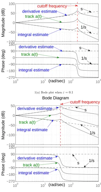
−100 −50 0 50 100

Magnitude (dB)

100 101 102 103

−270 −180 −90 0 90 180

Phase (deg)

Bode Diagram

(rad/sec)

derivative estimate

track a(t)

integral estimate

s

1/s

derivative estimate

track a(t)

integral estimate

s

1/s

cutoff frequency

1(a) Bode plot whenε= 0.1

−150 −100 −50 0 50

Magnitude (dB)

100 101 102 103

−270 −180 −90 0 90 180

Phase (deg)

Bode Diagram

(rad/sec)

derivative estimate

_s

track a(t)

integral estimate

1/s

derivative estimate

track a(t)

integral estimate

s

1/s

cutoff frequency

1(b) Bode plot whenε= 0.2

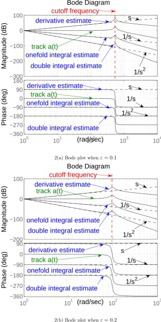
−300 −200 −100 0 100

Magnitude (dB)

100 101 102 103 104

−360 −270 −180 −90 0 90 180

Phase (deg)

Bode Diagram

(rad/sec)

derivative estimate

track a(t)

onefold integral estimate

double integral estimate

s

1/s

1/s

derivative estimate

track a(t)

onefold integral estimate

double integral estimate

s

1/s

1/s

cutoff frequency

2(a) Bode plot whenε= 0.1

−200 −100 0 100

Magnitude (dB)

100 101 102 103

−360 −270 −180 −90 0 90

Phase (deg)

Bode Diagram

(rad/sec)

derivative estimate

track a(t)

onefold integral estimate

double integral estimate

1/s

1/s

derivative estimate

track a(t)

onefold integral estimate

double integral estimate

s

s

1/s

1/s

cutoff frequency

2(b) Bode plot whenε= 0.2

3.1 Frequency characteristic with different perturbation parameter ε

1) Differentiation-integration observer (22)

For transfer function (14), let n= 3, p= 2, we obtain

Xj(s)

A(s) =

k2sj−1

ε4_s3_+ε3_k

3s2+k2s+εk1

, j∈ {1,2,3} (28)

where, k1 = 0.1, k2 = 3, k3 = 2, Selecting ε = 0.1 and ε = 0.2, the Bode plots for the transfer

function are described as Figs. 1(a) and 1(b), respectively.

2) Differentiation and double-integration observer observer (26)

For transfer function (14), let n= 4, p= 3, we obtain

Xj(s)

A(s) =

k3sj−1

ε5_s4_+ε4_k

4s2+k3s2+ε2k2s+εk1

, j ∈ {1,2,3,4} (29) where, k1 = 0.01, k2 = 0.1, k3 = 3, k4 = 2, Selectingε= 0.1 and ε= 0.2, the Bode plots for the

transfer function are described as Figs. 2(a) and 2(b), respectively.

Comparing with the ideal derivative operator s, the ideal integral operator 1/s and 1/s2_{, not}

only the presented differentiation-integration observers can obtain their estimations accurately, but also the high-frequency noise is rejected sufficiently (While in Figs. 1 and 2, the dash-lines represent the ideal operators and the solid lines represent the proposed observers). From Figs. 1 and 2, after the cutoff frequency lines, the estimations attenuate rapidly, and the high-frequency noises are also reduced sufficiently. Parameterεaffects the low-pass frequency bandwidth (See the cutoff frequency lines in Figures 1 and 2): Decreasing the perturbation parameter ε, the low-pass frequency bandwidth becomes larger, and the estimation speed becomes fast; on the other hand, increasing perturbation parameterε, the low-pass frequency bandwidth becomes smaller, and much noise can be rejected sufficiently (See the cases ofε= 0.1 andε= 0.2 in Figs.1 and 2, respectively).

3.2 The proposed rules of parameters selection

For the differentiation-integration observers, there are some rules suggested on the parameters selection:

1) The parameters ki (i = 1,· · · , n) decide the observer stability, and they should be satisfied

with the conditions in Lemma 1. Importantly, the selection of ki (i= 1,· · · , n) should make the

real parts of all the eigenvalues of polynomial (5) negative for the smallε∈(0,1).

a. For onefold integrator (20), the characteristic polynomial is s2 + k2/ε2

ε s+

k1

ε2 (See Eq. (16)

when n = 2 and p = 2). In fact, for ε ∈ (0,1), the eigenvalues of the equivalent characteristic polynomial s2 + k2

ε2s+k1 (See Eq. (17) when n = 2 and p = 2) can be written as the following

form: −a1, −a2 (The real eigenvalues of the characteristic polynomial for observer (20) are −a_ε1,

−a2

ε ). Therefore, this polynomial can be written as

s2+k2

ε2s+k1= (s+a1)(s+a2) =s 2_{+ (a}

1+a2)s+a1a2 (30)

By solving the above equation, it follows that

From Eq. (14), the transfer function of the onefold integrator (20) can be describled as

X2(s)

A(s) =

sk2

ε3_s2_+sk

2+k1ε

= sk2/ε

3

s2_+sk

2/ε3+k1/ε2

(31)

Then its nature frequency is

ωn=

√

k1/ε2 (32)

Based on the requirement of filtering high-frequency noise, the perturbation parameter can be selected as

ε=√k1/ω2n (33)

Because the drift is slow, the corresponding eigenvalue is selected to approach the imaginary axis with respect to the other eigenvalue. For example, let the eigenvalues be−a1 =−100,−a2=−0.02,

and select ωn= 8. Then we obtain the observer parameters as follows:

k1= 100×0.02 = 2

ε= 0.1768

k2= (100 + 0.02)×(2/64) = 3.1256

b. For the double integrator (24) (when n = 3 and p = 3), the characteristic polynomial is s3+k3/ε3

ε s

2₊k2

ε2s+k_ε31 (See Eq. (16) whenn= 3 andp= 3). In fact, forε∈(0,1), the eigenvalues

of this equivalent characteristic polynomials3+k3

ε3s2+k2s+k1(See Eq. (17) whenn= 3 andp= 3)

can be written as the following form: −a1, −a21+a22i, −a21−a22i (The real eigenvalues of the

characteristic polynomial for observer (24) are−a1

ε,−

a21

ε +

a22

ε i,−

a21

ε −

a22

ε i), wherea1, a21, a22>0.

Two conjugate eigenvalues are supposed to exist in this polynomial. Therefore, the polynomial s3+k3

ε3s2+k2s+k1 can be written as

s3+ k3 ε3s

2_+k

2s+k1= (s+a1)(s+a21+a22i)(s+a21−a22i) (34)

By solving the above equation, it follows that

k1 =a1(a221+a222), k2 =a221+a222+ 2a1a21, k3 =ε3(a1+ 2a21) (35)

It means that, after selecting the suitable eigenvalues −a1,−a21+a22i,−a21−a22iand εbased

on Bode plot analysis, the parametersk1,k2 andk3 can be calculated. Because the drifts are slow,

the corresponding eigenvalues are selected to approach the imaginary axis with respect to the other eigenvalues.

For example, selecting the eigenvalues of the polynomial as−46.8218,−0.0266+0.0999i,−0.0266− 0.0999i, and ε = 0.4, then k1 = 0.5, k2 = 2.5, k3 = 3; selecting the eigenvalues as −15.6190,

−0.0030 + 0.0800i,−0.0030−0.0800i, andε= 0.4, thenk1 = 0.1,k2 = 0.1,k3 = 1. Obviously, the

c. For differentiation-integration observer (22) (when n = 3 and p = 2), the characteristic polynomial iss3+k3

ε s2+

k2/ε2

ε2 s+k_ε13 (See Eq. (16) when n= 3 and p= 2). In fact, forε∈(0,1),

the eigenvalues of the equivalent characteristic polynomial s3+k3s2+_εk22s+k1 (See Eq. (17) when

n = 3 and p = 2) can be written as the following form: −a11 +a12i, −a11−a12i, −a2, (The

real eigenvalues of the characteristic polynomial for observer (22) are −a11

ε +

a12

ε i, −

a11

ε −

a12

ε i,

−a2

ε ), wherea11, a12, a1 >0. Two conjugate eigenvalues are supposed to exist in this polynomial.

Therefore, the polynomial s3_+k

3s2+ k_ε22s+k1 can be written as

s3+k3s2+

k2

ε2s+k1= (s+a11+a12i)(s+a11−a12i)(s+a2) (36)

By solving the above equation, it follows that

k1 = (a211+a212)a2, k2 =ε2(a211+a212+ 2a11a2), k3= 2a11+a2 (37)

It means that, after selecting the suitable eigenvalues −a11+a12i,−a11−a12i,−a2 and εbased

on Bode plot analysis, the parameters k1,k2 and k3 can be calculated.

2) In order to increase the estimation speed,ε∈(0,1) should decrease to make the low-pass fre-quency bandwidth larger; if much noise exists,εshould increase, the low-pass frequency bandwidth becomes smaller, and the noise can be rejected sufficiently.

3) It is easy to see that the k-fold integrator provides for a much better accuracy of ith-fold integral than the l-fold integrator, where, k > l and i = 1,· · · , l−1. For instance, the double integrator (24) provides for a much better accuracy of onefold integral than the onefold integrator (20).

4) It is easy to see that the kth-order differentiator provides for a much better accuracy of i th-order derivative than thelth-order differentiator, where,k > landi= 1,· · · , l−1. For instance, in the high-order differentiator (18), the third-order differentiator (where n= 3) provides for a much better accuracy of first-order derivative than the second-order differentiator (where n= 2).

4

Estimations by onefold integrator and double integrator

In this section, we use the simulations to illustrate the effectiveness of the proposed observers. The estimation performances of the presented observers are compared with Extended Kalman Filter (EKF) [23], and a long-time simulation is described to investigated their drift phenomena.

1) Estimation by onefold integrator (20)

In this section, the onefold integrator (20), i.e.,

˙ x1=x2

ε3x˙2=−k1εx1−k2(x2−a(t))

0 20 40 60 80 100 −2

−1 0 1 2

time(s)

input signal

0 20 40 60 80 100

−0.5 0 0.5 1

time(s)

noise

a(t)

a

02(t)

noise

3(a) Input signal

0 20 40 60 80 100

−2 −1 0 1 2

time(s)

signal estimate

0 20 40 60 80 100

−0.5 0 0.5 1

time(s)

estimate error

x₂

a₀₂(t)

error of x

2 and a02(t)

3(b) Signal estimate

0 20 40 60 80 100

−1 0 1 2

time(s)

onefold integral

0 20 40 60 80 100

−0.2 0 0.2 0.4 0.6

time(s)

estimate error

x₁

a

01(t) integral by EKF

error of x

1 and a01(t) _{error by EKF}

3(c) Onefold integral estimate

Figure 3 Estimation by onefold integrator (20) in 100s

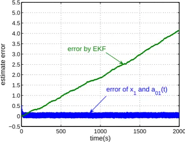
0 500 1000 1500 2000

−0.5 0 0.5 1.0 1.5 2.0 2.5 3.0 3.5 4.0 4.5 5.0 5.5

time(s)

estimate error

error of x

1 and a01(t) error by EKF

0 20 40 60 80 100 −2

−1 0 1 2

time(s)

input signal

0 20 40 60 80 100

−0.5 0 0.5 1

time(s)

nonise

a(t)

a

03(t)

noise

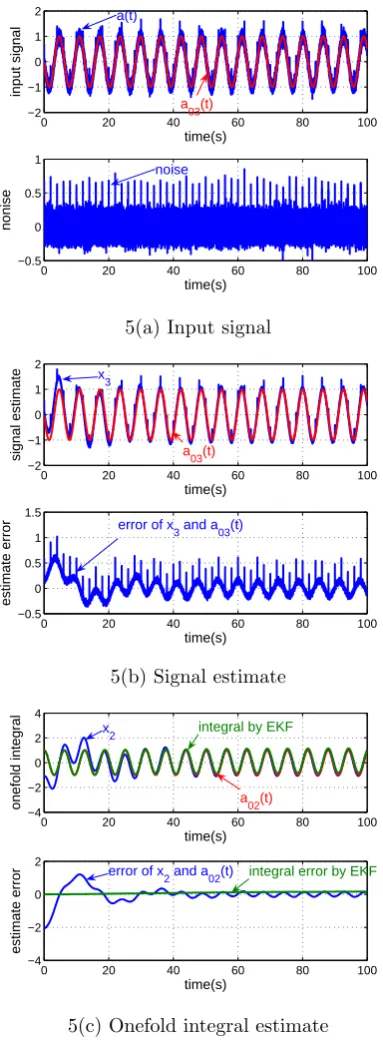
5(a) Input signal

0 20 40 60 80 100

−2 −1 0 1 2

time(s)

signal estimate

0 20 40 60 80 100

−0.5 0 0.5 1 1.5

time(s)

estimate error

x₃

a

03(t)

error of x

3 and a03(t)

5(b) Signal estimate

0 20 40 60 80 100

−4 −2 0 2 4

time(s)

onefold integral

0 20 40 60 80 100

−4 −2 0 2

time(s)

estimate error

x

2

a

02(t) integral by EKF

error of x

2 and a02(t) integral error by EKF

5(c) Onefold integral estimate

0 20 40 60 80 100

−10 −5 0 5 10

time(s)

double integral

0 20 40 60 80 100

−10 −5 0 5 10

time(s)

estimate error

x

1 double integral by EKF

a₀₁(t)

double integral error by EKF

error of x

1 and a01(t)

5(d) Double integral estimate

0 500 1000 1500 2000 −3

−2 −1 0 1 2 3 4 5

time(s)

estimate error

error of x

2 and a02(t) integral error by EKF

6(a) Onefold integral estimate

0 500 1000 1500 2000

−500 0 500 1000 1500 2000 2500 3000 3500 4000 4500 5000

time(s)

estimate error

error of x

1 and a01(t) double integral error by EKF

6(a) Double integral estimate

6 Comparison of double integrator (24) and EKF in 2000s

Here, the stochastic non-zero mean noise is selected, and the mean value of the noise is not equal to zero (See the noise in Fig. 3(a)). The non-zero mean noiseδ(t) consists of following two signals: Random number with Mean=0, Variance=0.01, Initial speed=0, and Sample time=0; Pulses with Amplitude=0.5, Period=2s, Pulse width=1, and Phase delay=0.

The signal a02(t) = cos(t) is selected as the reference signal, and a(t) = a02(t) +δ(t) +d(t).

Therefore, a01 =

∫t

0a(τ)dτ = sin(t). Integrator parameters: k1 = 2, k2 = 2.7783, ε = 0.1667.

Suppose the initial state is (x1(0), x2(0)) = (0.5,2). In the onefold integrator (20), x2 estimates

signal a02(t), x1 estimate the onefold integral a01(t). Signal a02(t) tracking, the onefold integral

estimation in 100 seconds are presented in Fig. 3. Fig. 3(a) provides signala02(t) with stochastic

noise. Fig. 3(b) describes signal a02(t) estimation. Fig. 3(c) presents the comparison of onefold

integral estimation by onefold integrator (20) and Extended Kalman filter [23]. Figs. 4 describes the estimation comparison in 2000 seconds.

2) Estimation by double integrator (24)

In this section, the double integrator (24), i.e.,

˙ x1=x2

˙ x2=x3

ε4x˙3=−k1εx1−k2ε2x2−k3(x3−a(t))

is used to estimate the onefold and double integrals from the signal a(t) in spite of the existence of stochastic non-zero mean noise δ(t) and measurement error d(t).

Here, the stochastic non-zero mean noise in 1) is selected.

The signal a03(t) = −sin(t) is selected as the reference signal, and a(t) = a03(t) +δ(t) +d(t).

Therefore, a02=

∫t

0a03(σ)dσ= cos(t), anda01=

∫t 0

∫s

0 a(σ)dσdτ = sin(t).

The double integrator parameters: k1 = 0.5, k2 = 2.5,k3 = 3, ε= 0.4. Suppose the initial state

is (x1(0), x2(0), x3(0)) = (0.1,−1.1,0.1). In the double integrator (24), x3 tracks signal a03(t), x2

and x1 estimate the onefold and double integrals of signala03(t), respectively.

Signal a03(t) tracking, the onefold and double integral estimations in 100 seconds are presented

in Fig. 5. Fig. 5(a) provides signal a03(t) with stochastic noise. Fig. 5(b) describes a03(t)

estimation. Figs. 5(c) and 5(d) present the comparisons of onefold and double integral estimations by the double integrator (24) and the Extended Kalman filter [23]. Figs. 6(a)-6(b) describe the estimation comparisions of in 2000 seconds.

From Figs. 5(c), 5(d), 6(a) and 6(b), the obvious estimation drifts of onefold and double integrals exist by the Extended Kalman filter. With respect to the Extended Kalman filter, despite the existence of the intensive non-zero mean stochastic noise, the proposed double integrator (24) showed the promising estimation ability and robustness. Furthermore, from Figs. 6(a)-6(b), no drift phenomenon happened in the long-time estimations.

5

Application to quadrotor aircraft

In this paper, the mathematical model and reference trajectory of the quadrotor aircraft described in [29] are used. The description of forces and torques of the quadrotor aircraft is shown in Fig. 7 [29].

F2

F1

F3

F4

C

mg Exb Eyb

Ezb

Ez

Ex Ey

Q1

Q3

Q2

Q4

Let Ξg = (Ex, Ey, Ez) denote the right handed inertial frame, and Ξb =

(

E_xb, E_yb, E_zb) denote the frame attached to the aircraft’s fuselage whose origin is at the center of gravity. (ψ, θ, ϕ) denotes the aircraft orientation expressed in the yaw, pitch and roll angles (Euler angles). The symbol cθ

is used for cosθand sθ for sinθ. Rbg is the transformation matrix from the frame Ξb to Ξg, and

Rbg =

  

cψcθ sψcϕ+cψsθsϕ sψsϕ−cψsθcϕ

−sψcθ cψcϕ−sψsθsϕ cψsϕ+sψsθcϕ

sθ −cθsϕ cθcϕ

 

 (38)

For the quadrotor aircraft, the right–left rotors rotate clockwise and the front-rear ones rotate counterclockwise (See Fig. 7). The rotational directions of the rotors do not change (i.e., ωi >0,

i ∈ {1,2,3,4}). The reactive torque generated by the rotor i due to the rotor drag is Qi =kω2i,

and the total thrust generated by the four rotors is F =

4

∑

i=1

Fi = b 4

∑

i=1

ω2_i, where Fi = bωi2 is the

lift generated by the rotor iin free air, andk, b >0 are two parameters depending on the density of air, the size, shape, and pitch angle of the blades, as well as other factors. Therefore, we obtain Qi = k_bFi, i= 1,2,3,4. Thus the sum reactive torque generated by the four rotors due to the rotor

drags isQ=

4

∑

i=1

(−1)iQi = k_b 4

∑

i=1

(−1)iFi.

The motion equations in the coordinate (x, y, z) are then [29]

mx¨= (sψsϕ−cψsθcϕ)F−kxx˙+δx

my¨= (cψsϕ+sψsθcϕ)F−kyy˙+δy

mz¨=cθcϕF−mg−kzz˙+δz (39)

Jzψ¨=

k b

4

∑

i=1

(−1)iFi−kψψ˙+δψ

Jyθ¨= (F1−F3)l−lkθθ˙+δθ

Jxϕ¨= (F2−F4)l−lkϕϕ˙+δϕ (40)

where, m is the mass of the aircraft; g is the gravity acceleration;Jx,Jy and Jz are the three-axis

moment of inertias; kx, ky, kz, kψ, kθ and kϕ are the drag coefficients; l is the distance between

each rotor and the center of gravity. δx,δy and δz are the bounded disturbances and uncertainties

in position dynamics; δψ, δθ and δϕ are the bounded disturbances and uncertainties in attitude

dynamics.

Here, for the quadrotor aircraft, we are interested in designing the observers to estimate ( ˙x, ˙y, ˙z, ψ,θ,ϕ) and the uncertainties (kx,ky,kz,kψ,kθ,kϕ) and (δx,δy,δz,δψ,δθ,δϕ) from the information

of (x, y, z, ˙ψ, ˙θ, ˙ϕ). Moreover, based on these observers, the controllers Fi (i= 1,2,3,4) will be

designed to implement: x→ xd, ˙x→ x˙d, y →yd, ˙y→ y˙d, z→ zd, ˙z→ z˙d, andψ →ψd, ˙ψ→ψ˙d,

θ→θd, ˙θ→θ˙d,ϕ→ϕd,ϕ→ϕ˙dast→ ∞.

5.1 Observer designs for the quadrotor aircraft

directly, (kx, ky,kz,kψ, kθ, kϕ) and (δx,δy,δz,δψ,δθ,δϕ) are bounded and unknown. Select the

auxiliary controller vector as

up =

  

upx

upy

upz

  =

  

sψsϕ−cψsθcϕ

cψsϕ+sψsθcϕ

cθcϕ

 

F (41)

Then we can find that

F =∥up∥₂ =

√ u2

px+u2py+u2pz (42)

That is to say, after designing (upx, upy, upz), F can be calculated. Therefore, (upx, upy, upz) is

known. Let [29]

h1(t) =

upx

m , h2(t) = upy

m , h3(t) = upz

m −g, h4(t) =

k Jzb

4

∑

i=1

(−1)iFi, h5(t) =

l Jy

(F1−F3), h6(t) =

l Jx

(F2−F4) (43)

d1(t) = (δx−kxx˙)/m, d2(t) = (δy−kyy˙)/m,

d3(t) = (δz−kzz˙)/m, d4(t) = (δψ−kψψ˙)/Jz,

d5(t) = (δθ−lkθθ˙)/Jy, d6(t) = (δϕ−lkϕϕ˙)/Jx (44)

w1,1=x, w2,1=y, w3,1 =z, w4,1 =ψ, w5,1 =θ, w6,1 =ϕ

w1,2= ˙x, w2,2= ˙y, w3,2 = ˙z, w4,2 = ˙ψ, w5,2 = ˙θ, w6,2 = ˙ϕ (45)

then the position dynamics (39) can be rewritten as

˙

wi,1=wi,2

˙

wi,2=hi(t) +di(t)

yopi=wi,1 (46)

where i= 1,2,3, and the attitude dynamics (40) can be given by

˙

wi,1=wi,2

˙

wi,2=hi(t) +di(t)

yopi=wi,2 (47)

where i= 4,5,6.

1) The third-order differentiator (18) for velocity and uncertainties estimate in position dynamics

The following corollary gives the observers to estimate ( ˙x,y,˙ z˙) and uncertainties in the position dynamics.

Corollary 2: The observer (18) (where n= 3) are designed for aircraft position dynamics (39) as follows:

˙

xi,1=xi,2

˙

xi,2=xi,3

ε3_ix˙i,3=−k1(xi,1−wi,1)−k2εixi,2−k3ε2ixi,3 (48)

wherei= 1,2,3. From (x, y, z), we can estimate ( ˙x,y,˙ z˙) anddi(t) (i= 1,2,3) by the differentiators

in Eq. (48), and the following conclusions hold:

lim

ε→0x1,1=x,εlim→0x1,2 = ˙x,εlim→0x1,3−h1(t) =d1(t)

lim

ε→0x2,1=y,εlim→0x2,2= ˙y,εlim→0x2,3−h2(t) =d2(t)

lim

ε→0x3,1=z,εlim→0x3,2 = ˙z,εlim→0x3,3−h3(t) =d3(t) (49)

2) Differentiation-integration observer (22) for attitude angle estimation

The following corollary gives the observers to estimate (ψ, θ, ϕ) and uncertainties in the attitude dynamics.

Corollary 3: The differentiation-integrator observers are designed for aircraft attitude dynamics (40) as follows:

˙

xi,1=xi,2

˙

xi,2=xi,3

ε4_ix˙i,3=−ki,1εixi,1−ki,2(xi,2−wi,2)−ki,3ε3ixi,3 (50)

wherei= 4,5,6. From ( ˙ψ,θ,˙ ϕ˙), we can estimate (ψ, θ, ϕ) anddi(t) (i= 4,5,6) by the

differentiation-integration observers in Eq. (50), and the following conclusions hold:

lim

ε→0x4,1=ψ,εlim→0x4,2 = ˙ψ,εlim→0x4,3−h4(t) =d4(t)

lim

ε→0x5,1=θ,εlim→0x5,2 = ˙θ,εlim→0x5,3−h5(t) =d5(t)

lim

ε→0x6,1=ϕ,εlim→0x6,2 = ˙ϕ,εlim→0x6,3−h6(t) =d6(t) (51)

5.2 Controller design

For reference trajectory (xd, yd, zd), define e1 = x−xd, e2 = ˙x−x˙d, e3 = y−yd, e4 = ˙y−y˙d,

e5 =z−zd, and e6 = ˙z−z˙d. The system error for position dynamics (39) can be written as

¨

ep =m−1(up+ Ξp+δp) (52)

where

ep=

[ e1e3e5

]T

,Ξp=

  

−mx¨d

−my¨d

−mz¨d−mg

  , δp =

  

δx−kxx˙

δy−kyy˙

δz−kzz˙

 

 (53)

For reference attitude angle (ψd, θd, ϕd), definee7 =ψ−ψd,e8= ˙ψ−ψ˙d,e9=θ−θd,e10= ˙θ−θ˙d,

e11=ϕ−ϕd,e12= ˙ϕ−ϕ˙d. The system error for attitude dynamics (40) is given by

¨

ea=J−1(ua+ Ξa+δa) (54)

where

ea=

   e7 e9 e11   , ua=

     k b 4 ∑ i=1

(−1)iFi

(F1−F3)l

(F2−F4)l

    ,Ξa=

  

−Jzψ¨d

−Jyθ¨d

−Jxϕ¨d

  , δa=

  

δψ−kψψ˙

δθ−lkθθ˙

δϕ−lkϕϕ˙

 

, J =diag{Jz, Jy, Jx}

(55)

5.2.1 Controller design for position dynamics

Theorem 2: For the position dynamics (39), to track the reference trajectory (xd, yd, zd), if the

controller is selected as

up =−Ξp−bδp−m(kp1bep+kp2be˙p) (56)

wherebe1 =bx−xd,eb2 =bx˙−x˙d,be3 =yb−yd,be4 =yb˙−y˙d,be5 =zb−zd,be6=bz˙−z˙d;kp1, kp2>0, and

b ep =

   b e1 b e3 b e5   ,be˙p =

   b e2 b e4 b e6   ,δbp=

  

x1,3

x2,3

x3,3

 

 (57)

then the position error dynamics (52) rendering by controller (56) will converge asymptotically to the origin, i.e., the tracking errors ep →0 and ˙ep →0 ast→ ∞.

The proof of Theorem 2 is presented in Appendix.

From (41), (42) and (56), we obtain

F =−Ξp−bδp−m(kp1bep+kp2be˙p)

5.2.2 Controller design for attitude dynamics

Theorem 3: For the attitude dynamics (40), to track the reference attitude (ψd, θd, ϕd), if the

controller is selected as

ua=−Ξa−δba−J(ka1bea+ka2be˙a) (59)

wherebe7 =ψb−ψd,be8 =ψb˙−ψ˙d,be9=θb−θd,be10=θb˙−θ˙d,be11=ϕb−ϕd,be12=bϕ˙−ϕ˙d;ka1, ka2 >0,

and

b ea=

  

b e7

b e9

b e11

  ,be˙a=

  

b e8

b e10

b e12

  ,bδa=

  

x4,3

x5,3

x6,3

 

 (60)

then the attitude error dynamics (54) rendering by controller (59) will converge asymptotically to the origin, i.e., the tracking errors ea→0 and ˙ea→0 as t→ ∞.

The proof of Theorem 3 is presented in Appendix.

5.3 Computational analysis and simulation on quadrotor aircraft

In this section, we use a simulation on a quadrotor aircraft to illustrate the effectiveness of the proposed estimate and control methods. When the quadrotor desired attitude is calculated to track the translational trajectories, the under-actuated dynamics nature exists. Here, only the performance of the proposed observers are validated, and the reference trajectory is selected to make the desired attitude satisfy (ψd, θd, ϕd) = (0,0,0). The goal is to force the aircraft to track a

reference trajectory in the vertical direction. Here, the quadrotor aircraft tracks a given trajectory (xd, yd, zd) without the information of ( ˙x, ˙y, ˙z,ψ,θ,ϕ,d1,d2,d3,d4,d5,d6).

The observers (48) and (50) are used to estimate ( ˙x, ˙y, ˙z,ψ,θ,ϕ,d1,d2,d3,d4,d5,d6) from the

measurements of position (x, y, z) and the angular velocity ( ˙ψ,θ,˙ ϕ˙). The controllers (56) and (59) are presented to stabilize the flight dynamics. On the other hand, the estimation performances by the observer (50) are compared with those by the Extended Kalman filter [23].

Here, the aircraft is driven to move from (0,0,0) to (0,0, hz). The reference trajectory is arranged

as the following expression [29]:

xd= 0,x˙d= 0,x¨d= 0;yd= 0,y˙d= 0,y¨d= 0;

zd=h0(1−e−0.5kmat

2

),z˙d=h0kmate−0.5kmat

2

,z¨d=h0kma(1−kmat2)e−0.5kmat

2

The initial states of quadrotor aircraft are: (x(0), ˙x(0), y(0), ˙y(0), z(0), ˙z(0), ψ(0), ˙ψ(0), θ(0), ˙

θ(0), ϕ(0), ˙ϕ(0)) = (0.5,−0.5,−0.5, 0.5, 0.5,−1, 0.2, 0.3, 0.3,−0.1, 0.2,−0.2); the initial states of the observers are: (x1,1(0),x1,2(0),x1,3(0), x2,1(0), x2,2(0), x2,3(0), x3,1(0),x3,2(0),x3,3(0),x4,1(0),

x4,2(0),x4,3(0),x5,1(0), x5,2(0),x5,3(0), x6,1(0),x6,2(0),x6,3(0)) = (0 0, 0, 0, 0, 0, 0, 0, 0, 0.2, 0.3, 0,

0.3,−0.1, 0, 0.2, −0.2, 0). Let the uncertainties be: δx = 0.5 sin(t), δy = 0.5 sin(t),δz= 0.5 sin(t),

−20 0 20 −20 −10 0 10 20 0 10 20 30 40 x (m) y (m) z (m) Desired trajectory actual trajectory estimate trajectory

8(a) Position trajectory

0 10 20 30 40 50

−0.5 0 0.5

time(s)

x1

estimate of x

1 (m)

x

1 (m)

x

d (m)

0 10 20 30 40 50

−2 0 2

time(s)

x2

estimate of x₂ (m/s) x₂ (m/s) dx

d/dt (m/s)

0 10 20 30 40 50

−1 0 1 time(s) d1 (t)

estimate of d

1(t) (N)

d

1(t) (N)

8(b) Estimation in x coordinate

0 10 20 30 40 50

−0.5 0 0.5

time(s)

y1

estimate of y

1 (m)

y

1 (m)

y

d (m)

0 10 20 30 40 50

−2 0 2

time(s)

y2

estimate of y

2 (m/s)

y₂ (m/s) dy

d/dt (m/s)

0 10 20 30 40 50

−2 0 2 time(s) d2 (t)

estimate of d₂(t) (N) d₂(t) (N)

8(c) Estimation in y coordinate

0 10 20 30 40 50

−50 0 50

time(s)

z1 estimate of z

1 (m)

z

1 (m)

z

d (m)

0 10 20 30 40 50

−5 0 5

time(s)

z2

estimate of z

2 (m/s)

z

2 (m/s)

dz

d/dt (m/s)

0 10 20 30 40 50

−2 0 2 time(s) d3 (t

estimate of d

3(t) (N)

d

3(t) (N)

0 10 20 30 40 50 −0.5

0 0.5

time(s)

d(psi)/dt

estimate of d(psi)/dt (rad/s) d(psi)/dt (rad/s)

0 10 20 30 40 50

−0.5 0 0.5

time(s)

psi

psi by EKF (rad) estimate of psi (rad) psi (rad)

0 10 20 30 40 50

−0.2 0 0.2

time(s)

d4

(t)

estimate of d

4(t) (Nm)

d

4(t) (Nm)

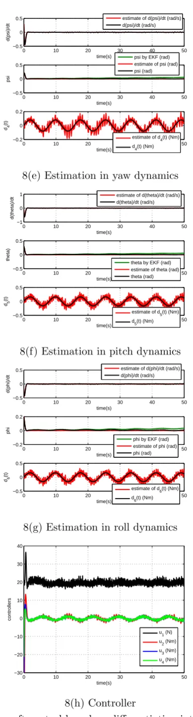
8(e) Estimation in yaw dynamics

0 10 20 30 40 50

−1 0 1

time(s)

d(theta)/dt

estimate of d(theta)/dt (rad/s) d(theta)/dt (rad/s)

0 10 20 30 40 50

−0.5 0 0.5

time(s)

theta)

theta by EKF (rad) estimate of theta (rad) theta (rad)

0 10 20 30 40 50

−0.5 0 0.5

time(s)

d5

(t)

estimate of d

5(t) (Nm)

d

5(t) (Nm)

8(f) Estimation in pitch dynamics

0 10 20 30 40 50

−0.5 0 0.5

time(s)

d(phi)/dt

estimate of d(phi)/dt (rad/s) d(phi)/dt (rad/s)

0 10 20 30 40 50

−0.2 0 0.2

time(s)

phi

phi by EKF (rad) estimate of phi (rad) phi (rad)

0 10 20 30 40 50

−0.5 0 0.5

time(s)

d6

(t)

estimate of d

6(t) (Nm)

d

6(t) (Nm)

8(g) Estimation in roll dynamics

0 10 20 30 40 50

−30 −20 −10 0 10 20 30 40

time(s)

controllers

u

1 (N)

u₂ (Nm) u₃ (Nm) u

4 (Nm)

8(h) Controller

−20 0 20 −20 −10 0 10 20 0 10 20 30 40 x (m) y (m) z (m) Desired trajectory actual trajectory estimate trajectory

9(a) Position trajectory

0 200 400 600 800 1000

−0.5 0 0.5

time(s)

x1

estimate of x

1 (m)

x

1 (m)

x

d (m)

0 200 400 600 800 1000

−2 0 2

time(s)

x2

estimate of x

2 (m/s)

x

2 (m/s)

dx

d/dt (m/s)

0 200 400 600 800 1000

−2 0 2 time(s) d1 (t)

estimate error of d

1(t) (N)

9(b) Estimation in x coordinate

0 200 400 600 800 1000

−0.5 0 0.5

time(s)

y1

estimate of y

1 (m)

y₁ (m) y

d (m)

0 200 400 600 800 1000

−2 0 2

time(s)

y2

estimate of y

2 (m/s)

y

2 (m/s)

dy

d/dt (m/s)

0 200 400 600 800 1000

−1 0 1 time(s) d2 (t)

estimate error of d

2(t) (N)

9(c) Estimation in y coordinate

0 200 400 600 800 1000

−50 0 50

time(s)

z1 estimate of z₁ (m)

z

1 (m)

z

d (m)

0 200 400 600 800 1000

−5 0 5

time(s)

z2

estimate of z

2 (m/s)

z

2 (m/s)

dz_d/dt (m/s)

0 200 400 600 800 1000

−2 0 2 time(s) d3 (t

estimate error of d₃(t) (N)

0 200 400 600 800 1000 −0.5

0 0.5

time(s)

d(psi)/dt

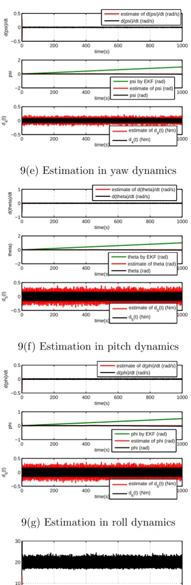
estimate of d(psi)/dt (rad/s) d(psi)/dt (rad/s)

0 200 400 600 800 1000

−2 0 2

time(s)

psi

psi by EKF (rad) estimate of psi (rad) psi (rad)

0 200 400 600 800 1000

−0.5 0 0.5

time(s)

d4

(t)

estimate of d

4(t) (Nm)

d

4(t) (Nm)

9(e) Estimation in yaw dynamics

0 200 400 600 800 1000

−1 0 1

time(s)

d(theta)/dt

estimate of d(theta)/dt (rad/s) d(theta)/dt (rad/s)

0 200 400 600 800 1000

−2 0 2

time(s)

theta) _{theta by EKF (rad)}

estimate of theta (rad) theta (rad)

0 200 400 600 800 1000

−0.5 0 0.5

time(s)

d5

(t)

estimate of d

5(t) (Nm)

d

5(t) (Nm)

9(f) Estimation in pitch dynamics

0 200 400 600 800 1000

−0.5 0 0.5

time(s)

d(phi)/dt

estimate of d(phi)/dt (rad/s) d(phi)/dt (rad/s)

0 200 400 600 800 1000

−1 0 1

time(s)

phi

phi by EKF (rad) estimate of phi (rad) phi (rad)

0 200 400 600 800 1000

−0.5 0 0.5

time(s)

d6

(t)

estimate of d

6(t) (Nm)

d

6(t) (Nm)

9(g) Estimation in roll dynamics

0 200 400 600 800 1000

−30 −20 −10 0 10 20 30

time(s)

controllers

u

1 (N)

u

2 (Nm)

u₃ (Nm) u

4 (Nm)

9(h) Controller

The position measurement outputs are yopi=wi,1+ni, wherei= 1,2,3, andw1,1 =x,w2,1=y,

w3,1 = z; the attitude measurement outputs are yopi = wi,2+ni, wherei= 4,5,6, and w4,2 = ˙ψ,

w5,2= ˙θ,w6,2 = ˙ϕ;ni (wherei= 1,· · · ,6) are the disturbances.

The disturbances ni (where i = 1,· · · ,6) include two types of noises: Random number with

Mean=0, Variance=0.001, Initial speed=0, and Sample time=0; Pulses with Amplitude=0.001, Period=1s, Pulse width=1, and Phase delay=0.

The parameters of the aircraft control system are given as follows:

Quadrotor aircraft [29]: m= 2kg,g= 9.81m/s2,l= 0.2m,Jx = 1.25N s2/rad,Jy = 1.25N s2/rad,

Jz = 2.5N m; b = 2.923×10−3, k = 5×10−4, kx = ky = kz = 0.01N s/m, kψ = kθ = kϕ =

0.012N s/rad;

Third-order differentiator: ki,1= 6, ki,2 = 11,ki,3= 6, i= 1,2,3;

In order to reduce the peaking phenomena in the outputs of the differentiator due to the large

initial observation errors, the perturbation parameters are selected as 1/εi=

{

5t, t≤1

5, t >1 , i= 1,2,3;

Differentiation-integration observer: k2,i,1 = 0.1,k2,i,2 = 2,k2,i,3= 1, i= 4,5,6;

Because the initial observation errors are small for the differentiation-integration observer, no chattering phenomenon happen, and the perturbation parameter can be selected as εi = 1/3,

i= 4,5,6;

Reference trajectory: h0= 30m,a= 5m/s2,km= 0.005;

Controllers: kp1= 16, kp2 = 8,ka1 = 28, ka2 = 8.

In this simulation, without the information of velocity, attitude angle and uncertainties, the air-craft is controlled to track the reference trajectory. The position is obtained from the GPS receiver, and the altitude information is from the altimeter. The angular velocity ( ˙ψ,θ,˙ ϕ˙) is measured by the IMU. Differentiation-integration observer (50) is used to estimate the attitude angle (ψ, θ, ϕ) and uncertainties in the attitude dynamics from measurement of the angular velocity ( ˙ψ,θ,˙ ϕ˙). The third-order differentiator (48) is adopted to estimate the velocity ( ˙x,y,˙ z˙) and uncertainties in the position dynamics from the measurement of position (x, y, z). Controllers (56) and (59) are designed to control the aircraft to track the reference trajectory.

The data of flying test are presented in Figs.8 and 9. Fig. 8(a) describes the position trajectory; Fig. 8(b) describes the estimate ofx,dx/dtand d1(t); Fig. 8(c) describes the estimate of y,dy/dt

and d2(t); Fig. 8(d) presents the estimate ofz,dz/dt and d3(t); Fig. 8(e) presents the estimate of

the yaw angleψ, yaw ratedψ/dtandd4(t); Fig. 8(f) presents the estimate of the pitch angleθ, pitch

rate dψ/dt andd5(t); Fig. 8(g) presents the estimate of the roll angle ϕ, roll rate dϕ/dtand d1(t);

Fig. 8(h) presents the controller curves ofu1,u2,u3andu4. The simulation in 1000s is proposed in