Pushed and pulled fronts in a discrete reaction diffusion equation

Pushed and pulled fronts in a discrete reaction-diffusion

equation

J.R. King & R.D. O’Dea

Centre for Mathematical Medicine and Biology,

School of Mathematical Sciences,

University of Nottingham, University Park,

Nottingham, NG7 2RD, UK

September 25, 2015

Abstract

We consider the propagation of wave fronts connecting unstable and stable uniform solutions to a discrete reaction-diffusion equation on a one-dimensional integer lattice. The dependence of the wavespeed on the coupling strengthµbetween lattice points and on a detuning parameter (a) appearing in a nonlinear forcing is investigated thoroughly. Via asymptotic and numerical studies, the speed both of ‘pulled’ fronts (whereby the wavespeed can be characterised by the linear behaviour at the leading edge of the wave) and of ‘pushed’ fronts (for which the nonlinear dynamics of the entire front determine the wavespeed) is investigated in detail. The asymp-totic and numerical techniques employed complement each other in highlighting the transition between pushed and pulled fronts under variations ofµanda.

1

Introduction

Mathematical analyses of a wide variety of physical and biological systems lead to investigation of spatially-discrete nonlinear reaction-diffusion equations of the form

duj

dt =µ(uj+1−2uj+uj−1) +f(uj;a), (1)

on a discrete integer lattice with lattice points j ∈ Z _{at which uj = uj(t), the parameter µ >0}

dictating the coupling strength between lattice points while the constantaparameterises the non-linearity (see below). Such models arise in, for example, the study of crystal growth [1] and binary alloy evolution [2] in material science and of neural networks for image processing and pattern recog-nition [3, 4]; additionally, analogous formulations emerge naturally in the study of cell population growth [5] and cell signalling [6–9]. Lastly, such systems of course occur in the numerical solution by spatial discretisation of partial differential equations. We remark, however, that the formulations investigated in the above studies, and the equation analysed herein, are to be viewed as truly spa-tially discrete, and not as discretised versions of PDEs; indeed, the results that we present serve to illustrate how the behaviour of the continuous analogue of (1) relates to that of the discrete system, representing one of the simplest systems in which such a discrete-to-continuous transition can be explored.

discrete models and their continuous counterparts. Here, however, our focus is on the propagation of heteroclinic connections between unstable and stable states (rather than stable–stable connections), for which travelling wave solutions to the continuous Fisher (or Kolmogorov-Petrovskii-Piskunov (KPP)) equation, in particular, have been extremely widely studied. In the discrete case, Zinner et al. [17] considered the existence of travelling-wave solutions to the discrete Fisher-KPP equation on a one-dimensional lattice, obtaining a constraint on the coupling strength for which strictly increasing travelling wavefronts of speedc >0 exist; more recent work on related systems includes that of Guo and Morita [18] and Hakberg [19].

In this study, we consider for definiteness (and because of its widespread adoption as a model nonlinearity in the PDE case) equation (1) with the following cubic nonlinearity

f(u;a) =u(1−u)1 + u

a

, (2)

and investigate the dependence on the parametersµand aof the wave propagation speed through a discrete lattice. We emphasise that the specific form (2) is adopted for illustrative purposes; the features that we analyse below are applicable to a broad class of nonlinearities and much of the analysis applies to more general cases of smoothf with (1) scaled such that

f(u;a) =u+o(1) asu→0, f(1;a) = 0, f(u;a)>0 for 0< u <1. (3) The parameter a > 0 is often termed the ‘detuning parameter’ in the literature (e.g. Cahn et al. [13]). The uniform steady state solutions of (1), (2) areuj ≡0 (unstable) and uj ≡1,−a(stable

for a >0). We remark that (1), (2) contains as limit cases both the (monostable) discrete Fisher

equation (a→ ∞), with steady statesuj ≡0,1, and the (bistable) discrete Newell-Whitehead-Segel equation with stable states uj ≡ ±1 (a = 1). Our interest here will be in fronts in which the stable state uj = 1 overruns the unstable one uj = 0. In the continuous counterpart of equation (1),µcorresponds to the diffusion coefficient; the study of travelling wave fronts in such continuous diffusion equations with a range of choices for the nonlinearity f(u;a) has been the subject of extensive investigation, in a wide variety of contexts, including (but not limited to) mathematical biology, plasma dynamics and pattern formation. We do not give a thorough review here, since our main focus is on the discrete equation; instead, we include a summary of the results of most relevance to the current work in§2.

The emphasis of this work is to characterise, for the first time, the transition that occurs between so-called ‘pulled’ (where the propagation speed, denoted c∗_{, is characterised by the leading-edge}

behaviour) and ‘pushed’ (the entire nonlinear wave profile determines the wavespeed, c†_{) fronts as}

the parametersµandaare varied. While equivalent results are available for the continuum version of (1), (2), we are not aware of previous detailed analysis in discrete equations. Our results may be summarised briefly as follows. Forµ =O(1), c∗_{(µ) is straightforward to obtain; however, neither}

the transitionaT(µ) norc†(a, µ) are available analytically. In the limit a→ 0+, we obtain a new estimate for c†_{(a, µ). For µ≪1, we isolate the transition as aT(µ)∼1/ln(1/µ) and provide new}

results for c†_{(a, µ) (a = O(µ)) and c}† _{and c}∗ _{at transition. The applicability of these results is}

illustrated by comparison with numerical simulation, and with the more well-known results that pertain forµ≫1.

There is an issue that needs setting to one side before proceeding with the detailed analysis: we concern ourselves only with initial data that decay sufficiently rapidly that the minimum wavespeed (denoted henceforth by cmin) of strictly positive travelling waves is realised. To characterise what ‘sufficiently rapidly’ means here, we note that (1), (3) linearised about u = 0 has travelling-wave solutionsuj= exp(−λ(j−ct)), with

λc= 2µ(cosh(λ)−1) + 1. (4)

Hencec(λ) takes its minimum value when

c= 2µsinh(λ) (5)

and (4) both hold. When the initial data behave as exp(−λj) asj→+∞, whereλis less than the value determined by (4), (5) and the resultingc given by (4) has c > cmin, then that value ofc is realised as the large-time behaviour; for more rapidly decaying initial data we are in the territory analysed in the remainder of the paper.

The paper is organised as follows. In§2 we outline the two distinct classes (pulled and pushed) of waves of relevance here, and analyse the continuum (strong-coupling) limit µ→+∞. In §3 we set up the corresponding discrete travelling-wave problem and in §4, an asymptotic analysis of the transition between pulled and pushed waves in (1) is performed. §5 considers the weak-coupling limit (µ → 0+_{) in detail. In §6, we present numerical simulations indicating the key features of} travelling wave behaviour, and illustrating the applicability of the asymptotic results derived in previous sections. §7 includes a summary of the main results of this paper. Appendix A addresses the limit a→0+_{, Appendix B treats a linear differential-difference equation crucial to the results} of §5, Appendix C gives an analysis of both stable–unstable and stable–stable connections for the case of a specific (explicitly solvable) nonlinear coupling between lattice points and Appendix D generalises aspects of the analysis of§2 and§4 to a much broader setting.

2

Pushed and pulled fronts and the continuum limit

µ

_→

+

_∞

This paper focusses on the propagation speed of large-time (travelling-wave) solutions to equations (1), (2) in a one-dimensional integer latticej∈Z_{on whichuj=uj(t). We consider in particular how}

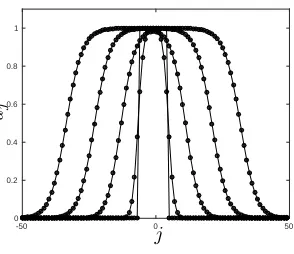
these speeds differ from those obtained in the corresponding continuous reaction-diffusion equation. The type of behaviour with which we are concerned is illustrated in Figure 1, which shows a nu-merical solution indicating the evolution to two travelling waves (one propagating in each direction) from initial data given by (see§6 for details of the numerical procedures adopted)

uj(0) =

(

1, −56j65,

0, otherwise. (6)

Our analysis will concern the rightward travelling wave, the other following from an obvious sym-metry argument.

Stable-unstable connections in systems such as (1) may be categorised into two distinct classes: in the case for which the propagation speed is determined by the leading edge of the wave, the front is termed ‘pulled’; conversely, in the case of ‘pushed’ waves, the wavespeed is determined by the whole of the wavefront1_{. The pulled speed can be obtained by linearising the system around the} homogeneous state (and is therefore also frequently referred to as the ‘linearly-selected’ wavespeed); in this regime, the unstable homogeneous state is invaded by the stable one at a speed which tends to a constantc∗ _{as t→ +∞; when nonlinear effects are dominant in a sense that will be clarified}

below, invading waves of speedc† _{> c}∗ _{are obtained, and in such circumstances the linear analysis}

provides a lower bound for the pushed speed, but does not give the realised speed. Determining the

1_{An early description of the distinct classes of wave in reaction-diffusion equations of the form (7) was given by}

-50 0 50 0

0.2 0.4 0.6 0.8 1

j uj

Figure 1: Numerical solution to (1), (2) for µ = 10, a = 0.5, at times t = 0,0.15,1.75,3.5,5.25 indicating propagating front behaviour from an initial state given by (6).

class of wavefronts exhibited by a given discrete system is, in general, difficult (see,e.g., Plahte and Øyehaug [8]); in the continuous case (with a monostable nonlinearity), approaches to achieve this include that of Lucia et al. [22], but such methods do not seem likely to be applicable in the discrete case.

In the limit µ → +∞ in (1), neighbouring lattice points have (after an initial transient t =

O(1/µ), unless the initial data are suitably prepared) almost equal values ofuj,i.e. the solution is slowly varying with respect toj. The appropriate spatial variable isx=j/√µ; under this rescaling, withuj(t)∼u(x, t), we obtain

∂u

∂t =

∂2u

∂x2+f(u;a). (7)

Since the seminal studies of Fisher [23] and Kolmogorov et al. [24], travelling wave solutions to (7) have been widely investigated; see,e.g., the review of van Saarloos [25].

Travelling-wave solutions of (7) take the formu(x, t)∼U(z),z=x−S(t),S(t)∼ctfor constant2

c and satisfying

U′′_+cU′_{+f(U;a) = 0, (8)}

U →1, z → −∞; U →0, z →+∞. (9)

These describe the heteroclinic connections between the stable state u = 1 and the unstable one

u= 0; note that for givenc >0, (8), (9) should be viewed as an initial value problem fromz=−∞, the solution then being determined up to translations in z. Linearising (8) as z → +∞ gives (in view of (3))

U′′_+cU′_{+U= 0, (10)}

so that

U =A₋e−(c₋√c2

−4 )z/2_+A+e−(c+√c2

−4 )z/2_{, c}

6

= 2. (11)

Positivity (required by the comparison theorem for non-negative initial data) thus requires c>2. In the phase plane of (8), the origin is a degenerate stable node ifc= 2, in which case (10) implies

U = e−z_{(Az+B) (12)}

and, when A >0 holds for the solution to (8), (9), c= 2 is the wavespeed associated with a pulled front (i.e. c∗_{= 2). Asadecreases (in the case of (2), and more generally in (1), (3) ifais suitably}

defined), A reaches zero at a= aT, say, and for smaller a with 2 < c < c† for some c†(a), U(z) in (10) becomes negative at somez, approaching zero from below as z →+∞ (as can readily be demonstrated by a phase-plane analysis, a method that is not of course available in the discrete

2_{Due to the rescaling ofjthe constantcin the remainder of this section corresponds to dividing that elsewhere in}

case); such non-monotonic waves are unstable and are in any case again precluded for non-negative initial data by the comparison theorem. In this case, pushed fronts occur and we now further classify the two cases (summarising well-known results for (7)), wherebycmin=c∗ fora > aT (pulled front)

andcmin=c†(a)> c∗ for 0< a < aT (pushed front).

(a) Pulled fronts: a > aT, cmin = 2. The wavespeed here follows either via (12) from the

linearisation (10) of the travelling-wave ODE or from an application of the Liouville-Green (JWKB) method to the linearised PDE

∂u

∂t =

∂2_u

∂x2 +u (13)

(cf.Cuesta and King [26] and references therein), whereby

u∼e−φ(x,t)_{, φ(x, t)}

∼tF(x/t) ast→ ∞, x=O(t) (14) gives (sinceφxxdoes not contribute at leading order)

∂φ

∂t +

_∂φ

∂x

2

+ 1 = 0, F −ηdF

dη +

_dF

dη

2

+ 1 = 0, (15)

whereη=x/t. We therefore obtain

F(η) = 1

4η 2

−1, (16)

giving the point at which linearisation becomes inapplicable (i.e. at which the solution (14) fails to be exponentially small) asη = 2 (implyingS(t)∼2t), thereby identifying the nonlinear wavefront as havingc= 2.

(b) Pushed fronts: 0< a < aT,cmin =c†(a). Here the wavespeed is determined by the solution

to (8) having A₋ = 0, A+ > 0 in (11), i.e. fast decay into the origin (the phase-plane analysis demonstrates that fora < aT this is the borderline between thosecfor whichU(z) remains positive and those for which it crosses zero, whereas for a > aT this borderline is given by the degenerate-stable-node case (12)). Fora < aT, the wavespeedcmincan therefore be viewed as an eigenvalue (or second-kind similarity exponent), as is the wavespeed in the case of stable–stable connections; such an interpretation is not appropriate for pulled fronts. Fora=aT we havecmin= 2, the value ofaT being determined via the requirement thatA= 0,B >0 in (12),i.e.in this transition casearather thanccan be viewed as an eigenvalue.

A specific reason for the choice of the nonlinearity (2) is that c† _{can be determined explicitly.}

SettingU = 1/V in (8) gives the quadratically nonlinear ODE

V V′′_−2V′2_{+cV V′}

−(V −1)

V +1

a

= 0 (17)

and established approaches to such problems suggest seeking a solution of the form

V = 1 + eλz (18)

(the solution seems to have been identified for the first time by Hadeler and Rothe [20], without ex-plicitly exploiting the quadratically nonlinear form). Equation (17) leads to two algebraic equations, thereby prescribingcas well asλ, namely

λ2−cλ+ 1 = 0, λ2+cλ−1−1_a= 0, (19) so that

λ= 1/√2a, c= 1/√2a+√2a. (20)

Thus, in (11) we have

1 2

c+pc2₋₄₌

(√

2a fora >1/2

and conversely for the negative square root. Hence (18), (20) corresponds to fast decay fora <1/2 but slow decay for a >1/2 (the latter will pertain for initial data that decay as exp −x/√2a

as

x→+∞). We thus conclude that

aT = 1/2, c†(a) = 1/

√

2a+√2a (22)

and we note that

c†(1/2) = 2, dc†

da(1/2) = 0, (23)

implying thatcmin(a) behaves rather smoothly asapasses throughaT (cf.§4). In summary, for (7) we have

cmin(a) =

(

1/√2a+√2a, 0< a61/2,

2, a>1/2, (24)

(the latter in fact also holds for a <−1, but we shall limit ourselves to a >0). For more general nonlinearities (3), cmin = 2 for a > aT remains true but c†(a) and aT each need determining numerically.

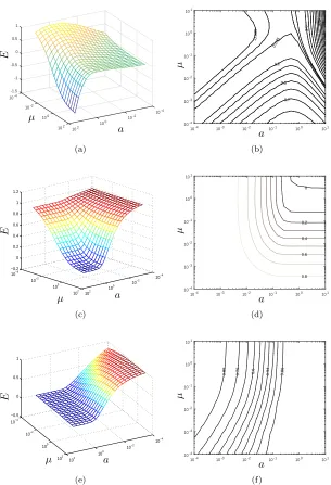
The surface and contour plots in Figure 2 illustrate the range of applicability (by comparison with numerical simulations of (1); see §6 for details of the numerical procedures employed) of the above results in (µ, a) parameter space, namely the continuum wavespeeds (24) (rescaled by√µ, as required for comparison with the discrete problem), appropriate for largeµ (each in its own range ofa– see§7), and the pulled speed determined by (4), (5), appropriate fora > aT(µ).

3

Travelling wave analysis of the discrete system

We now set3

uj(t)∼U(z), z =j−S(t), S(t)∼ctast→+∞ (25)

in (1) to give the ordinary-differential-difference equation

µ(U(z+ 1)−2U(z) +U(z−1)) +cdU(z)

dz +f(U(z);a) = 0, (26)

U→1 asz→ −∞; U →0 asz→+∞. (27)

We note that while (1) holds for j∈Z_{, (26) applies forz∈}R_{, in keeping witht ∈}R+ _{applying in}

(1). Unlike the continuous case, this cannot be treated as an initial value problem from z=−∞; a boundary-condition count (respecting the invariance of (26) under translations ofz) implies that (for given c) the required degrees of freedom as z → +∞ (of the form exp(−λz)) involve all the roots of (4) having positive real part. Pulled fronts havec∗_{(µ) and λ}∗_{(µ) given by (4), (5) with}

λ∗ _{real, (5) being the repeated-root condition (cf.Zinner et al. [17], equation (6), the supremum in}

which is related to the minimum wavespeed statement that led to (5) above); (4) has two real roots

forc > c∗ _{>0 (these also being its roots with the smallest positive real part) and none forc < c}∗_.

Pushed fronts are those for whichf(u;a) is such that there is ac=c†_{> c}∗_{for which the exponential}

corresponding to the smaller positive real root of (4) is absent asz→+∞in the solution to (26), (27) (i.e. fast decay occurs).

From (4), (5) we have thatλ∗_(µ),c∗_{(µ) are given by}

2µ(cosh(λ∗_)−λ∗_sinh(λ∗_{)−1) + 1 = 0, c}∗_{= 2µsinh(λ}∗_{). (28)}

This implies

λ∗_(µ)∼√1

µ

1−₈1_µ

, c∗_(µ)∼2√_µ

1 + 1 2µ

as µ→+∞, (29)

3_{We stress that, becausex=j/}√_{µ, the quantitiesz,S,candλhenceforth are scaled differently from those in the}

10-4 10-2 100 102 102 100 10-2 -0.5 0 -1 0.5 1 -1.5 10-4 E µ a (a) 0.035 -0.035 -0.2 0.5 0.2 0.7 -0.9

10-4 10-3 10-2 10-1 100 101 10-4 10-3 10-2 10-1 100 101 µ a (b) 10−4 10−2 100 102 10−4 10−2 100 102 −0.2 0 0.2 0.4 0.6 0.8 1 1.2 E µ a (c) 0.2 0.4 0.6 0.8 0

10-4 10-3 10-2 10-1 100 101 10-4 10-3 10-2 10-1 100 101 µ a (d) 10−4 10−2 100 102 10−4 10−2 100 102 −0.5 0 0.5 1 E µ a (e) 0.06 0.34 0.6 0.79 0.88

10-4 10-3 10-2 10-1 100 101 10-4 10-3 10-2 10-1 100 101 µ a (f)

Figure 2: Surface (a,c,e) and contour (b,d,f) plots showing the relative deviation of the propagation speedcobserved in (time-dependent) numerical simulations of (1) from the results (4), (5) and (24):

the leading orders in which are consistent with the results of the previous section; forµ →0+ _we haveλ∗_→+∞and

µ(λ∗_−1)eλ∗

∼1, c∗_∼µeλ∗

, (30)

with only terms exponentially smaller inλ∗ _{neglected, so that asµ→0}+_,

λ∗_{∼ln(1/µ)−ln ln(1/µ) +}ln ln(1/µ)

ln(1/µ) + 1

ln(1/µ), c∗∼ 1 ln(1/µ)+

ln ln(1/µ) ln2(1/µ) +

1

ln2(1/µ). (31)

These logarithmic dependencies provide advanced warning of the asymptotic challenges that will arise in§5.4.

In the discrete case we have been unable to identify any f(u;a) for whichc† _{can be determined}

explicitly for a pushed front (a somewhat abortive attempt to generalise (17) in this direction, ex-ploiting a corresponding quadratically nonlinear form, is given in Appendix C); explicit solutions can be constructed by specifying a suitable specific profile forU(z) and then determining the non-linearityf from (26), but the resultingf will in general then depend onµ, so this procedure is not suitable for the current purposes. For example, proceeding in this way we find that for

f(u;a, µ) = u(1−u) (1 +u/a+ (1 + 1/2a)u(1−u)/2aµ)

1 +u(1−u)/2aµ (32)

the ansatz

U(z) = 1

1 + eλz (33)

again applies withλandcgiven by

2µ(cosh(λ)−1) = 1/2a, cλ= 1 + 1/2a; (34) however, the dependence of (32) uponµmakes it of limited value to the current study.

4

Asymptotic analysis of the transition between pushed and

pulled fronts

In this section we analyse the behaviour close to the transition between pushed and pulled fronts – while we shall do so here in the framework of the ordinary-differential-difference equation (26), the criteria in question are of much more general applicability: see Appendix D. In the current context the analysis of this section will provide a diagnostic that is helpful in the analysis of the weak-coupling limitµ→0+_.

We require the solution to (26), defined uniquely for given wavespeedc up to translations inz

– an indeterminacy that we shall eliminate by specifying U(0) = 1/2 – and (as usual) determine c

through the requirements thatU >0 forz∈(−∞,∞) and thatU(z) exhibits a maximal decay rate asz→+∞.

We denote the two real roots of (4) withc > c∗_byλ+andλ

−, withλ+> λ₋. Pushed fronts have

U(z) decaying as exp(−λ+z) asz→+∞withλ+=λ†> λ∗, λ†(a, µ) andc†(a, µ) being related by (4). It is immediate from (4) and (5) that

c(λ)∼c∗₊µcosh(λ∗)

λ∗ (λ−λ∗)

2_{as λ→λ}∗_{, (35)}

i.e.

λ_±∼λ∗±

s

λ∗

µcosh(λ∗₎(c−c∗) asc→c

∗+_{. (36)}

For pulled fronts, having c =c∗_{(µ), we denote U =U}∗_{(z;a). We reiterate that we denote by}

generality4_{) and pushed fronts (a < a}

T) occurs. Then fora6=aT we have (cf.(12))5

U∗_{(z;a)∼(A(a)z+B(a)) e}−λ∗_z

asz→+∞, (37)

the z prefactor being associated with λ = λ∗ _{being a repeated root. In (37) we have A > 0 for}

a > aT andA <0 fora < aT. While only the former is realisable for non-negative initial data,U∗

will also play a role in the sequel fora < aT. At the transition, we have (cf. Cuesta and King [26])

U∗_(z;aT)∼BTe−λ∗_z

asz→+∞, (38)

in whichBT =B(aT)>0 andA(aT) = 0. Conversely, forc > c∗, we have fora6=aT

U(z;a)∼A₋(a, c)e−λ−(c)z asz→+∞, (39)

withA₋(a, c)>0 fora > aT and fora < aT withc > c†(a, µ);A−(a, c)<0 holds fora < aT with6

c∗_{(µ)< c < c}†_{(a, µ), as doesA}

−(a, c†) = 0 fora < aT in which case

U†_(z;a)∼A†

+(a)e−λ+z asz→+∞ (40)

withA†+>0, and whereU†(z;a) denotes the pushed front profile7, having propagation speedc†. The key implications of the above analysis for the current section are as follows. Setinga=aT+δ with|δ| ≪1 we have from (37) that forδ >0

U∗(z;a)∼(BT +δB′(aT) +δA′(aT)z)e−λ

∗_z

as δ→0+, z→+∞ (41) while forδ <0 it follows from (40) that8_{, retaining terms up toO(δ),}

U†(z;a)∼A+†(aT) +δA†′+(aT)

(1−(λ+−λ∗)z) e−λ

∗_z

, (42)

asλ∗_{→λ+,z→+∞(as we shall see in (46), λ+−λ}∗_=O(δ)).

Now, returning to (26), we set

U(z)∼U0(z) +δU1(z) +δ2U2(z), c∼c∗_+δ2_{C, (43)}

asδ→0, and it follows that

U0(z) =U∗(z;aT), U1(z) = ∂

∂aU

∗_(z;a

T) (44)

in both the pulled (δ >0) and pushed (δ <0) cases. In view of (38), the matching condition (41) is automatically satisfied, while in (42) we infer from (35)–(36) that

A†+(aT) =BT, A+†′(aT) =B′(aT), (45)

λ+−λ∗∼ −

δ

BT

A′_(a

T), C=

µcoshλ∗

λ∗

_A′(a

T)

BT

2

, (46)

asδ→0−_{. Thus}

c†(a, µ)∼c∗(a) + (aT −a)2C, asa→a−_T (47) expresses the rather smooth transition ofcmin(a, µ) throughaT.

4_{Provided – as in the case of the cubic nonlinearity on which we mainly focus – only one such transition occurs; a}

characterisation of the nonlinearitiesf(u;a) in such regards would be valuable.

5

We suppress the dependence ofUonµin our far-field expressions.

6_{Note thatc}†_(a

T, µ) =c∗(µ).

7

The far-field expansion (39) will also in general contain a contribution of the form (40) withA†+ replaced by

A+(a, c), withA†+(a) =A+(a, c†).

5

The weak-coupling limit,

µ

_→

0

5.1

Na¨ıve time-dependent analysis

For reasons of notational convention, we set µ =ε in this section, and consider the behaviour of propagating fronts in (26), (27) for 0< ε≪1. It should be clear how the nonlinearityf(u;a) could be generalised; we shall again limit ourselves to the cubic form defined by (2).

Returning to the notationuj(t), consider, for definiteness, the following initial data:

uj(0) = 1, j60, uj(0) = 0, j >0. (48)

Thenuj∼1 forj60 holds asε→0 for all time, and setting uj∼εjvj forj >0,t=O(1) gives dv1

dt = 1 +v1,

dvj

dt =vj−1+vj, j>1, (49)

and so

v1= et−1, vj= (−1)j 1−et

j₋1

X

m=0 (−1)mt

m

m!

!

. (50)

Thusu1 becomes ofO(1) on the timescale t1=O(1), where

t= ln(1/ε) +t1, (51)

with leading order balance9

du1 dt1

=u1(1−u1)(1 +u1/a), (52)

withu1∼et1 ast1→ −∞, and henceu1(t1) is given by

ln(u1)−_{a+ 1}a ln(1−u1)−_{a+ 1}1 ln(1 +u1/a) =t1. (53)

In (50), the final term in the summation dominates fort≫j, so application of Stirling’s formula gives

uj∼ ε

j_et_tj−1

√

2πjjj−1_e−j,fort≫j≫1. (54) Settingj =ct, it is required for (54) to be ofO(1) that

c(ln(1/ε) + ln(c)−1)∼1, (55)

which corresponds exactly to eliminatingλ∗ _{in (30), as might be expected.}

Subsequent lattice points (j >1) are activated on timescalestj =O(1), where

t=Tj(ε) ln(1/ε) +tj, Tj(0) =j, (56)

from which the wavespeed will be inferred viac(ε) =j/Tj(ε) ln(1/ε); then

duj dtj

=uj(1−uj)(1 +uj/a), (57)

and10_u

j ∼etj astj→ −∞, so thatuj =u1(tj). That the I.V.P. (57) is identical to (52) corresponds to the solutions approaching a waveform of fixed profile and wavespeed

c∼1/ln (1/ε) asε→0+. (58)

9_{Here we assumea=O(1); the behaviour differs significantly fora=O(ε) – see}

§5.3 below.

10_{Setting the coefficient of the exponential to unity in the initial condition requires appropriate choice of the}

Thus, once activated, each lattice point in turn activates its neighbour after a fixed timestep ∆t∼

ln (1/ε), corresponding to a simple cellular automaton. The analysis above gives little insight into whether the mechanism of wavespeed selection is of pulled or pushed type (even though (55) has the same asymptotic behaviour asc∗_{(ε)). For example, (49) is independent of the nonlinearity while}

(57) is not; more substantially, the use above of (49) (the linearised behaviour ahead of the front) is consistent with pulled behaviour (and we shall find that this indeed occurs fora=O(1)), whereas the discrete-time and two-state (uj = 0 oruj = 1) cellular automaton just referred to would have

uj ≡0 ahead of the wavefront, which might be interpreted as requiring pushed behaviour (which will arise below for alogarithmically small inε). The transition between pulled and pushed fronts proves delicate to analyse and is therefore treated in some detail below (see§5.4).

5.2

Travelling-wave preliminaries

We now consider in more detail the small-µasymptotics of travelling waves in the system (26), and their propagation speed. From (4), withµreplaced byε, it follows that forc=O(1) the real roots

λ+> λ− have

λ₋∼1/c, λ+∼ln (1/ε), (59)

so the faster decaying case, at least, exhibits very rapid decay inzin the limitε→0.

It will prove useful in the sequel to introduce the slowness s= 1/cand the distinguished limit that includes the repeated-root (pulled-front) case corresponds toσ=O(1), where

σ=εses, (60)

i.e.

s∼ln(1/ε)−ln (ln(1/ε)) + ln(σ). (61) Sinceλ_± are both large in this regime, (4) can be approximated (to all orders in ln(1/ε)) by

εeλ∼λc−1, (62)

i.e., setting λ=s+ Λ,

σeΛ∼Λ, (63)

the repeated-root case (5) having Λ∼1,σ∼1/e.

We now discuss the travelling-wave behaviour in the two regimes implicitly identified above, namely (i) a pushed case,c†_{=O(1) and (ii)σ=O(1), the former being significantly simpler but of}

less import for our purposes, in the sense that it resides firmly in the pushed-front regime.

5.3

a

=

O

(

ε

)

Pushed fronts withc† _{=O(1) havea=O(ε). Here we first analyse an inner problem, which involves}

settinga=ε/αandz=εc†_{ξto give at leading order forξ=O(1)}

dU0 dξ +αU

2

0(1−U0) = 0, (64)

with U0 →1 as ξ → −∞, U0 →0 as ξ→+∞, andU0(0) = 1/2. On straightforward integration, the solution may be obtained in implicit form as

1

U0 −ln

_U

0 1−U0

=αξ+ 2 (65)

with limiting behaviour

U0∼1/αξasξ→+∞. (66)

The outer scaling setsz=c†_{ζ, U =εV whereby}11

dV0

dζ +V0(1 +αV0) = (

−1 0< ζ < s

0 ζ > s (67)

and, as ζ → 0+_{, V}

0 ∼ 1/αζ. The solution to (67) decays as e−ζ as ζ → ∞ for almost all s, corresponding to first of (59). To obtain a pushed front we thus require thats be determined such that the leading-order solution satisfies

V0= 0 atζ=s, V0≡0 forζ > s. (68) Hence

V0=

     1 2α √

4α−1 cot (√4α−1)ζ/2

−1

, α >1/4;

4

ζ −2, α= 1/4;

1 2α

√

1−4αcoth (√1−4α)ζ/2

−1

, α <1/4,

(69)

so that

s(α)∼

     2 √_4α −1tan−

1 √_4α

−1

, α >1/4;

2, α= 1/4;

2

√

1−4αtanh

−1 √₁

−4α

, α <1/4,

(70)

thereby providing explicitly the pushed speed (viac = 1/s) in terms of the detuning parameter in this regime (recall,a=ε/α).

Asα→+∞we have

V0∼√1

αcot(

√

αζ), s∼₂√π

α, c

†_∼ 2 √

α

π , (71)

this limit corresponding to the case in which the nonlinearity is quadratic, rather than linear, as

u→0, in which case it is trivially clear that the front must be nonlinearly selected (i.e. pushed); see also Appendix A. Asα→0+

V0∼

1

α

e−ζ

1−e−ζ forζ=O(1); V0∼ 1

αe

−ζ_{−1 forζ= ln(1/α) +O(1), (72)}

and

s∼ln(1/α), c†_∼ 1

ln(1/α). (73)

BecauseV =o(1) forζ > s, describing the transition to the exponential decay associated withλ+ in (59) requires significantly more involved asymptotics, which we shall not pursue. In summary, we have shown here that a pushed front occurs forµ→0+,a=O(ε); settinga=ε/αthe leading-order expressions forc†_{(a, µ) are}

c†(ε/α,0) =

√

1−4α

2

1 tanh−1₍√₁

−4α), α <1/4;

c†(4ε,0) = 1/2, α= 1/4;

c†_{(ε/α,0) =}

√

4α−1 2

1

tan−1₍√_4α−1), α >1/4.

               (74)

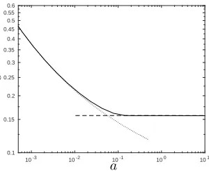
A comparison of these results, and of the pulled ones (4), (5), with the speed observed in numerical simulations of (1), (2) is shown in Figure 3; the agreement is excellent other than in an intermediate range ofathat we address in the next subsection.

11_{The ‘}

10-3 ₁₀-2 ₁₀-1 ₁₀0 ₁₀1

0.1 0.15 0.2 0.25 0.3 0.35 0.4 0.45 0.5 0.55 0.6

a

c

Figure 3: Comparison of wavespeeds obtained from numerical solutions to (1), (2) (solid line) against the pushed estimate (74) (dotted line) and exact pulled speed given by (4), (5), forµ= 10−4_.

5.4

a

=

O

(1)

We shall also in fact cover the regimea=O(1/ln(1/ε)), which proves to be the most important of all, in this subsection. We first consider the pulled case with σ =O(1) in (60). Setting z =c∗_ζ,

with

c∗_∼ 1

ln (1/ε)≪1, s∼ln (1/ε)≫1, (75) (see (61)) gives

ε(U(ζ+s)−2U(ζ) +U(ζ−s)) + d

dζU(ζ) +f(U(ζ);a) = 0. (76)

Hence, setting

U ∼U0(ζ) +εU1(ζ) as ε→0+_{withζ=O(1) (77)}

we have

dU0

dζ +f(U0;a) = 0, U0(0) = 1/2, (78)

so that, for the nonlinearity (2),U0 is given in implicit form by

U0

(1−U0)a/(a+1)_(U

0+a)1/(a+1)

= 1

(1 + 2a)1/(a+1)e−

ζ_{, (79)}

with far-field behaviour

U0∼K(a)e−ζ asζ→+∞, (80)

where

K(a) =

a

1 + 2a

1/(a+1)

. (81)

Moreover,

−2U0+ 1 + dU1

dζ +f′(U0)U1= 0, U1(0) = 0 (82)

so thatU1∼ −1 asζ→+∞.

For z =O(1) with 0< z <1, the contributions for which we need to account follow from the balance (which we continue to write in terms ofζ to make the matching intoζ=O(1) transparent)

ε+dU

dζ +U = 0 (83)

(becauseU(ζ−s)∼1,U(ζ), U(ζ+s)≪1 andf(U;a)∼U) so that

In the remaining regions, the inequalitiesU(ζ+s)≪U(ζ)≪U(ζ−s)≪1 hold, so that

εU(ζ−s) + d

dζU(ζ) +U(ζ) = 0 (85)

provides the relevant balance, and we set12

U(ζ) = e−ζV(z), (86)

to give

d

dzV(z) +σV(z−1) = 0. (87)

We can now appeal directly to the analysis of Appendix B, which is devoted to (87) withz=ξ+1. The initial data in 0< ξ 61 follow13 _{from (84); adopting (111) with ν = 0 andν =s, and using} (114), we then find that14

V(z)∼ 1

1−λ−

K(a)−ελ−+se

λ−+s

λ−+s

e−λ−z, asz→+∞. (88)

It follows from (110) thatλ₋ <1, while s≫1, so the sign of the coefficient in (88) is determined by that of15 _{(using (60) and (110))}

κ(λ₋;a)≡K(a)−λ_s−. (89)

It remains to use (89), withK(a) defined by (81), to infer the value ofσ. For givenλ₋ (and henceσ), ifκ >0 one has slow decay associated with the initial data having behaviour proportional to exp(−λ₋j) asj → ∞(withλ₋ here given by (4)). It is clear thatκis a decreasing function of

λ₋, the latter being maximal in the repeated-root case,i.e. atλ₋= 1. If κ(1;a)>0, we infer that the front is pulled, with (114) being modified in the obvious way (cf. (37)) due toρ=−1 being a second-order pole whenσ= 1/e; however, ifκ(1;a)<0 the minimum-speed non-negative wave will be that for which

κ(λ₋;a) = 0, (90)

corresponding to the wave being of pushed class. Sinces∼ln(1/ε), the condition (90) requires that

a≪1, and hence, in view of (81),K(a) =a+O(a2_{) and}16 _{a=O(1/ln(1/ε)). Hence, at transition,} we have

aT ∼

1

ln(1/ε) asε→0

+_{, (91)}

and the pushed fronts that occur fora < aT have (using (110))

λ₋ ∼aln (1/ε), σ∼aln (1/ε) e−aln(1/ε) (92) and hence, from (61),

s∼ln(1/ε)−aln(1/ε) + lna. (93)

12_{That the other terms from the central difference operator are negligible in (85) follows from the factors e}−s_arising

from the transformation fromU toV.

13_Becauseζ

≪sin (78), this fully nonlinear region makes no leading-order contribution to the integral in (109), though the contribution it does make is only logarithmically smaller: self-consistency checks incorporating such correction terms have been undertaken to confirm that they do not lead to the expansions derived in this section becoming invalid in the regimes considered.

14_{The notationλ}

−is that of Appendix B, not that above; the two usages ofλ±are in correspondence, however.

15_{It will be clear by now that we are, in the interests of brevity, including in a number of such expressions terms}

that may not be of the same order. We affirm, in line with the footnote before last, that the analysis is nevertheless not ad hoc: that the various terms that contribute to the final conclusions (and only such terms) have each been retained has been subject topost hocanalysis; the linearity of (87) plays an important part in such considerations.

16_{Again, it can be confirmed that the above expressions remain valid at leading order under this scaling,}

so that

c†_{(a, ε)∼} 1

ln(1/ε)+

a

ln(1/ε)− lna

ln2(1/ε). (94)

It is clear from (91) and (93) that, to these orders, ds/da= 0 ata=aT, consistent with the analysis of§4 (recalling thatc= 1/s). Moreover, formally settinga≪1/ln (1/ε) in (93) gives

s∼ln(a/ε), c†_∼ 1

ln(a/ε), (95)

thereby matching successfully with the regime analysed in§5.3 (see (73)).

Much of the analysis of pushed fronts (notably in Appendix B) here relies, unusually, on lin-earisation ahead of the wavefront; the nonlinear profile from (79) feeds through only in the small-a

behaviour ofK(a) in (81). We observe that the propagation speed is rather insensitive here to the values of εand of a, and hence even to whether the front is pulled or pushed (compare (31) and (94)), making the numerical identification of the transition particularly challenging.

6

Numerical results

In this section, we outline our numerical approach and present further simulations complementing, and comparing the observed wave propagation speed in (1), (2) to, the asymptotic results provided above, thereby investigating a wide range of parameter values.

We consider a domainj = 1. . . N, and the system ofN ODEs is solved using the initial value problem solverode15s_{in MATLAB with Neumann-type boundary conditions;i.e.u0=u2,uN+1=}

uN−1. Initial conditions comprise a small region of the stable stateuj(0) = 1,j∈[1,50], adjacent to

the unstable (trivial) steady state in the remainder of the domain. We define the wavefront position to be the lattice positionj given by{maxj ∈N_{|uj >0.5}; the speed of propagation is defined by}

(t∗

j+1−t∗j)−1, where t∗j is the time at which each node attains the wavefront value, uj = 0.5. We remark that in order to obtain accurate wavespeed estimates, we employ a relatively large domain (we choose a lattice of 5000 nodes in our numerical simulations); however, the above numerical approach is significantly more accurate than the na¨ıve method of calculating the speed directly from the position of the wavefront, which is adversely affected by the fact that the wave then moves in discrete jumps.

Figure 4 illustrates the propagation speedcof a travelling wave observed in numerical simulations of (1), (2), under variation of the parametersa and µ. Figure 4(a) illustrates the dependence for variousa. More instructively, Figure 4(b) indicates two distinct regimes: forasufficiently large, the wavespeed is insensitive to the value ofa, in accord with expectations; for smallerathe wavespeed varies withain correspondence with pushed-front behaviour.

10−4

10−3

10−2

10−1

100

101

10−1

100

101

102

103

a

µ

c

(a)

10−4

10−3

10−2

10−1

100

101

10−1

100

101

102

103

a µ

c

(b)

Figure 4: Graphs indicating the wavespeed c observed in numerical simulations of equation (1) plotted as a function of the parameters (a) µ and (b) a, for specific values of a, µ, respectively. The arrows indicate the direction of increasingaand µin each case, which take the specific values 10−4_{–10 in 20 logarithmically spaced intervals.}

10-3 ₁₀-2 ₁₀-1 ₁₀0 ₁₀1

5 35 65 90

a

c

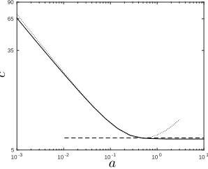
Figure 5: Comparison of wavespeeds obtained from numerical solutions to (1), (2) to pushed and pulled speeds µ= 10. Solid curve: numerical solutions; dashed curve: pulled speed; dotted curve: pushed speed, both from (24), scaled by√µ.

Figure 9 focusses onaT(µ), showing the asymptotic expressions and an attempt at a numerical criterion to identify this cross-over point (by isolating pairs (a, µ) for which the numerically obtained speed deviates from that given by (4), (5) by less than 1%). Given the insensitivity of the wavespeed at small µ with a≫ µto whether the front is pulled or pushed, the quality of the agreement for smallµis unsurprising, but that for largeµis encouraging.

7

Discussion

In this study, we have considered in detail the propagation of monotonic travelling wave solutions to a spatially-discrete diffusion equation with cubic nonlinearity on a one-dimensional integer lattice. The focus of this work was on characterising, for the first time, the transition between so-called ‘pulled’ (where the propagation speed is characterised by the leading-edge behaviour) and ‘pushed’ (the entire nonlinear wave profile determines the wavespeed) fronts, under variation of the coupling strength µ and of the detuning parameter a that appears in the nonlinear term. While results characterising the transition between pushed and pulled fronts in the continuum version of the equation studied herein are well established (seee.g.Hadeler and Rothe [20], Stokes [21] and Rothe [27]), and the linearly-selected speed of travelling waves in discrete systems is straightforward to obtain, we are not aware of previous detailed results for pushed waves in discrete equations.

0 0.05 0.1 0.15 0.2 0.25 0.3 0.1

0.12 0.14 0.16 0.18 0.2 0.22 0.24 0.26 0.28 0.3

a

c

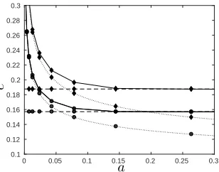
Figure 6: Comparison of wavespeeds obtained from numerical solutions to (1), (2) (solid lines) against asymptotic pushed speeds (74) (dotted lines) and exact pulled speed (4), (5) (dashed lines). The curves marked with circles are forµ= 10−4_{, and those with diamonds forµ= 6×10−}4_.

0.04 0.06 0.08 0.1 0.12 0.14 0.16 0.18 0.2 0.14

0.145 0.15 0.155 0.16 0.165 0.17 0.175 0.18 0.185 0.19

a

c

Figure 7: Comparison of the asymptotic speeds for pushed (94) (dotted line) and pulled (31) (dashed line) waves, with numerical simulation results (solid line) for an intermediate range ofaandµ= 10−4_. The figure also illustrates the tangency of the pulled and pushed curves at the transition point.

(a)cmin(a, µ) =c∗_{(µ) fora > aT(µ). c}∗_{(µ)>0 is given exactly by (see (4), (5))}

λ∗c∗= 2µ(cosh(λ∗)−1) + 1, c∗= 2µsinh(λ∗), (96) or, equivalently, by the transcendental equation

c∗ln c∗+

p

c∗2_{+ 4µ}2

2µ

!

=pc∗2_{+ 4µ}2_{−2µ+ 1. (97)}

(b)cmin(a, µ) =c†_{(a, µ)∼} 2 π

pµ

a, asa→0

+ _{at fixedµ, this following from (106).}

Figure 8 compares these results to the numerical ones.

The asymptotic results in terms of µ can be summarised as follows. Two distinguished limits arise whenµ≪1, in which caseaT(µ)∼1/ln(1/µ).

(I)a=O(µ) (pushed)

c†(a, µ)∼



    

    

√

(4µ/a)−1 2

1 tan−1“√_(4µ/a)

−1”, 0< a <4µ;

1/2, a= 4µ;

√

1₋(4µ/a) 2

1 tanh−1“√₁

−(4µ/a)”, a >4µ.

(98)

10-3 10-2 10-1 100 101

100

101

a

c

Figure 8: Comparison of wavespeeds obtained from numerical solutions (solid lines) with the pulled speed from (4), (5) (dashed lines) and the smallabehaviour of the pushed speedc† _∼2p

(µ/a)/π

(dotted lines) given by (71), forµ= 0.43 (bottom), 1.6,3 (top).

10-1 100

10-4

10-3

10-2

10-1

100

101

a

µ

Pulled Pushed

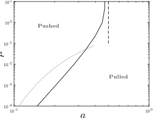
Figure 9: Contours in a, µ-space indicating the transition between pushed and pulled wavefronts. The solid line demarks the set of parameter values for which the pulled speed (4), (5) provides a good estimate of the speed observed in numerical simulations: for parameter values lying to the right of this curve, (4), (5) deviates from the numerical speed observed in numerical simulations by less than 1%. Also shown is the transition contour given by (91) (valid in the weak-coupling limit

µ≪1; dotted line) and the transition valueaT = 1/2 (pertaining to the PDE (7); dashed line).

(II)a=O(1/ln (1/µ)) (transition)

c†_{(a, µ)∼} 1

ln(1/µ)+

aln(1/µ)−lna

ln2(1/µ) , 0< aln(1/µ)<1; (99)

c∗_(µ)∼ 1

ln(1/µ)+

ln ln(1/µ) + 1

ln2(1/µ) , aln(1/µ)>1; (100)

the latter expression for c∗ _{of course (because pulled speeds are independent of a) also holds for}

a>O(1).

Figure 7 is devoted to a comparison in this regime.

Forµ≫1 we instead have the following, withaT(µ)∼1/2. (A)a=O(1/µ) (pushed)

c†(a, µ)∼cˆmin(aµ)/a (101)

where ˆcminis determined as in Appendix A via (104).

(B)a=O(1) (withcscaled as in (26)); see Figure 5 for a comparison.

c†(a, µ)∼√2a+ 1/√2a√µ, 0< a <1/2 (pushed); (102)

Figures 2 and 5 illustrate the applicability of these results.

The correction terms to the asymptotic results (b), (I), (A) and (B) are algebraic in the relevant small parameter, while those in (II) are only logarithmically small; this distinction is clearly reflected in the comparisons above with the numerical results.

We note that in the weak-coupling limit analytical expressions are thus available for the wavespeed in both pulled and pushed regimes and, unlike those for the continuum limit, the latter can relatively easily be generalised to other forms of nonlinearity. It is important to stress that the pulled speed is available through the transcendental expression in (a) for arbitraryµ and is independent of a, depending only on the problem linearised aboutu= 0; by contrast, the pushed speed is much more challenging to obtain and the transition point aT(µ) is extremely difficult to get at, even numeri-cally (particularly given that the transition between pulled and pushed occurs rather smoothly, as described in§4).

A number of conjectures warranting rigorous investigation, such as thataT(µ) is an increasing function of µ (contrast Appendix C) arise naturally from this work. Similarly, obvious potential extensions come to mind, the higher-dimensional generalisation being the subject of current study.

8

Acknowledgements

This work was initiated with funding from Biotechnology and Biological Sciences Research Council and Engineering and Physical Sciences Research Council (BB/D008522/1), which we gratefully acknowledge.

Appendices

A

The limit

a

_→

0

in (2)

The system (1), (2) contains two parameters, µ and a; the bulk of this paper focusses on the dependence on the former, while here we briefly address the latter. The limit a→+∞is a regular one in which the ‘u/a’ term inf(u;a) is simply disregarded at leading order and the front is a pulled one (that the front is pulled whena→+∞for anyµis a conjecture based on the results above; a stronger conjecture also suggested by our results is that aT(µ) is an increasing function ofµ with

aT(∞) = 1/2, andaT(µ)∼1/ln(1/µ) asµ→0+). We are therefore concerned here with the limit

a→0+_{when pushed fronts are to be expected.}

If we set µ= ˆµ/a,c= ˆc/aand take the limita→0, (26) becomes

ˆ

µ(U(z+ 1)−2U(z) +U(z−1)) + ˆcdU(z)

dz +U

2_{(z)(1−U(z)) = 0 (104)}

and it is cleara priori that the wave must then be pushed (the linearisation off(u) being trivial); moreover, absorbingaby the above rescaling implies

cmin(a, µ)∼ˆcmin(aµ)/a asa→0+, µ=O(1) (105) and the preceding analyses of pushed fronts imply with minor modifications that

ˆ

cmin(ˆµ)∼pµ/ˆ 2 as ˆµ→+∞,cˆmin(ˆµ)∼2pµ/πˆ as ˆµ→0+ (106) (cf.(22) and (74) asα→+∞). It is noteworthy in (106) that ˆcminscales with ˆµin the same fashion in both limits.

B

A linear differential-difference equation

The differential-difference equation

d

dξv(ξ+ 1) +σv(ξ) = 0 (107)

plays a central role in §5.4 and warrants brief separate discussion, not least because it constitutes a rare instance in which the appropriate treatment of a linearised problem in such a wavespeed-selection analysis isnot simply the Liouville-Green (or JWKB) approximation. The notation in this appendix differs from elsewhere.

Introducing the Laplace transform

ˆ

v(ρ) =

Z ∞

0

v(ξ)e−ρξdξ, v(ξ) = 1

2πi

Z i∞

−i∞

ˆ

v(ρ)eρξdρ, (108)

(the poles of ˆv(ρ) haveR_{(ρ)<0) gives}

(ρeρ+σ)ˆv(ρ) =v(1) +ρeρ

Z 1

0

v(ξ)e−ρξ_{dξ. (109)}

The poles of ˆvthus occur atρ=−λwith

λe−λ_{=σ (110)}

(cf.(63)), so forσ <1/e there are two (real) roots for λthat we denote here byλ₋ and λ+, with

0< λ₋< λ+, and it is easy to show that the complex roots all have real part larger thanλ+.

Equation (107) requires initial data for 06ξ61 and for our purposes in§5 it suffices to consider the case

v(ξ) = eνξ for 06ξ61 (111)

for constantν, and it then follows from (109) that

(ρeρ+σ)ˆv(ρ) = ρe ρ_−νeν

ρ−ν . (112)

Ifν=−λ, withλsatisfying (110), we have ˆ

v(ρ) = 1/(ρ+λ), v(ξ) = e−λξ_{, (113)}

as is clear beforehand. More significantly for our purposes, the far-field behaviour

v(ξ)∼ λ−+νe

λ−+ν

(1−λ−)(λ−+ν)

e−λ−ξ, asξ→ ∞ (114)

follows from (112) as a residue contribution; suppressing such a slowly decaying term is a central ingredient in the selection mechanism for a pushed front in§5.4.

C

Pulled and pushed waves in a discrete diffusion equation

with nonlinear coupling

In this appendix, we show that travelling wave speeds for (1), with nonlinearity given by (2), may be constructed explicitly in both the pushed and pulled regimes in the case for which constant coupling strength is replaced by the nonlinear function

µ= µu

2 j

uj+1uj₋1

in which µ is constant. The nonlinearity (115) converges to the constant-coupling case in the continuum (slowly varying) limit and is otherwise mathematically convenient, as we shall highlight below.

Travelling wavesU(z), propagating at speedc obey

µU2_(z)

U(z+ 1)U(z−1)(U(z+ 1)−2U(z) +U(z−1)) +c dU(z)

dz +f(U(z);a) = 0. (116)

C.1

Stable–unstable connections

I Pulled waves Because

U(z)∼e−λz _{z→+∞ (117)}

hasµ∼µin (115), the pulled wavespeedc∗_{(µ) is again given by (4), (5).}

II Pushed waves Wave propagation speeds determined by the whole nonlinear wavefront may be obtained by the ansatz (which motivated (115) in the first place)

U(z) = 1

V(z), V(z) = 1 + e

λz_{. (118)}

We thereby obtain

cV(z)dV(z)

dz −µ(V(z)V(z+ 1)−2V(z+ 1)V(z−1) +V(z)V(z−1))−(V(z)−1)

V(z) +1

a

= 0,

(119) and hence

c†_λ†_{= 2µ cosh(λ}†₎₋₁

+ 1, c†_λ† _{= 1 +} 1

2a, (120)

with a pushed front occuring when λ† _{> λ}∗_{; λ}†_{(a, µ) and c}†_{(a, µ) can be determined explicitly in}

the form

λ†_{= ln}

1 +1 +

√

1 + 8aµ

4aµ

, c†_{= (1 + 1/2a)/λ}†_{, (121)}

and the transition relationshipsλ† _=λ∗_,c† _=c∗ _{imply thata}

T(µ) is given by

2aT+ 1 =

p

1 + 8aTµln

1 + 1 +

√

1 + 8aTµ 4aTµ

. (122)

Equation (116) is evidently not of the class discussed in Appendix D; moreover, setting

U(z)∼e−λ∗_z

W(z) (123)

in (116) withc=c∗ _{andW(z) slowly varying yields the dominant balance}

2(cosh(λ∗₎₋₁₎

W

_dW

dz

2

−Wd

2_W

dz2

!

+ cosh(λ∗₎d2W

dz2 = 0, (124)

so the far-field behaviour differs from (37), and the behaviour outlined in Appendix D might not be expected to pertain. Nevertheless, it is easy to see that∂c†_(a

T, µ)/∂a= 0 also holds in this case. Equation (121) implies

c† ∼_2aln(11_/2aµ) as a→0+, c† ∼p2aµasa→+∞, (125)

the former being consistent with the scaling argument embodied by (105) and the latter correspond-ing to the continuum limit. More importantly,

c† _{∼(1 + 1/2a)/ln(1/2aµ) asµ→0}+_{, c†}

100 ₁₀1

10-6

10-5

10-4

10-3

10-2

10-1

100

101

102

a

µ

Figure 10: The transition contouraT(µ) (solid line) as given by (122), separating regions of param-eter space in which pulled and pushed fronts arise in (1) with coupling strength and nonlinearity given by (115) and (2), respectively. Also shown are the results corresponding to the strong (dashed line) and weak-coupling (dotted line) limits (127).

and it follows that

aT ∼ln(1/µ)/2 asµ→0+, aT ∼1/2 asµ→+∞; (127) the latter is as expected from the continuum limit, but the former implies aT → +∞ as µ→0+,

i.e.the opposite behaviour from that in§5.4. Thus the analysis of (119) is counterproductive in terms of gaining insight into (26) – it does, however, reinforce the point that intuition into whether pushed or pulled behaviour is to be expected is hard to come by in the weakly-coupled case. Figure 10 shows the curve (122) separating pushed and pulled waves, together with the weak- and strong-coupling limits (127). The offset of the latter for µ ≪ 1 illustrates further the implications of logarithmic terms in the associated asymptotic expansions (here through closed-form expressions, in contrast to

§5.4).

C.2

Stable–stable connections

For completeness, we exploit the analytic tractability of (115) to address this case also. For a connection between the stable states U = 1,−a(stable for a >0), representing the propagation of the stateU =−aoverrunningU = 1 (andvice versa, denoted ˜U) we set

U(z) = 1−1 +_V(za₎, U˜(z) =−a+1 +a

V(z), (128)

where V(z) is defined in (118). In each case, the wavespeed and decay rate may be obtained as in

§C.1. The resulting wavespeeds are

c±=±₂1_λ

a−1_a

, (129)

wherec+_{corresponds to the waveU(z) andc−to ˜U, and the decay rateλ(µ, a) is given in each case} by

λ(µ, a) = cosh−1

1 + (a+ 1) 2

4aµ

; (130)

indeed the ostensibly distinct solution ans¨atze (128) in fact represent the same propagating front, moving in opposite directions.

D

The generic pushed/pulled transition

Here we revisit briefly the analysis of§4 in a much more general setting. We consider the travelling-wave problem

P

d dz

U+cdU

for a pseudo-differential operator with symbolP, whereby

P

_d

dz

e−λz_=P(−λ)e−λz ₍₁₃₂₎

and the analysis henceforth will for the most part depend on P only in the form of the function

P(−λ); for the discrete problem (1),P(−λ) is

P(−λ) = 2µ(cosh(λ)−1). (133)

We again let

f(u;a) =u+o(u) asu→0 (134)

and assumeP andf are such that for any givenc >0 a unique connection satisfying

U →1 asz→ −∞, U→0 asz→+∞, U(0) = 1/2 (135) exists. Asz→+∞we will in general have (39), whereλis a root of

P(−λ)−λc+ 1 = 0 (136)

with smallest real part. The repeated root case hasc∗ _andλ∗ _{determined by}

P(−λ∗_)−λ∗_c∗_{+ 1 = 0, −P}′_(−λ∗_)−c∗_{= 0, (137)}

in which caseU satisfies (37). The transition valuea=aT is given byA(aT) = 0 with, generically,

B(aT)>0, and we again take the dependence off uponato be such that a pulled front arises for

a < aT and a pushed one fora > aT.

In the Liouville-Green approach (14), we have

∂φ

∂t +P

−∂φ_∂x

+ 1 = 0, F −ηdF

dη +P

−d_dF_η

+ 1 = 0; (138)

on the envelope solution to the second of these (i.e. the Clairaut equation)

0 =−P′

−d_dF_η

−η (139)

holds, so by (137) it follows that F = 0 on η =c∗_{, dF/dη = λ}∗_{, as is to be anticipated.}

Corre-spondingly, the expansion-fan solution of the first of (138), parameterised byq=∂φ/∂x(which is constant on rays) is

x=−P′(−q)t, φ=−(qP′(−q) +P(−q) + 1)t, (140) and determining whereφ= 0 gives a further derivation of the same result.

Again settinga=aT+δ,λ∼λ∗−δΛ and adopting the expansion (43) implies

P

−_dd_x

U0+c∗dU0

dz +f(U0;aT) = 0, P

−_dd_x

U1+c∗dU1

dz + ∂f

∂u(U0;aT)U1=−

∂f

∂a(U0;aT),

(141) from which we recover (44). Equations (136), (137) imply

1 2P

′′_(−λ∗_)Λ2_=λ∗_{C; (142)}

a pushed front (wherebyδ <0) hasC >0, Λ>0 (and henceP′′_(−λ∗_{)>0) so by (40)}

U† ∼A†+(aT) +δ

A†′+(aT) + ΛA†+(aT)z

e−λ∗z asδ→0−, z→+∞ (143) and consistency with (44) demands

and hence

C= 1

2λ∗P′′(−λ∗) (A′(aT)/B(aT))

2

. (145)

Finally,

P

− d

dx

U2+c∗dU2

dz + ∂f

∂u(U0;aT)U2=−

∂2_f

∂a2(U0;aT)−2

∂2_f

∂a∂u(U0;aT)u1−

∂2_f

∂u2(U0;aT)u

2 1−C

dU0 dz ,

(146) the last term in which dominates the right-hand side asz→+∞and implies

U2∼λ

∗_B(aT)C

2P′′_(−λ∗₎z

2_e−λ∗_z

asz→+∞; (147)

matching this to the corresponding term from (40) again implies (142), representing a useful consis-tency check.

Salient features arising from the above (providing one of the motivations for this more general analysis) include the following.

1. The wavespeed c∗ _{in the pulled front case, given by (137), is independent ofa; this is}

self-evident from the nature (134) of the linearisation, but is important to stress. Correspondingly, in the current limit, that the pre-exponential in (37) has no term quadratic in z has the consequence that (147) implies C≡0 for a pulled front.

2. In the pulled-front case the wavespeed is accordingly knowna priori from (137); solving (131) for this wavespeed determines A(a) and B(a) in (37) and hence, through (144), (145), fully determines the pushed-front behaviour (wherein c has in general instead to be treated as an eigenvalue, being found as part of the solution) local to the transition.

3. The resultc†_−c∗_{=O((aT −a)}2_{) asa}

→a−T seems to be generally applicable.

References

[1] Cahn JW (1960) Theory of crystal growth and interface motion in crystalline materials. Acta Metall. 8(8):554–562.

[2] Cahn JW, Chow SN, Vleck van ES (1995) Spatially discrete nonlinear diffusion equations. Rocky Mountain J Math 25:87–118.

[3] Chua LO Yang L (1988) Cellular neural networks: Applications. IEEE Trans Circuits Syst 35: 1273–1290.

[4] Chua LO Yang L (1988) Cellular neural networks: Theory. IEEE Trans Circuits Syst 35: 1257–1272.

[5] Ma S Zou X (2005) Existence, uniqueness and stability of travelling waves in a discrete reaction-diffusion monostable equation with delay. J Diff Eq 217:54–87.

[6] Owen MR (2002) Waves and propagation failure in discrete space models with nonlinear cou-pling and feedback. Phys D: Nonlin Phenomena 173(1-2):59–76.

[7] Muratov C.B. Shvartsman S.Y. (2004) Signal propagation and failure in discrete autocrine relays. Phys Rev Lett 93(11):118101(1–4).

[8] Plahte E Øyehaug L (2007) Pattern-generating travelling waves in a discrete multicellular sys-tem with lateral inhibition. Phys D: Nonlin Phenomena 226(2):117–128.

[10] Cook HE, De Fontaine D, Hilliard JE (1969) A model for diffusion on cubic lattices and its application to the early stages of ordering. Acta Metall 17:765–773.

[11] Keener JP (1987) Propagation and its failure in coupled systems of discrete excitable cells. SIAM J Appl Math 47:556–572.

[12] Elmer CE Vleck van ES (1996) Computation of travelling waves for spatially discrete bistable reaction-diffusion equations. Appl Num Math 20(1):157–170.

[13] Cahn JW, Mallet-Paret J, Van Vleck ES (1998) Travelling wave solutions for systems of ODEs on a two-dimensional spatial lattice. SIAM J Appl Math 59(2):455–493.

[14] Chow SN, Mallet-Paret J, Shen W (1998) Traveling waves in lattice dynamical systems. J Diff Eq 149:248–291.

[15] F´ath G (1998) Propagation failure of travelling waves in a discrete bistable medium. Physica D: Nonlin Phenom 116(1-2):176–190.

[16] King JR Chapman SJ (2001) Asymptotics beyond all orders and stokes lines in nonlinear differential-difference equations. Eur J Appl Math 12:433–463.

[17] Zinner B, Harris G, Hudson W (1993) Travelling wavefronts for the discrete Fisher’s equation. J Diff Eqs 105:46–62.

[18] Guo J.S. Morita Y. (2005) Entire solutions of reaction-diffusion equations and an application to discrete diffusive equations. Discrete Contin Dyn Syst 12:193–212.

[19] Hakberg B (2013) A discrete KPP-theory for fisher’s equation. Math Comp 82:781–802.

[20] Hadeler KP Rothe F (1975) Travelling fronts in nonlinear diffusion equations. J Math Biol 2 (3):251–263.

[21] Stokes AN (1976) On two types of moving front in quasilinear diffusion. Math Biosci 31(3-4): 307–315.

[22] Lucia M, Muratov CB, Novaga M (2004) Linear vs. nonlinear selection for the propagation speed of the solutions of scalar reaction-diffusion equations invading an unstable equilibrium. Comm Pure Appl Math 57:616–636.

[23] Fisher RA (1937) The wave of advance of advantageous genes. Ann Hum Gen 7:355–369.

[24] Kolmogorov AN, Petrovskii IG, Piskunov NS (1937) A study of the equation of diffusion with increase in the quantity of matter, and its application to a biological problem. Bul Moskovskogo Gos Univ 1:1–26.

[25] Saarloos van W (2003) Front propagation into unstable states. Physics Reports 386:29–222.

[26] Cuesta CM King JR (2010) Front propagation in a heterogeneous Fisher equation: The homo-geneous case is non-generic. Q J Mech Appl Math 63:521–571.