Ground Ozone Level Prediction Using Machine Learning

ISSN Online: 1945-3124 ISSN Print: 1945-3116

DOI: 10.4236/jsea.2019.1210026 Oct. 29, 2019 423 Journal of Software Engineering and Applications

Ground Ozone Level Prediction Using Machine

Learning

Zhiying Meng

Beijing National Day School, Beijing, China

Abstract

Because of the increasing attention on environmental issues, especially air pollution, predicting whether a day is polluted or not is necessary to people’s health. In order to solve this problem, this research is classifying ground ozone level based on big data and machine learning models, where polluted ozone day has class 1 and non-ozone day has class 0. The dataset used in this research was derived from the UCI Website, containing various environmen-tal factors in Houston, Galveston and Brazoria area that could possibly affect the occurrence of ozone pollution [1]. This dataset is first filled up for further process, next standardized to ensure every feature has the same weight, and then split into training set and testing set. After this, five different machine learning models are used in the prediction of ground ozone level and their fi-nal accuracy scores are compared. In conclusion, among Logistic Regression, Decision Tree, Random Forest, AdaBoost, and Support Vector Machine (SVM), the last one has the highest test score of 0.949. This research utilizes relatively simple methods of forecasting and calculates the first accuracy scores in predicting ground ozone level; it can thus be a reference for envi-ronmentalists. Moreover, the direct comparison among five different models provides machine learning field an insight to determine the most accurate model. In the future, Neural Network can also be utilized to predict air pollu-tion, and its test scores can be compared with the previous five methods to conclude the accuracy of Neuron Network.

Keywords

Ground Ozone Pollution, Machine Learning, Classification, Logistic Regression, Decision Tree, Random Forest, AdaBoost, Support Vector Machine

1. Introduction

Ground ozone pollution has been a serious air quality problem over the years How to cite this paper: Meng, Z.Y. (2019)

Ground Ozone Level Prediction Using Ma-chine Learning. Journal of Software Engi-neering and Applications, 12, 423-431. https://doi.org/10.4236/jsea.2019.1210026

Received: September 11, 2019 Accepted: October 26, 2019 Published: October 29, 2019

Copyright © 2019 by author(s) and Scientific Research Publishing Inc. This work is licensed under the Creative Commons Attribution-NonCommercial International License (CC BY-NC 4.0). http://creativecommons.org/licenses/by-nc/4.0/

DOI: 10.4236/jsea.2019.1210026 424 Journal of Software Engineering and Applications and can be extremely harmful to people’s health if no advanced forecasts are provided. However, the occurrence of an ozone polluted day depends on a lot of sophisticated chemical, physical, and geological factors, so it is too complicated and indirect to use simple math formula to calculate the ozone level. Fortunate-ly, a group of scientists measured several environmental factors in Houston, Galveston and Brazoria area that might influence ground ozone pollution, which is the dataset used in this research. This group also utilized the same dataset to build models that can successfully predict the ground ozone level. Their paper,

Forecasting Skewed Biased Stochastic Ozone Days: analysis, solutions and

beyond, published in April 2007, researched about data mining techniques based on the collected dataset and had made huge improvements on the Huston ground ozone pollution forecasting system. On the other hand, in this research, five different machine learning models are trained to make binary predictions of ground ozone level (ozone day: 1, non-ozone day: 0).

Besides providing precise forecasting system for the citizens, this research also contributes to the field of machine learning. With the employment of five dif-ferent models, the accuracy scores can be compared and the conclusion that which method is the most accurate can be derived relatively simple and clear. During the construction of each method, variables are changed five times to maximize each model’s test scores. These scores are eventually used to compare the accuracy of each method and select the most precise one as the best predic-tion method.

2. Data Description and Preprocessing

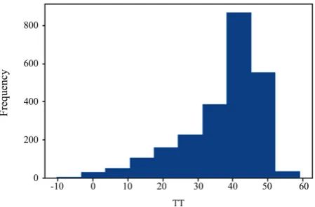
This dataset is downloaded from the UCI website, called Ozone Level Detection Data Set. It includes 2536 instances with 73 attributes, containing only 1 date data and 72 numeric data. Features like T (temperature), WSR (wind speed re-sultant), RH (relative humidity), U (u wind: east-west direction wind), V (v wind: north-south direction wind), HT (geopotential height), KI (k index: thun-derstorm potential), TT (t totals: assess storm strength), SLP (sea level pressure), SLP_ (SLP changes from yesterday), Prep (precipitation) are measured each day for 24 hours constantly from 1998.1.1 to 2004.12.31, although a great number of missing values are present. The maximum number of missing values of one fea-ture is 299 in WSR0, and most data is continuously missing on the first 53 attributes from 7/1/2002 to 1/20/2003. The final prediction is binary, 0 means that day is non-ozone day and 1 means that day is polluted. In this dataset, about 2300 instances are classified as non-ozone days and 200 as ozone-days.

DOI: 10.4236/jsea.2019.1210026 425 Journal of Software Engineering and Applications next year’s data. The following steps are all based on this filled dataset.

For the purpose of checking the accuracy of this final classification model, it is divided into two groups with 70% of the data as the training set and 30% as the testing set.

Figure 1. The average wind speed in one day has maximum frequency around 2 and lower frequency as the speed gets lower or higher than 2.

Figure 2. Almost 95% of precipitation values are 0, only in a few days, there are values from 1 to 10.

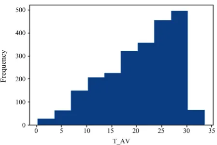
DOI: 10.4236/jsea.2019.1210026 426 Journal of Software Engineering and Applications Figure 4. The average temperature in one day has

frequencies steadily increasing from 0 to 30 degrees, and suddenly fell down between 30 and 35.

On the other hand, Z scale is used to standardize the dataset so that all the attributes will have the same weight. The data after compression x’ = (x − u)/xrms, where u is the mean value and xrms is its root-mean-square value calculated with the formula below.

2 2 2

1 2 n

rms x x x

x

n

+ + +

= 

3. Analysis with Different Machine Learning Models

3.1. Principal Component Analysis (PCA) and Logistic Regression

Logistic Regression [2] is a statistical model using a logistic function to predict binary outcomes. Since this dataset contains too many attributes, feature attrac-tion is needed before building the actual machine learning model. Principal Component Analysis (PCA) [3] is a statistical procedure that is used to convert a set of possible related variables into a set of linearly uncorrelated variables called principal components, which means to reduce the dimensions of this dataset and select some principal features.

As stated in the introduction part, one of the goals of this research is to de-termine the number of principle features chosen, so different constants from 30 to 70 are tried in building the logistic regression models and calculating the ac-curacy scores respectively. After repeating the same steps of logistic regression for 10 times, the mean values of scores of the same constant can be calculated and compared with others.

DOI: 10.4236/jsea.2019.1210026 427 Journal of Software Engineering and Applications Eventually, we can see that when choosing 72 numbers of principal compo-nents, which has the exact effect of not using PCA to extract features, the ma-chine learning model is the most accurate one. In conclusion, this dataset doesn’t need feature reduction to produce a better model, so the final logistic re-gression model is influenced by all 72 attributes of the original dataset, with the highest train and test scores of 0.859 and 0.800 (see from Figure 5).

3.2. AdaBoost

AdaBoost [4], the abbreviation of Adaptive Boosting, is a lifting algorithm com-bining multiple weak classifiers to form one strong classifier. This model adapts this dataset by increasing the weights of wrongly classified instances and lower-ing the correctly classified instances’ weights, then uslower-ing the updated parameters to train the next week classifier. This iteration continues until the designated er-ror rate or the maximum iteration times is reached. When combining all week classifiers together, those with higher accuracy rate are added with higher weights while the less accurate ones have lower weights.

The parameter in this model is n_estimators, which is the numbers of week classifiers that will be added together to form the final learning model. It is va-ried from 300 to 700 to find the highest accuracy testing score possible without overfitting. When the n_estimators is set to 400, the train and test scores are the highest: 0.970 and 0.938 (see from Figure 6).

3.3. Decision Tree

The second method used to predict the ozone level is Decision Tree [5], which is a symbol of the mapping relation between the objects’ features and their values. Each node in the tree stands for one object, each split branch stands for some possible attributes of this object, and the path from each leaf node to the root node is the value of the leaf node. The criterion for this decision tree is entropy, which means the uncertainty of the random variables. The smaller the entropy is, the less uncertainty the data has, so we want to lower the entropy as much as possible.

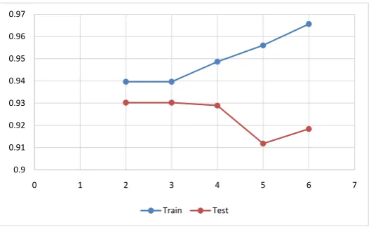
Max depth, the length of the longest path from the tree root to a leaf, is one variable in this machine learning model and is changed from 2 to 6. As this graph shows, the best train and test scores are about 0.940 and 0.930 respectively when max depth is 3 (see from Figure 7).

3.4. Random Forest

Random Forest [6] is a general technique of random decision forest, which con-structs multiple decision trees at a training time and output the class as the mode or mean of the classification of individual trees. This model is using a simple bagging thinking, and is similar to the principle of AdaBoost.

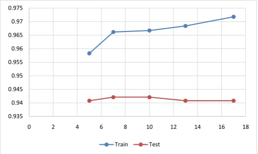
DOI: 10.4236/jsea.2019.1210026 428 Journal of Software Engineering and Applications value of max depth is also settled because the decision tree model shows the best accuracy when it is set at 3. Another variable, max features, is the size of random feature subsets to consider when splitting a node, and is set as five different val-ues from 5 to 17. The Random Forest model eventually reach the maximum scores at the value of 7 (train: 0.966; test: 0.942) (see from Figure 8).

Figure 5. Logistic Regression accuracy scores with different numbers of Principle Components.

Figure 6. AdaBoost accuracy scores with different n_estimators.

Figure 7. Decision Tree accuracy scores with different max_depth. 0.78

0.79 0.8 0.81 0.82 0.83 0.84 0.85 0.86 0.87

0 10 20 30 40 50 60 70 80

Train Test

0.92 0.93 0.94 0.95 0.96 0.97 0.98 0.99

0 100 200 300 400 500 600 700 800

Train Test

0.9 0.91 0.92 0.93 0.94 0.95 0.96 0.97

0 1 2 3 4 5 6 7

DOI: 10.4236/jsea.2019.1210026 429 Journal of Software Engineering and Applications Figure 8. Random Forest accuracy scores with different max_features.

3.5. Support Vector Machine (SVM)

SVM [7] is a machine learning model using kernel method (non-linear regres-sion) to make binary predictions. In linear SVM, data is first transferred to an eigenspace by non-linear mapping, then a linear machine learning method is used to classify data. Linear SVM’s decision rule can be shown using the inner product of train and test sets. Kernel method, on the other hand, is able to di-rectly calculate the inner product inside eigenspace, thus can handle non-linear division problems. The first variable kernel is set as “rdf”, meaning to use kernel method instead of linear classification; the second variable gamma is set as “au-to”, standing for automated choosing kernel constants.

By adjusting different values of error tolerance C, the third variable, from 7 to 20, the highest train score 0.984 and test score 0.949 are reached when C equals to 13 (see from Figure 9).

4. Conclusions

Ground ozone pollution is considered as a very serious environmental problem due to its strong influence on people’s health; therefore, a more accurate fore-casting system is certainly a necessity.

Based on the dataset provided by the UCI website, this research is able to cor-rectly predict the air pollution in Bostn area according to various attributes of the location and its weather. This research used five different methods to classify the ground ozone level by indicating whether the day is an ozone day (class = 1) or not (class = 0). However, some limitations of this prediction are that there are a lot of original missing values and that the instances are too small for more pre-cise model training. After solving these problems, machine learning models are trained by changing variables in order to create the best models.

Considering about the large number of attributes, Principal Component Analysis (PCA) is applied first to maximize the accuracy which is calculated us-ing logistic regression. Since the score is the highest when the total 72 features are considered, PCA is proven to be unnecessary. The following methods are AdaBoost, decision tree, random forest, and Support Vector Machine (SVM).

0.935 0.94 0.945 0.95 0.955 0.96 0.965 0.97 0.975

0 2 4 6 8 10 12 14 16 18

DOI: 10.4236/jsea.2019.1210026 430 Journal of Software Engineering and Applications Figure 9. Support Vector Machine accuracy scores with different

error tolerance (C).

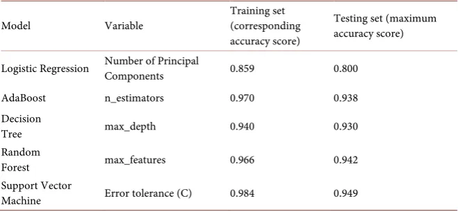
Table 1. Accuracy scores comparison for five machine learning models.

Model Variable Training set (corresponding accuracy score)

Testing set (maximum accuracy score)

Logistic Regression Number of Principal _Components 0.859 0.800

AdaBoost n_estimators 0.970 0.938

Decision

Tree max_depth 0.940 0.930

Random

Forest max_features 0.966 0.942

Support Vector

Machine Error tolerance (C) 0.984 0.949

Eventually their train and test scores are compared and this research reached a conclusion that using SVM to predict binary outcomes is the most accurate me-thod, which has the highest test score of 0.949 (see from Table 1).

In the future, I will probably try classifying this data using Neural Network or Deep Learning techniques, and then compare their accuracy scores with the preceding five methods.

Acknowledgements

This has been an amazing experience for me. I gained a lot of experience of pro-gramming and got more opportunities because of things I learnt from this class.

Thanks to Professor Pradeep Ravikumar who taught me machine learning and gave me really helpful advices to improve my research paper.

Thanks to CIS program which provided me with such a great platform to learn useful knowledge and publish my own paper.

Thanks to all people who provided me their help and suggestions.

Conflicts of Interest

The author declares no conflicts of interest regarding the publication of this paper. 0.94

0.945 0.95 0.955 0.96 0.965 0.97 0.975 0.98 0.985 0.99

0 5 10 15 20 25

DOI: 10.4236/jsea.2019.1210026 431 Journal of Software Engineering and Applications

References

[1] Dua, D. and Graff, C. (2019) UCI Machine Learning Repository. School of Informa-tion and Computer Science, University of California, Irvine, CA.

http://archive.ics.uci.edu/ml

[2] Jolliffe, I. (2011) Principal Component Analysis. Springer, Berlin Heidelberg.

https://doi.org/10.1007/978-3-642-04898-2_455

[3] Li, S.S. (2019) Building A Logistic Regression in Python, Step by Step. Medium, Towards Data Science, 27 Feb.

https://towardsdatascience.com/building-a-logistic-regression-in-python-step-by-st ep-becd4d56c9c8

[4] AdaBoost Classifier in Python. DataCamp Community.

https://www.datacamp.com/community/tutorials/adaboost-classifier-python

[5] Decision Tree Classification in Python. DataCamp Community.

https://www.datacamp.com/community/tutorials/decision-tree-classification-pytho n

[6] Random Forests Classifiers in Python. DataCamp Community.

https://www.datacamp.com/community/tutorials/random-forests-classifier-python

[7] Support Vector Machines in Scikit-Learn. DataCamp Community.