tion approach for the network coding resource minimization problem. It is featured with several attractive mechanisms spe-cially devised for solving the network coding resource minimiza-tion problem: 1) a multi-dimensional pheromone maintenance mechanism is put forward to address the issue of pheromone overlapping; 2) problspecific heuristic information is em-ployed to enhance the heuristic search (neighboring area search) capability; 3) a tabu-table based path construction method is devised to facilitate the construction of feasible (link-disjoint) paths from the source to each receiver; 4) a local pheromone updating rule is developed to guide ants to construct appro-priate promising paths; 5) a solution reconstruction method is presented, with the aim of avoiding prematurity and improving the global search efficiency of proposed algorithm. Due to the way it works, the ant colony optimization can well exploit the global and local information of routing related problems during the solution construction phase. The simulation results on benchmark instances demonstrate that with the five extended mechanisms integrated, our algorithm outperforms a number of existing algorithms with respect to the best solutions obtained and the computational time.
Index Terms—Ant Colony Optimization, Network Coding, Combinatorial Optimization.
I. INTRODUCTION
T
RADITIONAL routing works in such a way that data information being transmitted is stored and forwarded at intermediate nodes in communications networks. At the network layer, data streams are processed separately as fluids share pipes or vehicles share highways [1]. Unfortunately, traditional routing cannot guarantee to achieve the maximum multicast throughput, determined by the Max-Flow Min-Cut theorem [2]. Hence, in 2000, Ahlswede et al. proposed net-work coding [3], an emerging communication paradigm that always enables the theoretical maximum data rate. Network coding has revolutionized the way of information processing and transmission in communications network. It is a great breakthrough in the field of information theory, computer science and telecommunications.The network coding resource minimization (NCRM) prob-lem is a resource optimization probprob-lem emerged in the field of
Zhaoyuan Wang, Huanlai Xing (Corresponding author, e-mail: [email protected]), Tianrui Li and Yan Yang are with School of Information Science and Technology, Southwest Jiaotong University, Chengdu 611756, China.
Rong Qu is with School of Computer Science, the University of Notting-ham, NottingNotting-ham, NG8 1BB, UK.
Yi Pan is with the Department of Computer Science, Georgia State University, Atlanta, GA 30303, USA.
Manuscript received October 20, 2014
theoretical maximum throughput of multicast, it was assumed that coding operations have to be performed at all coding-possible nodes [4]–[7]. This means all nodes which have the potential to perform coding would perform coding by default. However, as pointed out in [8]–[10], only a subset of possible nodes suffices to realize network coding-based multicast (NCM) with an expected data rate. As network coding involves complicated mathematical operations (e.g., fi-nite field computation), performing coding (and decoding) op-erations will consume significant computational and buffering resources in the corresponding nodes [11]. The less the coding operations, the less computational and buffering costs. When considering practical deployment, it is no doubt that carriers expect to make full of the benefits the NCM brings while paying minimal computational and buffering costs incurred. Therefore, it is worthwhile to study the problem of minimizing coding operations within NCM. Nowadays, Evolutionary Al-gorithms (EAs) are the mainstream solutions for NCRM in the field of computational intelligence (see Subsection III-B for details). However, the existing EAs for the NCRM problem are not good at integrating local information of the search space or domain-knowledge of the problem, which could seriously deteriorate their optimization performance.
In this paper, a modified ACO is developed for tackling the NCRM problem. Based on the framework of the basic ACO, the proposed algorithm is devised with several attractive features specially for enhancing the optimization performance. These include a multi-dimensional pheromone maintenance mechanism, the use of problem-specific heuristic information, a tabu-table based path construction method, a pheromone local updating rule, and a solution reconstruction method.
• Multi-dimensional pheromone maintenance mecha-nism. In the basic ACO, a single pheromone table is maintained. However, this always leads to a seriously de-teriorated performance when solving the NCRM problem. Hence, we develop the above pheromone maintenance mechanism to effectively solve the pheromone overlap-ping problem.
• Problem-specific heuristic information. Due to the nature of the NCRM problem, there is no clear local heuristic information immediately available for ACO to solve the NCRM problem. Hence, we devise a heuristic information scheme to provide necessary guidance to an efficient search.
• A tabu-table based path construction method. In the
NCRM problem, a set of paths is expected to be built from the source to each receiver, which is extremely difficult. To deal with this issue, we propose a tabu-table based path construction method to handle this constraint and support better collaborative performance of ants.
• A pheromone local updating rule.As constructing link-disjoint paths are quite difficult, the above path construc-tion method may not be able to produce feasible soluconstruc-tions in some complicated circumstances. Hence, a pheromone local updating rule is introduced as a complement to the path construction method above. Inappropriate path selection is punished while promising path choices are rewarded to increase the probability of generating link-disjoint paths.
• A solution reconstruction method. In order to avoid
the search being stuck in local optima and diversify the solutions, we propose a solution reconstruction method to enhance local exploitation and alleviate the premature convergence.
The rest of the paper is organized as follows. Section II introduces the basic ACO algorithm framework and the graph decomposed method for the NCRM problem. Section III describes the problem formulation and related works. Details of the proposed algorithm is introduced in Section IV. Simulation results are analyzed in Section V. Conclusions are presented in Section VI.
II. BASIC CONCEPTS
In this section, we briefly review the framework of the basic ACO and the graph decomposition method for the NCRM problem.
A. ACO
ACO was originally created to address the Traveling Sales-man Problem (TSP). Hence, this subsection describes the procedure of the basic ACO for TSP as an example [14], [20].
Given a number of cities, the objective of TSP is to find a minimal travel distance while traversing each city once. Assume there arencities fully connected by edge setE. The search procedure is shown below.
1) Initialization. Randomly selectm cities and place each city with an ant. Set initial pheromone value on each edge to a very small positive variable τ0.
2) Path construction. Ant k (k=1, 2, ..., m) (in city i) decides the next cityjto visit, according to the transition probability given in formula (1).
p(i, j) =
[τ(i,j)]α[η(i,j)]β
P
u∈Ψi
[τ(i,u)]α[η(i,u)]β, j∈Ψi
0,otherwise
(1)
Let τ(i, j) represent the pheromone on edge(i, j) and η(i, j) = 1/dijbe the heuristic information on edge(i, j) reflecting local information, where dij is the distance from cityi toj. LetΨi denote an edge set that records all edges an ant could visit. Let α, β denote weight factors, which measure the relative importance between the pheromone and the heuristic information.
3) Implement local search to optimize the solution found by antk(optional) [21]. If all ants have completed Step 2, go to Step 4. Otherwise, go to Step 2.
4) Update the pheromone level by formula (2)
τ(i, j) = (1−ρ)τ(i, j) +ρ∆τ(i, j) (2)
where the parameter ρ∈(0,1) represents the evapora-tion coefficient. The term∆τ(i, j)is associated with the performance of each ant.
5) If the termination condition is met, stop the procedure and output the best solution obtained.
B. The graph decomposition method
A communication network can be modeled as a directed graph G(V, E) where V andE denote the set of nodes and links, respectively. Assume each link e ∈ E is with a unit capacity. We refer to each non-receiver node with multiple incoming links as a merging nodewhich can perform coding operation if necessary. However, it is difficult to determine whether coding is needed at a merging node and how coding is performed when needed. In order to clearly show all possibilities when an information flow joins a merging node, the graph decomposition method was proposed to decompose a merging node into a set of auxiliary nodes connected with auxiliary links [9], [10]. The following describes the graph decomposition procedure.
11: for i= 1 tonin do
12: for j= 1 tonout do
13: Create a new auxiliary link fromvt in(i)to vt
out(j)and then add to G;
14: end for
15: end for
16: Removevt fromG;
17: end if
[image:3.612.53.305.53.305.2]18: end for
Fig. 1. Pseudo code of the graph decomposition method
is redirected to the corresponding outgoing auxiliary node. In addition, auxiliary links are inserted between incoming and outgoing auxiliary nodes so that any incoming auxiliary node is connected to all outgoing auxiliary nodes. Let GD(V0, E0) be the decomposed graph ofG(V, E). Fig. 1 shows the pseudo code of the graph decomposition method, where vt ∈ V, |V| is the number of nodes in V, links ein(i) and eout(j) denote thei-th incoming link and thej-th outgoing link ofvt, respectively, and nin andnout are the numbers of incoming and outgoing links of vt, respectively.
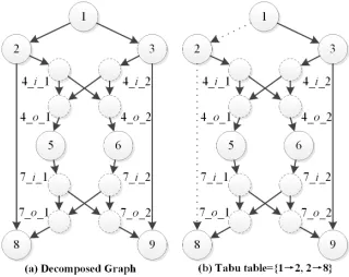
Fig. 2 illustrates an example of the graph decomposition method. The original graph with a source (i.e., node 1) and two receivers (i.e.,node8 andnode9) are shown in Fig. 2(a), wherenode4 andnode7 are merging nodes. Fig. 2(b) shows the decomposed graph, where eight auxiliary links are inserted. Node 4 is decomposed into two incoming auxiliary nodes, node4 i 1andnode4 i 2, and two outgoing auxiliary nodes, node4 o 1andnode4 o 2. Likewise,node7 is decomposed into four auxiliary nodes, as shown in Fig. 2(b). The decom-posed graph unveils all possibilities that information flows may pass through node4 and node7.
Note that each outgoing auxiliary node inGD(V0, E0)has a single outgoing link. Therefore, if more than one information flow joins an outgoing auxiliary node, it means the coding operation is required at that auxiliary node. In addition, the graph decomposition method only decomposes merging nodes which does not affect the source, receivers and data rate of the graph.
III. PROBLEM FORMULATION AND RELATED WORKS
A. Problem formulation
As aforementioned, a communication network is represent-ed by a directrepresent-ed graph G(V, E). After the graph
decomposi-Fig. 2. An example of the graph decomposition method
tion,G(V, E)is transformed to graphGD(V0, E0). A single-source network coding based multicast scenario can be defined as a 4-tuple set(GD, s, T, R), where the information needs to be transmitted at data rateR from the source node s∈V0 to a set ofd receivers T ={t1, t2, ..., td}. We assume each link has a unit capacity, so a path fromstotk has a unit capacity. IfRlink-disjoint paths{p1(s, tk), ..., pR(s, tk)}fromsto each
receivertk ∈T are set up, the data rateRis said to be achiev-able. The R link-disjoint path set {p1(s, tk), ..., pR(s, tk)} is
denoted by P aths(s, tk), where tk ∈ T. If we successfully obtained P aths(s, t1), ..., P aths(s, td), then we obtain a
feasible solution Solution(GD). According to the solution Solution(GD), a NCM subgraph can be built to support the multicast with network coding, which is denoted by GNCM(Solution(GD)).
The following lists some notations used in the paper:
• s: the source node inGD(V0, E0);
• T ={t1, t2, ..., td}: set of receivers, whered=|T|is the number of receivers;
• R: data rate (an integer) at whichsexpects to transmit to T;
• pi(s, tk): thei-th path from s to tk, where tk ∈ T and i=1, ...,R;
• Wi(s, tk): the set of links of pi(s, tk), i.e., Wi(s, tk) = {e|e∈pi(s, tk)};
• P aths(s, tk) ={p1(s, tk), ..., pR(s, tk)}: a path set from stotk, wheretk∈T and any two paths inP aths(s, tk) are link-disjoint;
• Solution(GD)={P aths(s, t1), ...,P aths(s, td)}: a
com-plete NCM solution;
• GNCM(Solution(GD)): a NCM subgraph that is built by
Solution(GD);
• OA(GD): the set of outgoing auxiliary nodes in GD(V0, E0);
• σo: a binary variable associated with each node o ∈ OA(GD). σo = 1 if at least two incoming links of nodeoare occupied byGNCM(Solution(GD));σo= 0, otherwise;
• ϕ(GNCM(Solution(GD))): the number of coding nodes inGNCM(Solution(GD)).
The NCRM problem is defined as to find a solution to build a NCM subgraph GNCM(Solution(GD))with the minimum
[image:3.612.356.517.56.184.2]satisfied, as shown below: Minimize:
ϕ(GNCM(Solution(GD))) =
X
∀o∈OA(GD)
σo (3)
Subject to:
R(s, tk) =R, ∀tk∈T (4)
Wi(s, tk)∩Wj(s, tk) =∅,
∀tk∈T, ∀i, j∈ {1, ..., R}, i6=j
(5)
Objective (3) defines the optimization problem as to mini-mize the number of coding operations. Constraint (4) defines that the achievable rate betweensand each receiver is exactly data rate R in solution Solution(GD), indicating there are R paths between the source and each receiver. Constraint (5) indicates that for arbitrary two paths fromstotk,pi(s, tk)and pj(s, tk)(i6=j), no common link exists so that each receiver can receive information at data rate R.
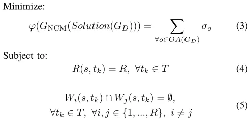
[image:4.612.56.299.68.185.2]An illustrative example is given in Fig. 3. Fig. 3(a) illustrates the decomposed graph for the original multicast scenario in Fig. 2. With data rate R=2 and two receivers, i.e.,node8 and node 9, we use an ant colony of two ant groups (AntG1and
AntG2) to address the NCRM problem, where each group
consists of two ants.AntG1 is responsible for finding a path
set of two link-disjoint paths from node1 to node8. AntG2
is for constructing a link-disjoint path set from node 1 to node9. Specifically, as shown in Fig. 3(b)-(c), the two ants in AntG1 find p1(1,8) = 1→2→8 andp2(1,8) = 1→3→
4 i 2 → 4 o 1 → 5 → 7 i 1 → 7 o 1 →8, respectively. Thus W1(1,8) = {1 → 2, 2 → 8} and W2(1,8) = {1 →
3, 3 → 4 i 2, 4 i 2→ 4 o 1, 4 o 1 →7 i 1, 7 i 1 → 7 o 1, 7 o 1→8}. Due toW1(1,8)∩W2(1,8) =∅, the two
pathsp1(1,8)andp2(1,8)are link-disjoint. Likewise, then the
other ants in AntG2 find two link-disjoint paths p1(1,9) =
1 →2→4 i 1→4 o 1 →5→7 i 1→7 o 2→9 and p2(1,9) = 1→ 3 →9, respectively. Eventually, a complete
solution Solution(GD) = {P aths(1,8), P aths(1,9)} can be constructed, where P aths(1,8) ={p1(1,8), p2(1,8)}and
P aths(1,9) ={p1(1,9), p2(1,9)}, then the associated NCM
subgraph is built as shown in Fig. 3(d). It is noted that node 4 o 1 is the only coding node in GNCM(Solution(GD)),
which means the number of the coding nodes ϕ equals to 1.
B. Related works
Due to the importance and the benefit network coding brings, the NCRM problem has received much attention re-cently. Fragouli et al. [24] and Langberg et al. [11] proposed two greedy-based approaches for solving the problem. How-ever, greedy algorithms do not perform well in escaping local optimum, leading to a deteriorated optimization performance when the link traversing order is not appropriate. Later on, Kim et al. [8]–[10] proved that the NCRM problem is NP-hard and carried out a series of research on how to efficiently apply genetic algorithms (GAs) to tackle the problem. Sim-ulation results demonstrate that GAs outperform the greedy
algorithms in a statistical manner. Since then, EA-based search algorithms have become the mainstream techniques for solving the NCRM problem in the field of computational intelligence. We classify the existing EAs into four categories by the individual encoding approaches adopted. EAs of the first category are based on the binary link state (BLS) encoding. As mentioned in Subsection II-B, for a merging nodem, there are |Im|×|Om|auxiliary links inserted between the corresponding incoming and outgoing auxiliary nodes. In BLS encoding, an individual consists of a number of binary variables, with each corresponding to the state of an auxiliary link (active or inactive). Hence, an explicit NCM subgraph can be built by a feasible individual. The BLS-based EAs include GAs [9], [10], [25], quantum-inspired EAs [26], [27], population based incremental learning [28], [29] and compact GA [30]. One of the disadvantages of BLS is that infeasible solutions account for the majority of the search space, which to a certain extent deteriorates the search ability and efficiency of EAs [31], [32]. EAs of the second category are based on the block transmis-sion state (BTS) encoding. BTS is similar to BLS. In BTS, an individual is divided into a number of blocks, each of which corresponds to an outgoing auxiliary node. If there are at least two 1’s in a block, the whole block is set to all-one block. In this way, the size of the search space is greatly decreased. Nevertheless, using BTS may lose useful information for guiding the search towards the global optima. GA [10] is based on BTS encoding. In addition, Ahn et al. incorporated the self-adaptive fitness assignment rule and entropy-based relaxation technique into EAs with BTS to improve the efficiency and effectiveness of the algorithms [33], [34].
As mentioned above, BLS and BTS encodings both record the explicit link states (active or inactive). But, the third category of the EAs utilizes the relative information of the flows [35]. To be specific, each link is associated with a coefficient which represents how the information is combined according to the combination of flows from the upstream links. Hu et al. invented this encoding approach and adapt several GAs, e.g., the ripple-spreading GA (RSGA) [36] and the spatial receding horizon control GA (SRHCGA) [37], for the problem in large-scale or complex networks. Meanwhile, a chemical reaction optimization (CRO) algorithm was studied for addressing the problem, with the operating principle in-spired from chemical reactions [38]. Different from optimizing routing only, their research also work out the associated information encoding/decoding scheme, which is an important and realistic issue when considering the practical deployment of NC.
The fourth stream of EAs is the path-oriented encoding method. Each individual is comprised by a union of paths from the source to one of the receivers. Compared with BLS and BTS, the path-oriented encoding results into a search space where all solutions are feasible. As there is no infeasible solution, the search space is well connected and the problem difficulty is reduced. Xing and Qu proposed a path-oriented encoding EA in [32].
Fig. 3. An illustrative example of the problem formulation
where coding cost, link cost, and quality-of-service indicators are often considered as multiple objectives for simultaneous optimization. Coding cost and link cost are often considered as two conflicting objectives in the context of MNCMRP. A number of multi-objective evolutionary algorithms have been proposed to gain the trade-off between the two costs [39]– [41]. Xing et al. formulated a novel MNCMRP, where the total cost and maximum end-to-end delay are two objectives [31]. The fast nondominated sorting genetic algorithm II (NSGA-II) was adapted for the problem. Moreover, Karunarathnea et al. investigated a MNCMRP with three objectives, including the number of coding nodes, the mean number of coding node input links and the sharing of resources by receivers [42].
IV. NCRM-ACO
In this section, we first describe the overall procedure of the ACO algorithm for the NCRM problem (NCRM-ACO), followed by details of the key mechanisms and significance of parameters in subsections.
A. Overall procedure of NCRM-ACO
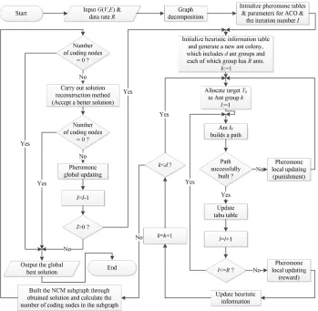
Fig. 4 is the overall procedure of NCRM-ACO and Fig. 5 shows the pseudo code of function PathSetConstruction. Fig. 6 shows the overall flow chart of the algorithm. In the proposed NCRM-ACO, first of all, with the original network G(V, E), the graph decomposition phase is executed so as to obtain a decomposed graph GD(V0, E0), based on which ACO is implemented to build feasible solutions. The proposed algorithm maintains a single ant colony at each generation. Within the colony, there are d ant groups AntGk, k=1, ..., d, each of which contains R ants (R is the expected data rate). Each ant group corresponding to one ofd receiver, i.e., the k-th ant group is in charge of finding a feasible path set P aths(s, tk) for receiver tk ∈ T, where P aths(s, tk) is composed of R link-disjoint paths from the source to tk. Each ant in AntGk finds a single path from the source to tk so that the above mentioned R link-disjoint paths are constructed for receiver tk. In the algorithm, d path sets are built one after another. If path setP aths(s, tk)is constructed successfully (see Subsection IV-D), it is used to update the pheromone and heuristic information of the ant colony to guide the path construction process (see Subsection IV-E).
With all path sets found, a complete solutionSolutionz(GD) consisting of all paths in these path sets is formed, where z is the generation number. Then, a NCM subgraph could be built by the solution and the number of coding nodes ϕ(GNCM(Solutionz(GD))) is easily calculated. After that, a solution reconstruction method is devised to improve the quality of Solutionz(GD) by exploring its neighboring area in the solution space, aiming to find an improved solution Solutionnew
z (GD) (see Subsection IV-F). Finally, the global (historical) best solutionSolutiongb(GD)obtained is used to update the pheromone so as to guide the search towards the optimal solution to the problem (see Subsection IV-G). The above process is repeated generation by generation, until the termination condition is met.
The pheromone and heuristic coefficients are two impor-tant coefficients, necessarily supporting effective search. In Subsections IV-B and IV-C, two problem-specific pheromone and heuristic maintenance mechanisms are described in detail. The remaining steps of NCRM-ACO are introduced from Subsections IV-D to IV-G.
B. The pheromone maintenance mechanism
In this paper, pheromone is used to provide essential guid-ance for the ant colony to gradually search towards the optimal solution for the NCRM problem. As mentioned in Subsection III-A, the less coding operations are required the better. Hence, pheromone is designed to be associated with the number of coding nodes a solution owns. This idea is similar to the pheromone scheme in TSP and 0-1 knapsack problems [14], [43], where pheromone is associated with the total distance and the total number of bins, respectively.
Input: A graphG, data rateR
1: Decompose graphGtoGD; . (Subsection II-B )
2: Initialize pheromone values; . (Subsection IV-B)
3: InitializeSolutiongb(GD) =∅;
4: whileTermination conditions NOT met do
5: Initialize Solutionz(GD) =∅;
6: Initialize heuristic information table; . (Subsection IV-C)
7: fork= 1toddo
8: InitializeP aths(s, tk) =∅;
9: SetP aths(s, tk)= PathSetConstruction(s, tk, R); . (Subsection IV-D)
10: whilesize ofP aths(s, tk)< Rdo
11: Invoke the pheromone local updating rule (punishment) to P aths(s, tk); .(Subsection IV-E)
12: SetP aths(s, tk)= PathSetConstruction(s, tk, R); . (Subsection IV-D)
13: end while
14: Invoke the pheromone local updating rule (reward) toP aths(s, tk); .(Subsection IV-E)
15: AddP aths(s, tk)into Solutionz(GD);
16: Update the heuristic information according toP aths(s, tk); . (Subsection IV-C)
17: end for
18: Apply solution reconstruction method to Solutionz(GD)and getSolutionnewz (GD); .(Subsection IV-F)
19: if ϕ(GNCM(Solutionnewz (GD)))< ϕ(GNCM(Solutiongb(GD))) then
20: Invoke pheromone global updating rule byϕ(GNCM(Solutionnewz (GD))); . (Subsection IV-G)
21: SetSolutiongb(GD) =Solutionnewz (GD);
22: end if 23: end while
[image:6.612.57.455.58.399.2]Output: The global best solutionSolutiongb(GD)andϕ(GNCM(Solutiongb(GD)))
Fig. 4. The overall procedure of NCRM-ACO
1: function PATHSETCONSTRUCTION(source, receiver, R)
2: Initialize P aths(source, receiver) =∅;
3: forl= 1 toR do
4: Antl builds a path from source toreceiver, denoted by pl(source, receiver); . (Subsection IV-D)
5: Addpl(source, receiver)into P aths(source, receiver);
6: end for
7: returnP aths(source, receiver); 8: end function
Fig. 5. The pseudo-code of constructing the path set from the source to a receiver
table is adopted, this conflicting and misleading information (pheromone overlapping problem) would not be able to pro-vide useful guidance for the solution construction procedure. This is because for an arbitrary link different ants may have different options on whether or not to occupy it.
In order to efficiently guide the search, NCRM-ACO uses a new pheromone maintenance mechanism employing multiple pheromone tables. We associate each ant in the ant colony with a pheromone table, leading to in totalR∗dpheromone tables, where R andd is the data rate and the number of receivers, respectively. Each table maintains the pheromone of an ant over the decomposed graph GD, where each auxiliary link is associated with a pheromone value. Let τ0 be the initial
pheromone value over each link. For all tables, τ0 is set to
a small positive number ϕmax= (|V0|)−1, where|V0|is the number of nodes in GD. Take Fig. 2(a) as an example, with d=2 andR=2, the NCRM-ACO maintains2×2 = 4pheromone tables as shown in Fig. 7. At different generations, those ants responsible for finding the same path, e.g.,p1(1,8), share the
same pheromone table. Moreover, τ0 for all links is set to
ϕmax = (|V0|)−1 = (15)−1. During the search procedure, the pheromone values in those tables are gradually updated, as introduced in Subsections IV-E and IV-G. The number of pheromone tables is the product of the number of the data rate Rand the number of receiversd. Data rateRis subjected by the max-flow from the source to a receiver. In the literature, data rateRis usually small. To the best of our knowledge, the largestRfor experiments and simulations is set to 7 [34]. So, the number of pheromone tables grows approximately linearly withd.
C. The heuristic maintenance mechanism
Fig. 6. The overall flow chat of NCRM-ACO
Fig. 7. An example of multiple pheromone tables maintained
problem aims to find a feasible routing subgraph consisting of multiple path sets, each of which contains a number of disjoint paths to the same receiver, where no clear heuristic information is immediately available.
In this paper, an efficient heuristic maintenance mechanism maintains how many times each link has been selected by different ant groups in the same generation. Heuristic infor-mation represents local inforinfor-mation and can provide some useful guidance when constructing the paths to form the NCM subgraph. According to Subsection II-B, an outgoing auxiliary node m ∈ OA(GD) will perform coding operations if the received information comes from more than one incoming link. How to reduce the probability of the incurrence of coding operations is desirable. Fortunately, the number of times that each incoming link is selected can help. This is because, at a
[image:7.612.51.299.438.525.2]phase.
In the proposed mechanism, the heuristic information is maintained in one table, called Key-Value map, where Key and Value represent the link ID and its corresponding value, respectively. The value stands for the number of times a link has been selected. Initially, the value of each link is set to 1. All path sets are constructed in a one-by-one manner. The table is updated after each of thedpath sets is constructed by adding a value of 1 to the heuristic information value of each link in the path set. At the beginning of each new generation, the values of all links are reset to 1 since the heuristic information is only used to indicate the link occupation status of the incumbent generation.
D. Tabu-table based path construction
Different from the TSP, the NCRM problem is much more complex. It aims to construct multiple path sets, with each consisting of a number of link-disjoint paths from the source to a certain receiver. Due to the problem nature, it is often possible that an ant could not reach its destination, e.g., receivertk. To overcome this problem, we propose a tabu-table based path construction method to increase the probability that an arbitrary ant can find a feasible and demanded path.
In the proposed method, the route of each ant starts from the source and ends up with one of the receivers. A feasible solution to the NCRM problem is quite difficult to construct, since one needs to find multiple path sets, where each path set contains multiple link-disjoint paths from the source to the same receiver. To ease the above problem, for each ant group AntGk, we maintain a tabu table to record which links have been employed. Those employed links will not be visited by other ants within AntGk. Fig. 8 illustrates a simple example of the tabu table. When ant1 inAntG1 find p1(1,8) = 1→
2→8 as shown in Fig. 8(b), the two links1→2and2→8 are added in the tabu table. Then, ant2 of AntG1 would not
choose the two links any more. If there is only a single link from node i, the ant will move to this link; otherwise, those available links Ψi which are not being included in the tabu table will have a chance to be selected. To select a link from Ψi, the pseudo-random rule [14] is adopted to calculate the probability by formula (6).
np=
(
arg max u∈Ψi
[τ(tk, l,(i, u))] α
[η(i, u)]β ,if q≤q0
ζ ,otherwise
(6)
where argument τ(tk, l,(i, u)) is amount of pheromone and η(i, u)is the amount of heuristic information on link (i, u). In τ, receivertk and path number lare both associated with the pheromone maintenance mechanism. Parameters α and β define the relative importance of the pheromone and the heuristic information, respectively.qis a uniformly distributed random number in the range [0,1] and q0(0<q0<1) is a
threshold value. ζ is a random value determined by the probability of p(i, j)ifq is greater thanq0:
p(i, j) =
[τ(tk,l,(i,j))]α[η(i,j)]β
P
u∈Ψi
[τ(tk,l,(i,u))]α[η(i,u)]β
, j∈Ψi
0,otherwise
[image:8.612.357.517.56.183.2](7)
Fig. 8. An example of the tabu table
By using formulae (6) and (7), each ant may either follow the most favorite path already established or randomly select a path based on the probability distribution of the pheromone and the heuristic accumulated. It is noted that the pseudo-random rule facilitates the diversity of the stochastic search and hence it helps to enhance the global search ability.
E. The pheromone local updating rule
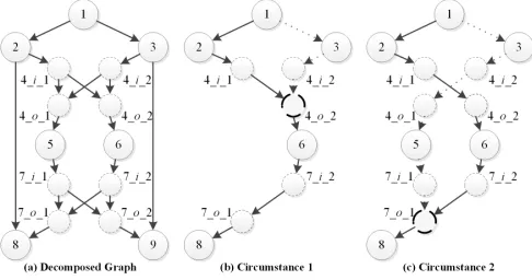
The expected data rate R, as a hard constraint, must be satisfied during the establishment of the network coding based multicast session. This can be achieved by constructingR link-disjoint paths from the source to each receiver. However, even if the tabu table scheme is employed, an infeasible path could be resulted if an ant chooses inappropriate links. Take Fig. 9(a) as an example. An ant in ant groupAntG1 has constructed a
pathp1(1,8) = 1→2 →4 i 1→4 o 1 →5→7 i 1 →
7 o 1 → 8 from source node 1 to receiver node 8 and all links in p1(1,8) are recorded in the tabu table. The other
ant in AntG1 cannot construct a second path p2(1,8) that
is link-disjoint with p1(1,8) from node 1 to node 8 in any
circumstance, as shown in Figures 9 (b) and (c). Apparently, if this happens, we could send a new group of ants to reconstruct a feasible path set. In NCRM-ACO, a pheromone punishing-and-rewarding mechanism is proposed to avoid ants following the same paths as the old group does.
In the pheromone punishing scheme, if an ant groupAntGk fails to construct a feasible path set, e.g., P aths(s, tk), the pheromone values on those paths which have been employed by AntGk are decreased by a constant ∆τloc before the reconstruction ofP aths(s, tk)as follows.
τ(tk, l,(i, j)) =τ(tk, l,(i, j))−∆τloc (8)
where the value ∆τloc is a small positive number. In the pheromone local updating rule,∆τloc= (ϕmax)−1.
Fig. 9. An example of the inappropriate path selection
On the contrary, in the pheromone rewarding scheme, when a feasible path set is constructed successfully, the associated ant group will be rewarded by means of increasing the pheromone values on links they employ by∆τlocat each time (see formula (9)).
τ(tk, l,(i, j)) =τ(tk, l,(i, j))+∆τloc (9)
In summary, the pheromone local updating rule is composed of the punishing and rewarding schemes to guide the construc-tion of feasible soluconstruc-tions.
F. Solution reconstruction method
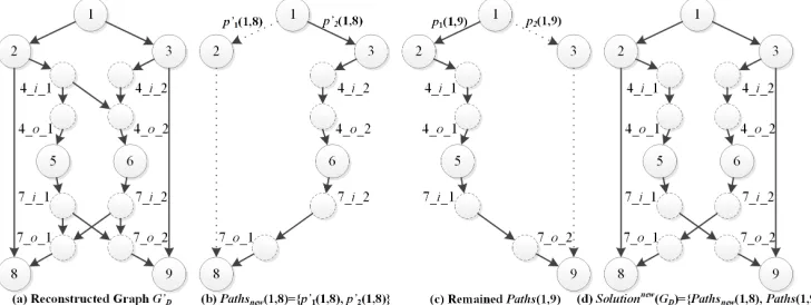
It is widely recognized that prematurity often happens in ACO and could cause serious performance deterioration [15], [44]. Hence, we develop a solution reconstruction method to improve the quality of the solution obtained, aiming at enhanc-ing the local exploitation ability and avoidenhanc-ing the premature convergence. The solution reconstruction method consists of three steps. First of all, for a given solution Solution(GD), we randomly select a coding nodemcoding from it. Secondly, we randomly select one of the incoming links, e.g., ecoding, of node mcoding. Then, we divide all path setsP aths(s, tk), k = 1, ..., d, of Solution(GD) into two groups, i.e., unaf-fectedPaths and affectedPaths. Assume there are h path sets in affectedPaths, where h is a positive integer smaller than the number of receivers d. So unaffectedPaths contains (d -h) path sets. P aths(s, tk) is included into affectedPaths if link ecoding ∈P aths(s, tk); otherwise, P aths(s, tk) belongs to unaffectedPaths. Thirdly, we reconstruct all path sets in affectedPaths, with unaffectedPathsunchanged. After that, all path sets inunaffectedPathsandaffectedPathsare combined to form a new solution, aiming to reduce the coding operations involved.
The path set reconstruction is described below. First, with link ecoding unchanged, we delete the rest of the incoming links of node mcoding from GD resulting into a new graph G0D. Then, we send h ant groups to rebuild all path sets in affectedPaths over G0D. Note that, it is possible that graph G0D cannot meet the data rate requirement after the deletion of those incoming links. So, when rebuilding a path set, e.g., P aths(s, tk), we limit the number of times attempt-ed. If the reconstruction cannot be completed after these attempts, NCRM-ACO gives up the reconstruction process;
in P aths(1,9) but not in P aths(1,8), we have unaffected-Paths={P aths(1,9)}andaffectedPaths={P aths(1,8)}. After that, apart from link e, the rest of the incoming links of node 4 o 1, i.e., link node 4 i 2 →node4 o 1, is deleted from the graph, and the reconstruction of P aths(1,8) is triggered. Fig. 10(a) shows the new graph G0D after the deletion of incoming links. Suppose the new ant group successfully constructs two link-disjoint paths, p01(1,8) = 1 → 2 → 8 and p02(1,8) = 1 → 3 → 4 i 2 → 4 o 2 → 6 → 7 i 2 → 7 o 1 → 8. We thus have P athsnew(1,8) ={p0
1(1,8), p02(1,8)}, as shown in Fig. 10(b).
Then, a new solution is formed by combiningP athsnew(1,8) and P aths(1,9), with no coding operation required (see Fig. 10(d)). Due to ϕ(GNCM(Solutionnew(GD))) < ϕ(GNCM(Solution(GD))), we replace the old solution with Solutionnew(G
D).
G. The pheromone global updating rule
In addition to the pheromone local updating rule, NCRM-ACO adopts a pheromone global updating rule to guide the search towards optimal solutions. Under this rule, the pheromone information on all links is updated by a historic best solution Solutiongb(GD), providing some instructive guidance to improve the quality of the solutions built. The pheromone value is updated by using formulae (10) and (11).
τ(tk, l,(i, j)) = (1−ρ)τ(tk, l,(i, j)) +ρ∆τgb (10)
∆τgb=
(ϕgb)−1,if (i, j)∈Solutiongb(GD)
0, otherwise (11)
where parameterρ∈(0,1]is a constant value, called the evap-oration rate, mimicking the evapevap-oration of the pheromone on all links [21], i.e., the pheromone value on each link decreases byρwhenever the global pheromone updating is executed.ϕgb is the number of coding nodes inGNCM(Solutiongb(GD)).
V. PERFORMANCE EVALUATION
Fig. 10. An example of the solution reconstruction method
A. Test instances
We evaluate the performance of the proposed algorithm on 35 benchmark instances which can be classified into four categories, namely, Fixed, Random, Hybrid and Real-world networks. Table I shows all instances and their parameters. To encourage future scientific comparison on the NCRM problem, these instances are available at http://www.cs.nott.ac.uk/∼rxq/
benchmarks.htm. All experiments are run on a computer with Windows 8 OS, Intel(R) Core(TM) i7-3740QM CPU 2.7 GHz and 8 GB RAM.
• Fixed networks.These four networks have been widely used in the literature [8]–[10], [26]–[30], [32]–[38]. They are also referred to as n-copy networks, each of which is built by cascading n copies of Basic network (a) (see Fig. 11(a)). Fig. 11(c) illustrates the 3-copy network, where node 1 is the source and nodes 16, 17, 24, 25 are receivers. It can be easily inferred that the minimum number of the coding operations to anyn-copy networks is 0.00.
• Random networks. Networks of this type are all gen-erated by the directed acyclic graph generation method introduced in [45]. The 18 random networks have 20 to 500 nodes. It is noted that Rnd-11 to Rnd-18 are relatively large networks.
• Hybrid networks. Due to that all test cases have the global minimum of 0.00, we generated 8 hybrid networks, where the global minimum of each instance is at least 1 and is known beforehand. This is done by combining two basic networks together, i.e., Fig. 11(a) and Fig. 11(b), where Fig. 11(a) is coding-free while Fig. 11(b) has an explicit coding node, i.e., node 4. In this way, a hybrid network can be built by combining a number of Fig. 11(a) and Fig. 11(b) networks together. The global minimum of an instance is equal to the number of Fig. 11(b) networks. Therefore, in hybrid networks, the global minimum is already known. The hybrid networks are called X-hybrid(Y), where X represents the number of networks being combined and Y indicates the global minimum value. Similar to the 3-copy, 7-copy, 15-copy and 31-copy networks, we create 3-hybrid, 7-hybrid, 15-hybrid, and 31-hybrid networks, respectively. The global minimum is from 1 to 5. Fig. 11(d) illustrates 3-hybrid(1)
network which contains two Fig. 11(a) networks and one Fig. 11(b) network. The global minimum is 1. Therefore, hybrid networks could be used to simulate networks where coding is necessarily performed and reflect the optimization ability of the algorithm in solving this type of the NCRM problem.
• Real-world networks. Five real-world topologies have
[image:10.612.313.567.374.527.2]been adopted for the performance evaluation, namely, Ebone-1, Ebone-2, Ebone-3, Exodus-1, and Exodus-2 [33], [34]. We also use them in our experiments.
Fig. 11. A example of fixed and hybrid networks
(a) Basic network 1; (b) Basic network 2; (c) 3-copy; (d) 3-hybrid(1)
B. Performance measures
To thoroughly evaluate the performance of the proposed algorithm, the following performance measuring metrics are employed throughout the experiments.
• Mean and Standard Deviation (SD) of the best solutions
found from 50 runs. Mean and SD are important met-rics to demonstrate the overall performance of a search algorithm.
• Average Computational Time (ACT) consumed by an algorithm over 50 runs. This metric is a direct indication of the computational time of an algorithm.
Random Rnd-8 50 118 10 4 4.72 194 307 189 0
Rnd-9 60 150 11 5 5.00 239 385 235 0
Rnd-10 60 156 10 4 5.20 262 453 297 0
Rnd-11 100 175 10 2 3.50 245 389 214 0
Rnd-12 100 279 10 3 5.58 433 879 600 0
Rnd-13 150 337 16 2 4.49 483 851 514 0
Rnd-14 150 363 11 3 6.17 712 1519 1056 0
Rnd-15 200 527 18 2 5.27 823 1586 1059 0
Rnd-16 200 473 12 3 4.73 703 1272 799 0
Rnd-17 500 1086 33 2 4.34 1682 2947 1861 0
Rnd-18 500 491 24 3 5.46 2187 4413 3048 0
Hybrid
3-hybrid(1) 24 34 4 2 2.83 42 58 24 1
3-hybrid(2) 23 32 4 2 2.78 35 48 16 2
7-hybrid(2) 55 80 8 2 2.91 107 148 68 2
7-hybrid(3) 54 78 8 2 2.89 102 140 62 3
15-hybrid(3) 118 174 16 2 2.95 238 332 158 3
15-hybrid(4) 117 172 16 2 2.94 233 324 152 4
31-hybrid(4) 245 364 32 2 2.97 505 708 344 4
31-hybrid(5) 244 362 32 2 2.97 500 700 338 5
Real world
Ebone-1 18 23 5 2 2.44 31 39 16 0
Ebone-2 31 45 5 3 2.90 58 80 35 0
Ebone-3 26 45 5 4 3.46 62 99 54 0
Exodus-1 24 30 5 2 2.50 37 46 16 0
Exodus-2 33 51 5 3 2.73 71 105 54 0
with 98 degrees of freedom at a 0.05 level of significance is used. The t-test result can show statistically if the performance of A is better than, worse than, or equivalent to that of B.
C. Parameter settings
The performance of the proposed ACO could be seriously deteriorated, e.g., leading to slow convergence and prematurity, if the values of parameters, namely, the pheromone factor α, the heuristic factor β, the pheromone evaporation rate ρ and the pseudo-random coefficient q0, are inappropriately
set. In order to determine an appropriate combination of the parameter values, for each parameter, we tested 4 pos-sible values, i.e., α ∈ {0.6,0.7,0.8,0.9}, β ∈ {2,3,4,5}, ρ ∈ {0.0,0.1,0.2,0.3} and q0 ∈ {0.4,0.5,0.6,0.7}. This
may lead to 44 = 256 combinations if we try all possible
parameter values. However, it is not necessary to try all the combinations, since we only want to determine an appropriate combination, rather than the best setting. We thus use the orthogonal experimental design (OED) to find a relatively better combination. OED is a multi-parameter experimental design method based on orthogonal array, where a number of representative combinations of parameter values which are uniformly distributed within the test range are selected from the full parameter experiment [47]. This method is highly efficient when designing multi-parameter experiments. It can greatly reduce the number of required experiments while obtaining promising results. Since its introduction in 1950s,
OED has been widely applied in many areas, such as economic management, bioengineering, environmental engineering, etc. [48]–[50]. The following briefly introduces the procedure of OED.
Let La(bc) denote the orthogonal array, where a is the number of experiments, b is the levels of parameters, and c is the number of parameters. The orthogonal array has two properties, i.e., (1) in each column, the number of occurrences of different numbers is equal and (2) in any two columns, the arrangement of numbers is complete and balanced. Any parameter at each level is thus compared to all different parameters with each other. Consequently, test results can be analyzed through range and variance analysis to determine a better value combination of parameters. More details can be found in [47]–[51]. In our experiment, an orthogonal array L16(44) is obtained from the referencing orthogonal table,
where 16 representative combinations are listed in Table II. We carry out 50 independent runs for each parameter com-bination and record the mean value of the best solutions. As Fix-4 network instance is one of the most difficult instances, we use it to run the parameter settings experiments.
Table III shows the Mean values of the 16 combinations in Table II. It is noted that row m1 to row m4 represent
the mean value of a certain parameter with a certain value. For instance, the mean value of parameterα=0.6 is calculated as (6.82+5.78+0.60+1.28)/4=3.62. So, value 3.62 is recorded in row m1, column α. Moreover, the mean value of each
TABLE II
TABLE OF ORTHOGONAL ARRAYL16(44)
ParaCom α β ρ q0 ParaCom α β ρ q0
1 1 1 1 1 9 3 1 3 4
2 1 2 2 2 10 3 2 4 3
3 1 3 3 3 11 3 3 1 2
4 1 4 4 4 12 3 4 2 1
5 2 1 2 3 13 4 1 4 2
6 2 2 1 4 14 4 2 3 1
7 2 3 4 1 15 4 3 2 4
8 2 4 3 2 16 4 4 1 3
Note: numberxin the columnsα,β,ρ,q0correspond to thex-th
value in the parameter value set
TABLE III
RESULTS OF THE ORTHOGONAL EXPERIMENTAL DESIGN
ParaCom α β ρ q0 Mean
1 0.6 2 0.0 0.4 6.82
2 0.6 3 0.1 0.5 5.78
3 0.6 4 0.2 0.6 0.60
4 0.6 5 0.3 0.7 1.28
5 0.7 2 0.1 0.6 0.56
6 0.7 3 0.0 0.7 4.40
7 0.7 4 0.3 0.4 0.62
8 0.7 5 0.2 0.5 1.16
9 0.8 2 0.2 0.7 1.04
10 0.8 3 0.3 0.6 0.00
11 0.8 4 0.0 0.5 0.64
12 0.8 5 0.1 0.4 1.18
13 0.9 2 0.3 0.5 2.86
14 0.9 3 0.2 0.4 1.62
15 0.9 4 0.1 0.7 0.44
16 0.9 5 0.0 0.6 1.84
m1 3.62 2.82 3.43 2.56 /
m2 1.69 2.95 1.99 2.61 /
m3 0.72 0.58 1.11 0.75 /
m4 1.69 1.37 1.19 1.79 /
Note: The symbol / means not applicable
and q0=0.6, NCRM-ACO achieves the smallest mean value.
Then, we compare the optimization performance of two com-binations, i.e. {0.8,4,0.2,0.6} and {0.8,3,0.3,0.6} which gains the minimum mean value in Table II. In this experiment, performance indicators Mean and ACT are used and the results are shown in Table IV. It is seen that each combination obtains a mean value of 0.00, indicating both of them can achieve the optimal solution in each single run. However, in terms of the ACT, ACO with {0.8,4,0.2,0.6} is faster. It is hence clear that the first combination in Table IV performs the best and is hereafter used as the parameter settings.
● ● ● ● α Mean
0.60 0.70 0.80 0.90
0 1 2 3 4 ● ● ● ● β 2.0 3.0 4.0 5.0
●
●
● ●
ρ 0.00 0.10 0.20 0.30
● ●
● ●
q0 0.40 0.50 0.60 0.70
Fig. 12. Relationship between average time and parameters
TABLE IV
RESULTS OF ADDITIONAL EXPERIMENTS
ParaCom α β ρ q0 Mean ACT (sec.)
1 0.8 4 0.2 0.6 0 14.84
2 0.8 3 0.3 0.6 0 18.72
D. Effectiveness of the proposed mechanisms
We evaluate the effectiveness of the proposed mechanisms by implementing two experiments on 14 selected instances, including the four fixed networks (3-copy, 7-copy, 15-copy, 31-copy) and ten random networks (Rnd-1, ..., Rnd-10), be-cause these instances have been widely used for performance evaluation.
The proposed ACO is featured with five specially devised mechanisms, including the multi-dimensional pheromone maintenance mechanism, the problem-specific heuristic infor-mation, the tabu-table based path construction, the pheromone local updating rule and the solution reconstruction method (see Section IV for details). Among them, the first two are essential components to drive ACO run properly. In other word, they are fundamental mechanisms that adapt ACO for the NCRM problem. One cannot test the effectiveness of the pheromone maintenance and the heuristic information in a separate way. Hence, we evaluate the two mechanisms as a whole (the first experiment) and test the others independently (the second experiment). The algorithms for comparison are listed below.
• Exp1:Verification of the first two mechanisms
– A1:the basic ACO [23]
– A2:A1 with the multi-dimensional pheromone main-tenance mechanism and the problem-specific heuris-tic information (see Subsections IV-B and IV-C);
• Exp2:Independent verification of the rest mechanisms
– A3: A2 with the tabu-table based path construction (see Subsection IV-D);
– A4:A2 with the pheromone local updating rule (see Subsection IV-E);
– A5: A2 with the tabu-table based path construction and the pheromone local updating rule;
– A6:A2 with the solution reconstruction method (see Subsection IV-F);
– A7: A1 with all proposed mechanisms (also called NCRM-ACO).
As there is no clear heuristic information immediately available, we set heuristic information factor β of A1 to 0. For A2 to A7, we setβ = 4, with which the algorithm could achieve better optimization performance, as demonstrated in Subsection V-C.
[image:12.612.52.290.600.730.2]other hand, with the proposed pheromone maintenance mech-anism and the heuristic information utilized, A2 is successfully applied to the NCRM problem.
Then, we compare A3, ..., A6 with A2 to verify if each of the three mechanisms has a positive impact on the performance of A2. Due to the nature of the NCRM problem, it is extremely difficult to find a satisfied set of link-disjoint paths. Hence, even with the pheromone maintenance mechanism and heuris-tic information integrated, it is still possible that an ant cannot reach its destination. In order to enhance the ability for an arbitrary ant to find a demanded path and diversify link-disjoint path sets, the tabu-table based path construction is developed. It can be seen that A3 outperforms A2 in all instances in terms of Mean value. Meanwhile, even if the tabu-table based path construction is used, it is still possible to result into an infea-sible path if inappropriate links are chosen. So, we need the pheromone local updating rule as a complement to the tabu-table based path construction. If we compare the performance of A4 and A2, we see that the former is better. This is because, by using the punishing and rewarding schemes, the pheromone local updating rule is able to avoid ants following the same paths as the previous group does, which helps to improve the optimization performance. Meanwhile, by comparing the performance of A5, A4 and A3, we can verify the effectiveness of the tabu-table based path construction and the pheromone local updating rule. Clearly, the two mechanisms perform better than any of them individually adopted. If looking at the results of A6 and A2, we also observe that the former performs better than the latter. The reason is explained below. As aforementioned, ACO may suffer from the prematurity. The solution reconstruction mechanism can improve the quality of solutions, so the local exploitation is enhanced and the local optimum can be avoided.
Finally, A7 is compared with A2, ..., A6. Obviously, A7 always obtain optimum in any of the instances. Regarding the mean and SD, it performs no worse, but usually better than the others. This demonstrates that equipped with all specially-devised mechanisms, the proposed algorithm has a significantly improved optimization performance.
According to the above comparisons, we see that each of the proposed mechanisms contributes to the improvement of the NCRM-ACO. To further support our findings, we compare the seven algorithms using Student’s t-test, where results are given in Table VI. The result of A↔B is shown as ‘+’, ‘-’, or ‘∼’ when algorithm A is significantly better than, significantly worse than, or statistically equivalent to algorithm
[28] and cGA [30]), 2 BTS-based (BTSGA [10] and FA-ENCA [34]), 3 relative-encoding-based (RGA [35], SRHCGA [37] and CRO [38]), and 1 path-oriented (pEA [32]). The algorithms for performance comparison are listed as follows.
• BLSGA:BLS encoding-based GA [10].
• QEA1:Quantum-inspired evolutionary algorithm (QEA) [27].
• QEA2:Another QEA proposed by Ji and Xing [26].
• PBIL: Population-based incremental learning algorithm [28].
• cGA:Compact genetic algorithm [30].
• BTSGA:BTS encoding-based GA [10].
• FA-ENCA: Fast and adaptive evolutionary algorithm [34].
• RGA:GA proposed by Hu et al [35].
• SRHCGA: Spatial receding horizon control (SRHC)
genetic algorithm [37].
• CRO:Chemical reaction optimization algorithm [38]. • pEA:the path-oriented encoding EA [32].
• NCRM-ACO:the proposed algorithm.
The population size is set to 20 and the maximum number of generations is 200 for each EA. For BLSGA, we set the crossover probabilitypc= 0.8 and the mutation probabilitypm = 0.006. For BTSGA, we havepc=0.8 andpm= 0.012. For the rest of the algorithms, we adopt their best parameter settings [26], [27], [29], [30], [32], [34], [35], [37], [38] . For the fixed, random and real-world networks, the stopping criteria is either an optimal solution is obtained or the maximum number of generations is reached. For the hybrid networks, an algorithm stops when either the best-so-far solution has not been changed over 20 generations or the maximum number of generations is reached. The results of Mean and SD are collected in Table VII, where the value should read Mean(SD). Tables VIII and IX illustrate the t-test results and the ACTs of the 12 algorithms.
TABLE V
RESULTS OF MEAN(SD) (BEST RESULTS ARE IN BOLD)
Network Exp1 Exp2
A1 A2 A3 A4 A5 A6 A7
3-copy / 0(0) 0(0) 0(0) 0(0) 0(0) 0(0)
7-copy / 1.62(1.50) 0.44(0.54) 0.48(0.62) 0.10(0.30) 0.86(0.72) 0(0) 15-copy / 7.52(1.90) 4.72(1.08) 5.16(1.16) 4.54(1.19) 6.10(1.13) 0(0) 31-copy / 21.84(5.67) 14.08(2.74) 15.18(2.52) 14.60(2.25) 18.90(2.62) 0(0) Rnd-1 / 0.14(0.35) 0(0) 0.02(0.14) 0(0) 0(0) 0(0)
Rnd-2 / 0(0) 0(0) 0(0) 0(0) 0(0) 0(0)
Rnd-3 / 0.28(0.43) 0(0) 0.06(0.24) 0(0) 0(0) 0(0) Rnd-4 / 0.52(0.90) 0(0) 0.08(0.27) 0(0) 0(0) 0(0) Rnd-5 / 1.50(1.27) 1.28(0.76) 1.38(1.31) 0.34(0.65) 0.26(1.22) 0(0) Rnd-6 / 0.06(0.24) 0(0) 0(0) 0(0) 0(0) 0(0) Rnd-7 / 2.06(2.12) 0.76(0.48) 0.92(0.72) 0.54(0.50) 0.36(0.97) 0(0) Rnd-8 / 2.72(2.53) 1.66(0.79) 1.92(1.34) 0.56(1.00) 0.24(0.81) 0(0) Rnd-9 / 5.40(4.98) 1.36(1.38) 1.84(0.76) 0.46(1.19) 3.08(2.97) 0(0) Rnd-10 / 2.92(2.04) 1.72(0.86) 2.04(1.22) 0.68(1.07) 1.54(1.82) 0(0)
Note: The symbol / stands for that the algorithm can’t find any feasible solution
TABLE VI
t-TEST RESULTS OF THE SEVEN ALGORITHMS
Network A2↔A1 A3↔A2 A4↔A2 A5↔A2 A6↔A2 A7↔A2 A5↔A3 A5↔A4 A7↔A5 A7↔A6
3-copy + ∼ ∼ ∼ ∼ ∼ ∼ ∼ ∼ ∼
7-copy + + + + + + + + + +
15-copy + + + + + + + + + +
31-copy + + + + + + ∼ + + +
Rnd-1 + + + + + + ∼ + ∼ ∼
Rnd-2 + ∼ ∼ ∼ ∼ ∼ ∼ ∼ ∼ ∼
Rnd-3 + + + + + + ∼ + ∼ ∼
Rnd-4 + + + + + + ∼ + ∼ ∼
Rnd-5 + + + + + + + + + +
Rnd-6 + + + + + + ∼ ∼ ∼ ∼
Rnd-7 + + + + + + + + + +
Rnd-8 + + + + + + + + + +
Rnd-9 + + + + + + + + + +
TABLE VII
RESULTS OFMEAN ANDSD (BEST RESULTS ARE IN BOLD)
Network BLSGA QEA1 QEA2 PBIL cGA BTSGA FA-ENCA RGA SRHCGA CRO pEA NCRM-ACO
3-copy 0.52(0.84) 0(0) 0(0) 0(0) 0(0) 0(0) 0(0) 0(0) 0(0) 0(0) 0(0) 0(0)
7-copy 2.36(2.22) 0.30(0.65) 0.74(1.18) 0(0) 0(0) 0.38(0.41) 0(0) 0(0) 0(0) 0(0) 0(0) 0(0)
15-copy 10.44(7.02) 2.82(3.31) 5.92(1.86) 1.76(2.57) 0(0) 0.08(0.22) 0.15(0.23) 0(0) 0.04(0.55) 0.10(0.41)0(0) 0(0)
31-copy 31.66(6.48) 16.68(8.80) 20.02(0.22) 22.74(8.43) 0(0) 8.58(3.42) 20.35(3.90) 0.03(0.44) 0.01(0.14) 0.26(0.59)0(0) 0(0)
Rnd-1 0.74(1.20) 0.12(0.31) 0.10(0.31) 0(0) 0(0) 0.28(0.44) 0(0) 0.01(0.14) 0.44(0.50) 0.20(0.40)0(0) 0(0)
Rnd-2 0.26(0.64) 0(0) 0(0) 0(0) 0(0) 0.02(0.22) 0(0) 0(0) 0.16(0.37) 0.06(0.47)0(0) 0(0)
Rnd-3 0.24(0.68) 0(0) 0(0) 0(0) 0(0) 0(0) 0(0) 0(0) 0.08(0.27) 0.18(0.48)0(0) 0(0)
Rnd-4 0(0) 0(0) 0(0) 0(0) 0(0) 0(0) 0(0) 0(0) 0(0) 0(0) 0(0) 0(0)
Rnd-5 1.42(0.88) 0.46(0.51) 0.38(0.41) 0(0) 0.12(0.36) 0.38(0.57) 0(0) 0.50(0.50) 0.58(0.58) 0.96(0.52)0(0) 0(0)
Rnd-6 0.22(0.41) 0(0) 0(0) 0(0) 0(0) 0(0) 0(0) 0.06(0.47) 0.46(0.81) 0.48(0.59)0(0) 0(0)
Rnd-7 1.38(0.97) 0.72(0.57) 0.62(0.48) 0.28(0.41) 0.56(0.58) 0.58(0.51) 0(0) 0.80(1.41) 0.12(0.69) 1.70(1.42)0(0) 0(0)
Rnd-8 2.54(2.08) 0.78(0.85) 0.72(0.71) 0.32(0.31) 0.38(0.51) 0.92(0.56) 0(0) 1.40(1.56) 0.50(1.03) 2.10(1.53)0(0) 0(0)
Rnd-9 2.76(1.25) 1.58(1.05) 1.58(0.99) 0(0) 0.12(0.41) 0.88(0.63) 0(0) 1.26(0.76) 0.72(0.72) 2.54(1.53)0(0) 0(0)
Rnd-10 3.18(2.67) 0.48(0.68) 0.28(0.47) 0.04(0.22) 0.08(0.22) 0.96(0.59) 0(0) 1.78(1.96) 0.52(0.76) 2.82(2.33)0(0) 0(0)
Rnd-11 0(0) 0(0) 0(0) 0(0) 0(0) 0(0) 0(0) 0(0) 0(0) 0.12(0.33)0(0) 0(0)
Rnd-12 0.28(0.57) 0(0) 0(0) 0(0) 0(0) 0.24(0.44) 0(0) 0.52(0.50) 0.14(0.35) 0.64(0.48)0(0) 0(0)
Rnd-13 25.32(25.30) 0.02(0.22) 0(0) 0(0) 0(0) 0.18(0.37) 0(0) 0.48(0.59) 0.16(0.73) 0.68(1.07)0(0) 0(0)
Rnd-14 25.20(25.45) 0(0) 0(0) 0(0) 0(0) 0.14(0.37) 0(0) 0.22(0.41) 0.30(1.01) 0.78(0.97)0(0) 0(0)
Rnd-15 0.16(0.37) 0.02(0.22) 0.20(0.52) 0(0) 0(0) 0.08(0.22) 0(0) 0.36(0.72) 0.90(1.92) 0.60(0.80)0(0) 0(0)
Rnd-16 2.34(1.35) 1.30(0.92) 1.48(0.89) 0.40(1.57) 0(0) 1.24(0.91) 0(0) 1.90(1.37) 1.48(1.15) 2.54(1.98)0(0) 0(0)
Rnd-17 1.72(1.42) 0.84(0.90) 1.01(0.47) 1.08(0.29) 0(0) 1.40(0.75) 0.20(0.40) 5.68(6.01) 5.38(3.85) 7.14(4.15)0(0) 0(0)
Rnd-18 8.26(2.59) 2.04(0.90) 1.18(0.37) 1.20(0.40) 0(0) 9.50(1.24) 1.30(1.08) 10.20(2.34) 7.38(1.49) 12.45(3.35)0(0) 0(0)
3-hybrid(1) 1.16(0.37) 1(0) 1(0) 1.16(0.49) 1(0) 1.04(0.22) 1(0) 1(0) 1(0) 1(0) 1(0) 1(0)
3-hybrid(2) 2.22(0.44) 2(0) 2(0) 2(0) 2(0) 2(0) 2(0) 2(0) 2(0) 2(0) 2(0) 2(0)
7-hybrid(2) 3.66(1.39) 2.10(0.31) 3(2.13) 2.54(1.23) 2(0) 2.40(0.60) 2.10(0.30) 2(0) 3.20(1.79) 2.10(0.30)2(0) 2(0)
7-hybrid(3) 4.98(2.48) 3.10(0.31) 3.60(1.85) 3.88(1.84) 3(0) 3.22(0.44) 3.34(2.24) 3(0) 3.50(1.09) 3.34(2.24)3(0) 3(0)
15-hybrid(3) 10.70(5.44) 6.20(4.49) 8.44(3.80) 5.76(3.85) 3.70(0.47) 4.72(0.92) 4.64(1.38) 7.32(3.47) 5.46(4.82) 8.30(3.67)3(0) 3(0)
15-hybrid(4) 11.12(4.88) 10.90(8.33) 8.80(4.16) 7.34(4.83) 4(0) 5.30(1.08) 5.64(2.58) 9.48(3.58) 5.72(4.50) 9.64(3.46)4(0) 4(0)
31-hybrid(4) 37.00(9.27) 31.70(13.26)28.06(8.94)37.10(10.90) 4(0) 10.90(2.64)10.20(1.56)30.80(7.95)26.80(11.93)35.80(9.18)4(0) 4(0)
31-hybrid(5) 32.80(8.12) 30.94(14.90)28.20(3.88)29.60(11.82) 5(0) 10.90(1.29) 9.80(3.23) 33.40(7.18)25.50(12.38)36.20(8.92)5(0) 5(0)
Ebone-1 0(0) 0(0) 0(0) 0(0) 0(0) 0(0) 0(0) 0(0) 0(0) 0(0) 0(0) 0(0)
Ebone-2 0(0) 0(0) 0(0) 0(0) 0(0) 0(0) 0(0) 0(0) 0(0) 0(0) 0(0) 0(0)
Ebone-3 0(0) 0(0) 0(0) 0(0) 0(0) 0(0) 0(0) 0(0) 0(0) 0(0) 0(0) 0(0)
Exodus-1 0(0) 0(0) 0(0) 0(0) 0(0) 0(0) 0(0) 0(0) 0(0) 0(0) 0(0) 0(0)
NCRM-ACO↔BLSGA ∼ + + + + + +
NCRM-ACO↔QEA1 ∼ + ∼ + + + +
NCRM-ACO↔QEA2 ∼ + ∼ + + + +
NCRM-ACO↔PBIL ∼ ∼ ∼ + + ∼ +
NCRM-ACO↔cGA ∼ + ∼ + + + +
NCRM-ACO↔BTSGA ∼ + ∼ + + + +
NCRM-ACO↔FA-ENCA ∼ ∼ ∼ ∼ ∼ ∼ ∼
NCRM-ACO↔RGA ∼ + + + + + +
NCRM-ACO↔SRHCGA ∼ + + + + + +
NCRM-ACO↔CRO ∼ + + + + + +
NCRM-ACO↔pEA ∼ ∼ ∼ ∼ ∼ ∼ ∼
Rnd-11 Rnd-12 Rnd-13 Rnd-14 Rnd-15 Rnd-16 Rnd-17
NCRM-ACO↔BLSGA ∼ + + + + + +
NCRM-ACO↔QEA1 ∼ ∼ + ∼ + + +
NCRM-ACO↔QEA2 ∼ ∼ ∼ ∼ + + +
NCRM-ACO↔PBIL ∼ ∼ ∼ ∼ ∼ + +
NCRM-ACO↔cGA ∼ ∼ ∼ ∼ ∼ ∼ ∼
NCRM-ACO↔BTSGA ∼ + + + + + +
NCRM-ACO↔FA-ENCA ∼ ∼ ∼ ∼ ∼ ∼ +
NCRM-ACO↔RGA ∼ + + + + + +
NCRM-ACO↔SRHCGA ∼ + + + + + +
NCRM-ACO↔CRO + + + + + + +
NCRM-ACO↔pEA ∼ ∼ ∼ ∼ ∼ ∼ ∼
Rnd-18 3-hybrid(1) 3-hybrid(2) 7-hybrid(2) 7-hybrid(3) 15-hybrid(3) 15-hybrid(4)
NCRM-ACO↔BLSGA + + + + + + +
NCRM-ACO↔QEA1 + ∼ ∼ + + + +
NCRM-ACO↔QEA2 + ∼ ∼ + + + +
NCRM-ACO↔PBIL + + ∼ + + + +
NCRM-ACO↔cGA ∼ ∼ ∼ ∼ ∼ ∼ ∼
NCRM-ACO↔BTSGA + + ∼ + + + +
NCRM-ACO↔FA-ENCA + ∼ ∼ + + + +
NCRM-ACO↔RGA + ∼ ∼ ∼ ∼ + +
NCRM-ACO↔SRHCGA + ∼ ∼ + + + +
NCRM-ACO↔CRO + ∼ ∼ + + + +
NCRM-ACO↔pEA ∼ ∼ ∼ ∼ ∼ ∼ ∼
31-hybrid(4) 31-hybrid(5) Ebone-1 Ebone-2 Ebone-3 Exodus-1 Exodus-2
NCRM-ACO↔BLSGA + + ∼ ∼ ∼ ∼ ∼
NCRM-ACO↔QEA1 + + ∼ ∼ ∼ ∼ ∼
NCRM-ACO↔QEA2 + + ∼ ∼ ∼ ∼ ∼
NCRM-ACO↔PBIL + + ∼ ∼ ∼ ∼ ∼
NCRM-ACO↔cGA ∼ ∼ ∼ ∼ ∼ ∼ ∼
NCRM-ACO↔BTSGA + + ∼ ∼ ∼ ∼ ∼
NCRM-ACO↔FA-ENCA + + ∼ ∼ ∼ ∼ ∼
NCRM-ACO↔RGA + + ∼ ∼ ∼ ∼ ∼
NCRM-ACO↔SRHCGA + + ∼ ∼ ∼ ∼ ∼
NCRM-ACO↔CRO + + ∼ ∼ ∼ ∼ ∼
NCRM-ACO↔pEA ∼ ∼ ∼ ∼ ∼ ∼ ∼
Note: The result of comparison between algorithm A and B is shown as ‘+’, ‘-’, or ‘∼’ when the former is significantly better than, significantly worse than, or statistically equivalent to the latter, respectively.
BTSGA, FA-ENCA has a more stable performance, especially in small scale networks. This is due to the self-adaptive fitness assignment rule and the entropy-based relaxation technique introduced in FA-ENCA. Looking at those with relative-encoding, RGA wins 11 instances and SRHCGA wins 15 out of all instances. The performance of RGA is excellent in small scale instances and it is deteriorated with the increasing network scale. This is because the individuals become increas-ingly more complicated with the growth of network size and it is more difficult to satisfy the expected data rate in larger
instances. SRHCGA is a constructive algorithm, where GA is integrated into the solution construction procedure. Due to the inherent shortsighted effect, SRHCGA cannot perform well in large scale networks.
TABLE IX
RESULTS OFACT (SEC.) (BEST RESULTS ARE IN BOLD)
Network BLSGA QEA1 QEA2 PBIL cGA BTSGA FA-ENCA RGA SRHCGA CRO pEA NCRM-ACO
3-copy 0.92 0.17 0.23 0.10 0.02 0.82 0.04 0.06 2.90 0.35 0.06 0.01
7-copy 7.26 6.56 10.64 1.44 0.11 8.26 2.01 1.16 6.06 1.31 0.21 0.04
15-copy 32.31 59.73 66.52 51.23 1.52 150.80 78.70 24.94 63.94 6.72 1.17 0.62
31-copy 143.02 514.00 508.62 431.15 21.24 333.70 332.32 288.35 316.82 28.32 15.72 14.84
Rnd-1 2.22 1.03 0.97 0.21 0.23 2.12 0.06 0.57 3.10 0.66 0.13 0.03
Rnd-2 1.14 0.39 0.37 0.12 0.02 1.01 0.05 0.08 4.19 0.26 0.10 0.01
Rnd-3 3.01 0.44 0.49 0.13 0.05 4.05 0.11 0.63 7.45 1.30 0.21 0.01
Rnd-4 2.07 0.47 0.56 0.16 0.07 1.83 0.13 2.45 4.40 1.67 0.15 0.01
Rnd-5 10.56 10.64 7.67 5.18 2.38 17.71 2.28 5.19 12.32 8.87 0.58 0.54
Rnd-6 1.84 0.44 0.63 0.11 0.03 2.03 0.12 6.31 16.54 4.74 0.19 0.02
Rnd-7 14.60 17.12 21.32 10.54 3.80 31.09 2.05 5.12 26.20 2.65 1.70 0.33
Rnd-8 25.10 20.82 25.26 15.94 7.10 52.31 5.09 18.08 79.75 4.01 0.65 0.03
Rnd-9 37.31 47.36 48.91 37.33 8.86 122.20 22.55 30.88 96.37 7.02 2.46 1.18
Rnd-10 39.69 31.82 52.43 22.39 9.19 264.82 11.47 41.19 95.62 12.08 0.81 0.58
Rnd-11 9.91 2.69 2.67 0.05 0.03 6.29 0.58 23.86 105.62 6.18 0.40 0.03
Rnd-12 70.44 11.75 14.95 2.40 0.39 65.94 1.69 21.26 113.34 37.81 1.40 0.23
Rnd-13 133.72 51.78 37.85 3.57 0.55 138.62 11.06 67.10 147.81 31.93 2.53 0.28
Rnd-14 284.57 38.31 34.68 3.66 2.06 239.84 10.09 96.12 172.06 167.51 3.53 1.16
Rnd-15 610.61 193.65 250.50 16.49 2.56 468.72 31.04 229.93 384.09 181.80 8.44 1.18
Rnd-16 305.03 299.60 362.34 165.63 43.70 286.69 113.24 439.76 423.75 74.30 18.12 4.48
Rnd-17 5432.30 6224.80 6250.50 2989.70 397.20 6070.28 2859.75 3948.10 1523.86 1064.61 61.61 11.31
Rnd-18 10635.40 9529.90 9215.77 6319.60 1914.75 9553.05 9984.34 10238.23 1689.62 4032.95 83.90 51.35
3-hybrid(1) 1.88 4.20 2.65 8.57 0.06 1.38 0.22 0.15 4.79 0.77 5.23 0.05
3-hybrid(2) 1.84 3.65 2.42 7.98 0.08 1.39 0.21 0.11 4.86 0.83 5.52 0.05
7-hybrid(2) 3.74 12.76 6.76 20.99 0.27 5.39 2.58 3.10 10.11 1.53 19.07 0.30
7-hybrid(3) 4.40 11.22 6.23 20.54 0.34 4.94 2.34 3.51 9.94 1.45 17.38 0.33
15-hybrid(3) 22.02 56.46 39.80 79.12 3.46 23.62 18.14 8.52 60.89 3.18 107.60 3.76
15-hybrid(4) 23.55 42.11 40.82 81.20 2.71 24.79 18.22 9.82 62.47 3.25 131.67 4.00
31-hybrid(4) 114.58 224.09 241.59 364.92 22.07 151.65 91.79 23.94 101.67 14.68 2082.70 51.38
31-hybrid(5) 114.78 206.78 230.61 311.80 20.55 156.44 74.83 20.62 128.92 13.92 2707.60 55.33
Ebone-1 0.011 0.009 0.013 0.010 0.005 0.013 0.022 0.072 1.072 0.049 0.020 0.007
Ebone-2 0.170 0.041 0.038 0.024 0.014 0.172 0.027 0.157 1.206 0.108 0.038 0.016
Ebone-3 0.065 0.014 0.013 0.020 0.004 0.071 0.021 0.056 0.983 0.088 0.029 0.011
Exodus-1 0.036 0.016 0.011 0.013 0.009 0.031 0.057 0.022 1.581 0.023 0.054 0.045
Exodus-2 0.738 0.114 0.138 0.015 0.006 0.209 0.028 0.437 1.347 0.361 0.041 0.010
because a number of the problem-specific mechanisms have been integrated into the framework of ACO to enhance its overall performance. These mechanisms include the multi-dimensional pheromone maintenance mechanism which elim-inates the pheromone overlapping phenomenon, the heuristic maintenance mechanism which exploits the local information to provide extra guidance to reduce the number of coding operations in the solution construction process, the tabu-table based path construction and the pheromone local updating rule for easily and properly finding feasible paths connecting the source and each receiver, and the solution reconstruction method which improves the exploitation ability of ACO. With all the above mechanisms, NCRM-ACO performs well when tackling the NCRM problem. To further support our analysis, we compare the 12 algorithms using Student’st-test. Obviously, NCRM-ACO and pEA are the two best algorithms among all algorithms for comparison.
Then, we compare the ACTs obtained by different al-gorithms. NCRM-ACO is one of the fastest in almost all instances. The following explains the reasons. Different from the existing algorithms being compared, NCRM-ACO is based on the principle “learning while optimizing”. With all the problem-specific mechanisms integrated, NCRM-ACO makes use of the local and global information collected during the search so as to guide the fast construction of optimal solutions. Hence, less computational time is consumed. For relatively small instances, such as Rnd-3 and Rnd-8, NCRM-ACO is 20
times faster compared to pEA, the second fastest algorithm. For large instances, e.g., Fix-4, Rnd-17 and Rnd-18, although constructing feasible paths may waste some time, NCRM-ACO is still able to obtain an optimal solution within a very limited time, i.e., the fastest one among those algorithms being compared. As compared above, NCRM-ACO and pEA both gain the best performance with respect to the best solutions obtained. However, if looking at the ACT indicator, one can easily see that NCRM-ACO is much faster than pEA in almost all instances. When considering the practical deployment of the NCM, the computational time is of vital importance since the algorithm needs to respond to applications as quickly as possible. So, if we take into account Mean, SD, the t-test re-sults and ACT, NCRM-ACO has the best overall performance and is definitely better than pEA, our previous work.
VI. CONCLUSION
tested benchmark problems.
REFERENCES
[1] C. Fragouli and E. Soljanin,Network coding fundamentals, Now Pub-lishers Inc, 2007.
[2] L. R. Ford and D. R. Fulkerson, “Maximal flow through a network,” Canadian Journal of Mathematics, vol. 8, no. 3, pp. 399–404, 1956. [3] R. Ahlswede, N. Cai, S.-Y. Li, and R. W. Yeung, “Network information
flow,”IEEE Transactions on Information Theory, vol. 46, no. 4, pp. 1204–1216, 2000.
[4] S.-Y. Li, R. W. Yeung, and N. Cai, “Linear network coding,” IEEE Transactions on Information Theory, vol. 49, no. 2, pp. 371–381, 2003. [5] R. Koetter and M. M´edard, “An algebraic approach to network coding,” IEEE/ACM Transactions on Networking, vol. 11, no. 5, pp. 782–795, 2003.
[6] S. Jaggi, P. Sanders, P. A. Chou, M. Effros, S. Egner, K. Jain, and L. M. Tolhuizen, “Polynomial time algorithms for multicast network code construction,”IEEE Transactions on Information Theory, vol. 51, no. 6, pp. 1973–1982, 2005.
[7] P. A. Chou and Y. Wu, “Network coding for the internet and wireless networks,” IEEE Signal Processing Magazine, vol. 24, no. 5, p. 77, 2007.
[8] M. Kim, C. W. Ahn, M. M´edard, and M. Effros, “On minimizing network coding resources: An evolutionary approach,” inProceedings of Second Workshop on Network Coding, Theory, and Applications (NetCod), Boston: Citeseer, 2006.
[9] M. Kim, M. M´edard, V. Aggarwal, U.-M. O’Reilly, W. Kim, C. W. Ahn, and M. Effros, “Evolutionary approaches to minimizing network coding resources,” inInternational Conference on Computer Communications, IEEE, pp. 1991–1999, 2007.
[10] M. Kim, V. Aggarwal, U.-M. O Reilly, M. Mdard, and W. Kim, “Ge-netic representations for evolutionary minimization of network coding resources,” inApplications of Evolutionary Computing, Springer, pp. 21–31, 2007.
[11] M. Langberg, A. Sprintson, and J. Bruck, “The encoding complexity of network coding,” IEEE/ACM Transactions on Networking (TON), vol. 14, no. SI, pp. 2386–2397, 2006.
[12] R. Battiti, M. Brunato, and F. Mascia,Reactive search and intelligent optimization, University of Trento, 2007.
[13] R. Battiti and G. Tecchiolli, “The reactive tabu search,”ORSA Journal on Computing, vol. 6, no. 2, pp. 126–140, 1994.
[14] M. Dorigo and L. M. Gambardella, “Ant colony system: A cooperative learning approach to the traveling salesman problem,”IEEE Transac-tions on Evolutionary Computation, vol. 1, no. 1, pp. 53–66, 1997. [15] T. Stutzle and H. H. Hoos, “Max-min ant system,”Future Generations
Computer Systems, vol. 16, no. 8, pp. 889–914, 2000.
[16] O. Cordon, I. F. de Viana, F. Herrera, and L. Moreno, “A new aco model integrating evolutionary computation concepts: The best-worst ant system,” inProceedings of the 2nd International Workshop on Ant Algorithms, pp. 22–29, 2000.
[17] J. E. Bell and P. R. McMullen, “Ant colony optimization techniques for the vehicle routing problem,”Advanced Engineering Informatics, vol. 18, no. 1, pp. 41–48, 2004.
[18] T. St¨utzle and M. Dorigo, “Aco algorithms for the quadratic assignment problem,”New Ideas in Optimization, pp. 33–50, 1999.
[19] D. Merkle, M. Middendorf, and H. Schmeck, “Ant colony optimization for resource-constrained project scheduling,” IEEE Transactions on Evolutionary Computation, vol. 6, no. 4, pp. 333–346, 2002. [20] M. Dorigo and L. M. Gambardella, “Ant colonies for the travelling
salesman problem,”BioSystems, vol. 43, no. 2, pp. 73–81, 1997.
Algorithms, pp. 363–380, 2011.
[27] H. Xing, Y. Ji, L. Bai, and Y. Sun, “An improved quantum-inspired evolutionary algorithm for coding resource optimization based network coding multicast scheme,”AEU-International Journal of Electronics and Communications, vol. 64, no. 12, pp. 1105–1113, 2010.
[28] H. Xing and R. Qu, “A population based incremental learning for network coding resources minimization,”IEEE Communications Letters, vol. 15, no. 7, pp. 698–700, 2011.
[29] H. Xing and R. Qu, “A population based incremental learning for delay constrained network coding resource minimization,” inApplications of Evolutionary Computation, Springer, pp. 51–60, 2011.
[30] H. Xing and R. Qu, “A compact genetic algorithm for the network coding based resource minimization problem,” Applied Intelligence, vol. 36, no. 4, pp. 809–823, 2012.
[31] H. Xing and R. Qu, “A nondominated sorting genetic algorithm for bi-objective network coding based multicast routing problems,”Information Sciences, vol. 233, pp. 36–53, 2013.
[32] H. Xing, R. Qu, G. Kendall, and R. Bai, “A path-oriented encoding evolutionary algorithm for network coding resource minimization,” Journal of the Operational Research Society, vol. 65, pp. 1261–1277, 2013.
[33] C. W. Ahn and M. Kim, “Self-adaptive evolutionary network coding algorithm: a constraint handling approach,” inThird International Work-shop on Advanced Computational Intelligence (IWACI), IEEE, pp. 238– 243, 2010.
[34] C. W. Ahn, “Fast and adaptive evolutionary algorithm for minimum-cost multicast with network coding,”Electronics Letters, vol. 47, no. 12, p. 700, 2011.
[35] X. B. Hu, M. S. Leeson, and E. L. Hines, “An effective genetic algorithm for network coding,”Computers & Operations Research, vol. 39, no. 5, pp. 952–963, 2012.
[36] X. B. Hu, M. S. Leeson, and E. L. Hines, “A ripple-spreading genetic algorithm for the network coding problem,” in IEEE Congress on Evolutionary Computation (CEC), IEEE, pp. 1–8, 2010.
[37] X. B. Hu and M. S. Leeson, “Evolutionary computation with spatial re-ceding horizon control to minimize network coding resources,”Scientific World Journal, vol. 2014, p. 23, 2014.
[38] B. Pan, A. Y. Lam, and V. O. Li, “Network coding optimization based on chemical reaction optimization,” inGlobal Telecommunications Conference (GLOBECOM), IEEE, pp. 1–5, 2011.
[39] M. Kim, M. Mdard, V. Aggarwal, and U.-M. O’Reilly, “On the coding-link cost tradeoff in multicast network coding,” in Proceedings of Military Comunications Conference (MILCOM), Orlando: IEEE, pp. 1– 7, 2007.
[40] M. Kim, M. Mdard, and U.-M. O’Reilly, “Network coding and its implications on optical networking,” in Proceedings of Conference on Optical Fiber Comunication (OFC), San Diego, pp. 1–3, 2009. [41] C. W. Ahn and J.-C. Yoo, “Multi-objective evolutionary approach to
coding-link cost trade-offs in network coding,” Electronics Letters, vol. 48, no. 25, pp. 1595–1596, 2012.
[42] L. P. Karunarathne, M. S. Leeson, and E. L. Hines, “Evolutionary min-imization of network coding resources,”Applied Artificial Intelligence, vol. 28, no. 9, pp. 837–858, 2014.
[43] Z. Ren, Z. Feng, and A. Zhang, “Fusing ant colony optimization with lagrangian relaxation for the multiple-choice multidimensional knapsack problem,”Information Sciences, vol. 182, no. 1, pp. 15–29, 2012. [44] B. Bullnheimer, R. F. Hartl, and C. Strauss, “A new rank based version
of the ant system. a computational study.”Central European Journal for Operations Research and Economics, vol. 7, pp. 25–38, 1997. [45] G. Melanc¸on and F. Philippe, “Generating connected acyclic digraphs
[image:17.612.302.560.60.755.2]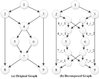

![table to guide the searching procedure of ants, which is infavor of addressing traditional path-finding problems such astravelling salesman problems [14], [20]](https://thumb-us.123doks.com/thumbv2/123dok_us/8683107.378599/12.612.52.290.600.730/searching-procedure-addressing-traditional-nding-problems-astravelling-salesman.webp)