Abstract—Routers typically provide a value of aggregate traffic forwarded from source to destination during fixed inter-vals, however there is no information as to how this value has evolved within the interval. This paper presents a model for the evolution of user-router bandwidth demand based on a first-order linear stochastic differential equation driven by random disturbances. Having obtained a predicted estimate of the aggregate value at the end of the interval, an adaptive PID controller is used to control the stochastic process towards this estimate. Matlab/Simulink simulations are presented in typical network node scenarios for validation of the above modeling approach.
Index Terms—Adaptive PID controller, network traffic modeling, router bandwidth, stochastic modeling.
I. INTRODUCTION
OUTERS periodically provide to network administra-tors an aggregate value of packets (in Gbits) that have been forwarded from source to destination. This is usually done at the end of fixed intervals (typically 5 or 15 minutes), starting from a low handshake (or self check, or staying alive) value. However, no information is provided as to how this value of the user-router bandwidth demand has evolved within this interval.
The evolution of this value is random due to user behav-ior. If a router with 5 Gbps capacity had its buffer size com-pletely full for the whole duration of a 5-minute interval, then the evolution of the aggregate value would have not been random but constant at a level of 1500 Gbits. In prac-tice, the router buffer is not completely full within the 5-minute interval, due to the random user behavior and band-width demand. Thus the final aggregate value is obviously less than the deterministic value of 1500 Gbits at the end of the interval [1]. Further note that routers are not set up to provide the aggregate packet count at shorter intervals, since this would severely compromise their performance.
The available aggregate value at the end of each interval can be used by administrators to obtain a trend in network traffic. However, some knowledge of the evolution of band-width demand within the 5-minute interval would be very
Manuscript received March 23, 2015; revised April 16, 2015. I. K. Giannopoulos is with the Department of Information and Commu-nication Systems Engineering, University of the Aegean, Samos 83200, Greece (e-mail: [email protected]).
A. P. Leros is with the Department of Automation, Technological Insti-tute of Chalkis, Evia, Greece (e-mail: [email protected]).
A. K. Leros is with the Department of Information and Communication Systems Engineering, University of the Aegean, Samos 83200, Greece (e-mail: [email protected]).
helpful in improving quality of service (QoS). Thus, there is a need to model the evolution of the process within this interval with a model that follows the random user behavior for router bandwidth demand, with the constraint of a low handshake data rate demand at the beginning of each inter-val. The problem of providing information to administrators within fixed intervals for QoS purposes has been addressed in [2-5]. In [2] a QoS-aware procedure for bandwidth provi-sioning is given to determine the lowest required bandwidth capacity level for a network link based on a given traffic load, assumed to be Gaussian. In [3], the available band-width on a link is estimated for QoS purposes based on a linear regression model using time series data of past passive sample measurements taken with the MRTG package [4], usually every 5-minute intervals.
This paper presents a first-order linear model driven by random disturbances and controlled with an adaptive PID (proportional-integral-derivative) controller to provide the evolution of the user-router bandwidth demand within an interval, given an estimate of the aggregate value at the end of the interval that can be provided by a predictor algorithm. The structure of this paper is as follows: next section pre-sents the linear first-order model and its parameters with an adaptive PID controller to control the evolution of router bandwidth demand, based on the random user behavior. Section 3 presents Matlab/Simulink simulations results to validate the PID controlled modeling approach. Finally, Section 4 presents conclusions and possible further work.
II. MODEL FOR THE EVOLUTION OF ROUTER BANDWIDTH DEMAND WITH A PID CONTROLLER
A. Deterministic Model
Our objective is to obtain a model for the evolution of the router bandwidth demand y(t) within an interval (0, T), based on our knowledge of y(t) at the endpoints of this inter-val. As a first approach, we use a first-order linear system with time constant τ. The input to this system depends on the user behavior and consists of two components:
– a deterministic part u(t) representing the mean, or trend of user demand;
– a stochastic part w(t) modeling random fluctuations around the trend.
Alternatively, u(t) can be thought of as a control input that has to drive the system within the interval T from zero initial conditions, i.e. y(0) 0, to some aggregate bandwidth de-mand y(T) = yd. In practice, an estimate of yd can be
provid-ed in advance by a prprovid-edictor algorithm, such as a Kalman Filter, based on past router bandwidth demand sample data.
A Model for the Evolution of Router Bandwidth
Demand Using an Adaptive PID Controller
Iordanis K. Giannopoulos, Apostolos P. Leros, and Asimakis K. Leros
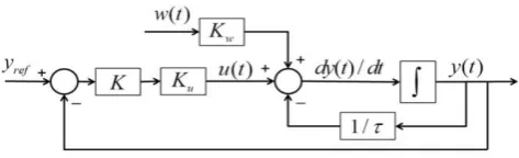
The evolution of the router bandwidth demand y(t) can be therefore described by the following open-loop system:
) ( ) ( ) ( ) / 1 (
/dt τ y t K ut K wt
dy u w . (1)
A block diagram of this system is given in Fig. 1.
At first suppose that the disturbance w(t) 0. The control objective then can be accomplished by applying a constant input u(t) U0. Assuming that T τ 300 sec, the
differen-tial equation (1) becomes:
0
/
(1 / 300) ( )
u;
(0)
0
dy dt
y t
K U
y
. (2)The solution to the initial value (2) then gives us the evo-lution of the router bandwidth demand within the 5-minute interval as follows:
/300 0
( )
300
u(1
t)
y t
K U
e
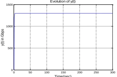
. (3)As an example, for a constant router capacity value of U0
5 Gbps, the maximum final output value is yd 300 U0
1500 Gbps, requiring a value of Ku 1 / (1 – e–1) 1.582.
Fig. 2 illustrates the evolution of y(t) in this case. For any final value less than the maximum output value, we solve (3) to obtain the relation Ku U0 0.0053 yd.
B. Stochastic Model
Now suppose that a disturbance bandwidth demand w(t) enters the system. Assuming a constant disturbance w(t) w0
0, the differential equation becomes:
0 ) 0 ( ; )
( ) / 1 (
/dt τ yt KU0 K w0 y
[image:2.595.311.536.53.228.2]dy u w . (4)
Fig. 1. Open-loop system modeling the evolution of bandwidth demand y(t).
0 50 100 150 200 250 300
0 500 1000 1500
Evolution of y(t)
Time(sec)
y(
t)
in
G
b
p
s
Fig. 2. Evolution of y(t) using the deterministic model with a constant user input u(t) = 5 Gbps
0 50 100 150 200 250 300
0 500 1000 1500 2000 2500 3000 3500
Time(sec)
y(
t)
i
n
G
b
p
s
[image:2.595.85.255.405.478.2]Evolution of y(t)
Fig. 3. Evolution of y(t) using the stochastic open-loop model with con-stant inputs u(t) = w(t) = 5 Gbps and calculated gain values Ku= 1.582,
Kw= 2.
The initial value problem (4) has the solution:
/
0 0
( )
(
u w)(1
t)
y t
K U
K w
e
. (5)This means that, at the end of the 300 sec interval, the re-lation Ku U0 0.0053 yd alone will overshoot a desired yd
value by an error of y(t) 300Kww0(1 e 1). As a result, the larger the disturbance is, the worse the relation Ku U0
0.0053 yd alone will do. This effect is illustrated in Fig. 3.
The above analysis indicates the problem with the open-loop control strategy. To remedy this situation, we consider the closed-loop control problem, with an input reference signal yref(t), as shown in Fig. 4.
The differential equation governing the closed-loop sys-tem is:
) ( ) ( )
( ) /
1 (
/dt τ K K y t K Ky t K wt
dy u u ref w . (6)
The evolution of the router bandwidth demand within the 5-minute interval, assuming a constant yref(t) yd and w(t)
w0 0, is given by the following solution of the closed-loop
system (6) to the initial value problem y(0) 0:
0
(1/ )
0 0
0
( )
(1
)
1 /
U K t
d w
U Ky
K w
y t
e
U K
. (7)An example of the evolution of y(t) in this case is pre-sented in Fig. 5. These results indicate that, although the response is fast, it also entails a significant error, deducing that the proportional gain controller K alone is not sufficient to reach the desired yd value.
[image:2.595.59.271.529.674.2] [image:2.595.309.546.640.712.2]0 50 100 150 200 250 300 0
500 1000 1500
Evolution of y(t)
Time(sec)
y(
t)
in
G
b
p
[image:3.595.305.549.49.169.2]s
Fig. 5. Evolution of y(t) using the closed-loop model with constant inputs u(t) = w(t) = 5 Gbps, and gain values Kw= 100, Ku= 0.5.
C. PID Controller
To remedy this situation a PID (proportional, integral, de-rivative) controller is proposed. The PID controller, operat-ing in the time domain, produces the control signal [5]
0
( )
( )
( )
( )
t
p i d
de t
u t
K e t
K
e
d
K
dt
, (8) where e(t) = y(t) – yref(t), and Kp, Ki, Kdare respectively theproportional, integral, derivative gains of the PID controller. We now consider the unknown disturbance bandwidth demand w(t) entering the system. In real world situations, the user bandwidth demand is random within the interval T. The instances that users appear within this interval are not known, neither are their bandwidth demands.
The random appearance of the users can be modeled by a Bernoulli distribution. Such a choice implements the actual behaviour of the user, which is of an on/off, or presence and absence, type. The Bernoulli probability distribution func-tion is given by [6]
otherwise 0
1 or 0 )
1 ( ) (
1 x
p p x f
x x
(9) The unknown bandwidth that a particular user will request is modeled by a uniform distribution. The uniform distribu-tion indicates equal probabilities among all possible values of bandwidth demand and is the most reasonable distribution in the absence of a priori statistical information about user behavior [6].
Based on the above discussion, our model of the random user input makes use of the following variables:
Bt: a Bernoulli random variable indicating the presence
or absence of a user request at time instant t [0, T]. Ut: a uniform random variable in [0, 1], representing the
relative amount of bandwidth that a user may request. Kw: a coefficient that sets the absolute limits of the above
uniform distribution.
The bandwidth that a random user will request at time in-stant t can therefore be described by the product Kw Bt Ut.
We further note that in practise Kw cannot exceed the desired
reference value yref adjusted by a low handshake data rate
value ylow of the router, which usually is around 4000bps, i.e.
Kw yref ylow.
[image:3.595.63.266.53.186.2]The above model for the random user appearance and the corresponding bandwidth demand can be used to represent
Fig. 6: Closed-loop system with PID controller for the evolution of band-width demand.
the disturbance to the first-order linear system (6) as:
( )
(
ref low)
t tw t
y
y
B U
. (10)Combining (8) and (10) we reach the block diagram for the closed-loop control problem (6) shown in Fig. 6. The differential equation governing the PID closed-loop system is:
0
1
(
) ( )
( )
(
)
(
)
t
p i d
p i ref ref low t t
dy
dy
K
y t
K
y
d
K
dt
T
dt
K
K t y
y
y
B U
(11)
In order to eliminate the integral sign in (11) we can dif-ferentiate (assuming constant disturbance) to get a second order closed-loop characteristic equation to determine the dynamics of the system. The evaluation of (11) at t 0 with y(0) 0, yref(0) 0, and w(0) 0 gives dy(0) / dt 0. Then
(11) may be solved explicitly or numerically.
With a router capacity rate U0 5 Gbps, we can choose in
(11) the PID controller gains to be adaptive functions of the desired input value yref and the router capacity rate, i.e.
Kp = yref / U0,
Ki = 0.0585 yref / U0, and
Kd = 0.01 yref / U0.
A Simulink [7] block diagram simulation of (11), in the Laplace domain, is given in Fig. 7.
III. SIMULATION RESULTS
Using the above Simulink model of eq. (11), we carried out three different simulation experiments demonstrating the evolutions of the bandwidth requested y(t) within a 5-minute interval, as follows:
Simulation 1: Minimal reference value yref 4000 bps.
Simulation 2: Reference value yref 1000 Gbps.
Simulation 3: Reference value yref 2000 Gbps.
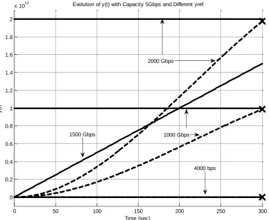
In all simulation experiments we have assumed a router capacity rate U0 5 Gbps. The results are shown in Fig. 8.
From the simulation results shown in Fig. 8 it is apparent that the PID closed-loop system (11) adequately models the stochastic evolution of the bandwidth demand y(t) for differ-ent reference values, including the random user behavior.
Note that in case the router had its buffer size completely full throughout the observation interval, then the bandwidth demand at every instant would be simply y(t) U0t, i.e. it
would increase linearly from zero to yref. Therefore the
dif-ference d(t) U0t y(t) can be used as an indicator of
Case 1: If, for some time instant t [0, T], d(t) 0, then the allocated bandwidth U0 is excessive.
Case 2: If, for some t, d(t) 0, then the allocated band-width U0 is sufficient.
Case 3: If, for some time instant t [0, T], d(t) 0, then the allocated bandwidth U0 is not sufficient.
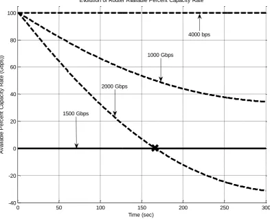
A plot of the percentile difference between y(t) and U0t
for the above three simulation experiments is shown in Fig. 9. As discussed above, such a plot can be used to indicate
[image:4.595.129.480.180.361.2]whether the available bandwidth is sufficient or not. From Fig. 9 it can be seen that, in the first two experiments, the available bandwidth is sufficient throughout the observation interval of 300 sec. In the third experiment, the available reaches zero at t = 160 sec, indicating that extra bandwidth is needed to accommodate the desired reference value.
Fig. 7: Implementation of the closed-loop system with adaptive PID controller using Simulink. The variables Bseed and Useed are the integer seeds used in the random number generator of the Bernoulli and uniform distributions, respectively.
0 50 100 150 200 250 300
0 0.2 0.4 0.6 0.8 1 1.2 1.4 1.6 1.8 2
x 1012 Evolution of y(t) with Capacity 5Gbps and Different yref
Time (sec)
y
(t
)
4000 bps 1500 Gbps
2000 Gbps
[image:4.595.110.503.407.728.2]1000 Gbps
Fig. 8: Results of three simulation experiments of the closed-loop system with adaptive PID controller within a 5-minute interval. Router capacity rate U0 = 5 Gbps in all cases. The observation interval is 300 sec. Experiment 1 (bottom): reference value is 4000 bps. Experiment 2 (middle): reference value is
0 50 100 150 200 250 300 -40
-20 0 20 40 60 80 100
Evolution of Router Available Percent Capacity Rate
Time (sec)
A
v
a
ila
b
le
P
e
rc
e
n
t
C
a
p
a
c
it
y
R
a
te
(
G
b
p
s
))
4000 bps
1000 Gbps
2000 Gbps
[image:5.595.106.500.55.374.2]1500 Gbps
Fig. 9: Percentile difference between the simulated bandwidth demand y(t) and a linearly increasing demand U0t. Experiment 1 (top): reference value is
4000 bps. The allocated bandwidth is excessive throughout the observation interval. Experiment 2 (middle): reference value is 1000 Gbps. The allocated bandwidth is sufficient throughout the observation interval. Experiment 3 (bottom): reference value is 2000 Gbps. The available bandwidth reaches zero at
t = 160 sec, indicating a lack of resources.
IV. CONCLUSIONS AND FURTHER WORK
This paper presented a linear first-order model with ran-dom disturbances describing the evolution of router capacity rate during a fixed interval, based on the knowledge (or prediction) of the corresponding values at the interval end-points. The model incorporates a PID controller with adap-tive gains based on the known parameters of the router. Simulation results were presented to validate that this model in fact gives an indication of the evolution of the router capacity rate. This model, and the corresponding evolution of bandwidth demand, can be used by network administra-tors to determine whether the available bandwidth is suffi-cient or not.
The value of bandwidth demand at the end of each fixed interval can be extrapolated from corresponding values at previous intervals. A predictor algorithm can be employed to estimate the bandwidth demand at the end of the current interval from previous values. The incorporation of a suita-ble predictor to the stochastic model presented herein is currently under investigation.
REFERENCES
[1] White Paper: Understanding fiber Ethernet bandwidth vs. end user experience [Online]. Available http://fiberinternetcenter .com/WhitePapers-Podcasts/WhitePaperEthervsEndUser.pdf
[2] H. van den Berg, M. Mandjes, R. van de Meent, A. Pras, F. Roijers, P. Venemans, “QoS-aware bandwidth provisioning for IP network links,” Computer Networks vol. 50, Aug. 2005, pp. 631–647. [3] T. Anjali, C. Scoglio, L. C. Chen, I. F. Akyildiz, G. Uhl, “ABEst: An
available bandwidth estimator within an autonomous system,” IEEE Global Telecommunications Conference, Nov. 2002.
[4] T. Oetiker, MRTG: Multi Router Traffic Grapher [Online]. Available:
http://people.ee.ethz.ch/oetiker/webtools/mrtg/
[5] D. Mahanta, M. Ahmed, U.J. Bora, “A study of Bandwidth Manage-ment in Computer Networks,” International Journal of Innovative Technology and Exploring Engineering, vol. 2, no. 2, Jan. 2013. [6] B. C. Kuo, F. Golnaraghi, Automatic Control Systems, John Wiley &
Sons, 2010.
[7] M. Evans, N. Hastings, B. Peacock, Statistical Distributions, John Wiley & Sons, 2000.
[8] Simulink manual [online]. Available: http://www.mathworks.com/