ISSN Online: 2327-4379 ISSN Print: 2327-4352
DOI: 10.4236/jamp.2018.66114 Jun. 28, 2018 1363 Journal of Applied Mathematics and Physics
Optimal Estimate of Quantum States
Mario Mastriani
Quantum Information Group, Merx Research, Aventura, FL, USA
Abstract
An optimal estimator of quantum states based on a modified Kalman’s filter is proposed in this work. Such estimator acts after a state measurement, allowing us to obtain an optimal estimate of the quantum state resulting in the output of any quantum algorithm. This method is much more accurate than other types of quantum measurements, such as, weak measurement, strong mea-surement, and quantum state tomography, among others.
Keywords
Kalman’s Filter, Quantum Algorithms, Quantum Measurement
1. Introduction
The problem of measurement in quantum mechanics [1] has been defined in various ways, originally by scientists, and more recently by philosophers of science who question the foundations of quantum mechanics. Measurements are described with diverse concepts in quantum physics such as:
wave-functions (probability amplitudes) which according to the linear Schrödinger equation involve a unitary and deterministic operator, thus pre-serving information,
superposition of states: linear combinations of wave-functions with complex coefficients that carry phase information and produce interference effects, known as the principle of superposition,
quantum jumps between states accompanied by the “collapse” of the wave-function that according to Dirac’s projection postulate in a von Neu-mann’s Process can destroy or create information,
collapses and jumps probabilities given by the square of the absolute value of the wave-function for a given state,
values for possible measurements given by the eigenvalues associated with the eigenstates of the combined measuring apparatus and measured system, in other words, the axiom of measurement,
How to cite this paper: Mastriani, M. (2018) Optimal Estimate of Quantum States. Journal of Applied Mathematics and Physics, 6, 1363-1381.
https://doi.org/10.4236/jamp.2018.66114
Received: May 24, 2018 Accepted: June 25, 2018 Published: June 28, 2018
Copyright © 2018 by author and Scientific Research Publishing Inc. This work is licensed under the Creative Commons Attribution International License (CC BY 4.0).
DOI: 10.4236/jamp.2018.66114 1364 Journal of Applied Mathematics and Physics the Heisenberg’s uncertainty principle.
The original problem stems from Niels Bohr’s “Copenhagen interpretation” of quantum mechanics since our measuring instruments, which are usually ma-croscopic objects and treatable with classical physics, can give us information about the microscopic world of atoms and subatomic particles like electrons and photons.
Bohr’s idea of “complementarity” insisted that a specific experiment could re-veal only partial information—for example, the position of the particle. Whereas “exhaustive” information requires complementary experiments, for example when determining the momentum of the particle, responding to the limits of the Heisenberg’s uncertainty principle.
Some of us define the problem of measurement simply as the logical contra-diction between two laws describing the motion of quantum systems: the first one talks about the unitary, continuous, and deterministic time evolution of the Schrödinger equation, whereas the second one involves their complete opposite counterpart, i.e., the non-unitary, discontinuous, and indeterministic collapse of the wave-function. John von Neumann saw a problem with two distinct (indeed, opposing) processes.
The mathematical formalism of quantum mechanics does not provide a way to predict when the wave-function stops evolving in a unitary fashion and col-lapses. Experimentally and practically, however, we can say that this occurs when the microscopic system interacts with a measuring apparatus.
Others define the measurement problem as the failure to observe macroscopic superpositions.
Decoherence theorists, e.g., H. Dieter Zeh and Wojciech Zurek, who use var-ious non-standard interpretations of quantum mechanics that deny the projec-tion postulate—quantum jumps—and even the existence of particles, define the measurement problem as the failure to observe superpositions such as Schrödinger’s cat. They also claim that unitary time evolution of the wave-function according to the Schrödinger wave-equation should produce such macroscopic superpositions.
Physics of Quantum Information treat a measuring apparatus in a quantum mechanically manner by describing its parts as in a metastable state like the ex-cited states of an atom: the critically poised electrical potential energy in the discharge tube of a Geiger counter, or the supersaturated water and alcohol mo-lecules of a Wilson cloud chamber. The pi-bond orbital rotation from cis- to trans- in the light-sensitive retinal molecule is an example of a critically poised apparatus.
magni-DOI: 10.4236/jamp.2018.66114 1365 Journal of Applied Mathematics and Physics tude more than the decrease in the small local entropy (an increase in stable in-formation or Shannon entropy) that constitutes the “measured” experimental data available to human observers.
The creation of new information in a measurement follows the same two core processes of all information creation—quantum cooperative phenomena and thermodynamics. These two are involved in the formation of microscopic ob-jects like atoms and molecules, as well as macroscopic obob-jects like galaxies, stars, and planets.
According to the correspondence principle, all the laws of quantum physics asymptotically approach the laws of classical physics in the limit of large quan-tum numbers and large numbers of particles. Thus, Quanquan-tum Mechanics can be used to describe large macroscopic systems.
Does this mean that the positions and momenta of macroscopic objects are uncertain? Yes, it does. Although the uncertainty becomes vanishingly small for large objects, it is not zero. Niels Bohr used the uncertainty of macroscopic ob-jects to defeat Albert Einstein’s several objections to quantum mechanics at the 1927 Solvay conferences.
But Bohr and Heisenberg also insisted that a measuring apparatus must be regarded as a purely classical system, since they cannot have it both ways: clas-sical and quantum. So, can the macroscopic apparatus also be treated by quan-tum physics or not? Can it be described by the Schrödinger equation? And, can it be regarded as in a superposition of states?
The most famous examples of macroscopic superposition are perhaps Schrödinger’s cat, which is claimed to be in a superposition of being alive and dead at the same time for a cat in a box, and the Einstein-Podolsky-Rosen expe-riment, in which entangled electrons or photons are in a superposition of two-particle states that collapse over macroscopic distances to exhibit properties “non-locally” at a speed faster-than-light.
These treatments of macroscopic systems with quantum mechanics were in-tended to expose inconsistencies and incompleteness in quantum theory. The critics hoped to restore determinism and “local reality” to Physics. They resulted in some strange and extremely popular “mysteries” about “quantum reality”, such as the “many-worlds” interpretation, “hidden variables”, and signaling at a faster-than-light speed.
Physics developed a quantum-mechanical treatment of macroscopic systems, especially a measuring apparatus to show how it can create new information. If the apparatus were describable only by classical deterministic laws, no new in-formation could come into existence. The apparatus needs to be adequately de-termined only, i.e., “classical” to a sufficient degree of accuracy.
Everything said so far indicates how sensitive is quantum computing to the correct measurement of the quantum states.
DOI: 10.4236/jamp.2018.66114 1366 Journal of Applied Mathematics and Physics In other words, none of the quantum measurement techniques currently in use: weak measurement, strong measurement, projective measurement and quantum state tomography allow a correct recovery of a generic quantum state resulting from the exit of a quantum algorithm without destructively distorting said state. This problem converts several (almost all) areas of Quantum Informa-tion Processing into mere theoretical speculaInforma-tions, namely: Quantum Algo-rithms, Quantum Image Processing, Quantum Signal Processing, Quantum Neural Networks, among others; which work fundamentally with generic qubits. Obviously, a new procedure to accurately estimate a generic quantum state is imperative as quantum technology advances.
Therefore, a new method of quantum measurement in the case of generic qu-bits becomes imperative (i.e., not just for CBS) and more accurate than the me-thods currently in use [4]-[26]. Thus, in this work, we present a novel proposal to recover quantum state to the output of a quantum algorithm after its mea-surement via a modified Kalman’s Filter [27] [28] [29] [30] [31], and Recursive Least Squares (RLS) filter [32] [33] [34], too. This is the essence of this work, which is organized as follows: Preliminaries to the new quantum measurement method are outlined in Section 2. A tour from Schrodinger equation to quantum algorithms is presented in Section 3. The new method (optimal state estimator) is outlined in Section 4. Finally, Section 5 provides a conclusion and future work proposals of this paper.
2. The Quantum Measurement Problem
In this section, we present the following topics: − Wave-function collapse.− Quantum Measurement Problem. − Before and after measurement.
− Types of measurement and state reconstruction.
2.1. Wave-Function Collapse
In quantum mechanics, wave-function collapse is the phenomenon in which a wave-function (initially in a superposition of several eigenstates) appears re-duced to a single eigenstate after interaction with a measuring apparatus [35]. It is the essence of measurement in quantum mechanics, and connects the wave-function with classical observables like position and momentum. Collapse is one of the two processes by which quantum systems evolve in time; the other is continuous evolution via the Schrödinger equation [36]. However in this role, collapse is merely a black box for thermodynamically irreversible interaction with a classical environment [37]. Calculations of quantum decoherence predicts apparent wave-function collapse when a superposition forms between the quan-tum system’s states and the environment’s states. Significantly, the combined wave-function of the system and environment continue to obey the Schrödinger equation [38].
post-DOI: 10.4236/jamp.2018.66114 1367 Journal of Applied Mathematics and Physics ulated that wave-function collapse cut the quantum world from the classical [39]. This tactical move allowed quantum theory to develop without distractions from interpretational worries. Nevertheless, it was debated if the collapse was a fundamental physical phenomenon, rather than just the epiphenomenon of some other processes. If this is the case, then, it would mean that nature is fun-damentally stochastic, i.e. nondeterministic, and an undesirable attribute for a theory [37] [40] [41]. This issue remained incomplete until quantum decohe-rence entered mainstream opinion after its reformulation in the 1980s [4] [37] [38]. Decoherence explains the perception of wave-function collapse in terms of interacting large- and small-scale quantum systems, and is commonly taught at the graduate level, e.g. the Cohen-Tannoudji textbook [42]. The quantum filter-ing approach [43] [44] [45] [46] and the introduction of quantum causality non-demolition principle [47] allows us to think about a classical-environment derivation of wave-function collapse from the stochastic Schrödinger equation.
2.2. The Quantum Measurement Problem Itself
The measurement problem in quantum mechanics is the unresolved problem of how (or if) wave-function collapse occurs. The inability to observe this process directly has given rise to different interpretations of quantum mechanics, and poses a key set of questions that each interpretation must answer. The wave-function in quantum mechanics evolves deterministically according to the Schrödinger equation as a linear superposition of different states, but actual measurements always find the physical system in a definite state. Any future evolution is based on the state the system was discovered to be in when the measurement was made, meaning that the measurement “did something” to the process under examination. Whatever that “something” done does not appear to be explained by the basic theory.
To express matters differently (according to Steven Weinberg [4] [5]), the Schrödinger wave-equation will determine the wave-function at any later time. If observers and their measuring apparatus are themselves described by a determi-nistic wave-function, why can we not predict precise results for measurements, but only probabilities? As a general question: how can one establish a corres-pondence between quantum and classical reality? [6].
2.3. Before and after Measuring
DOI: 10.4236/jamp.2018.66114 1368 Journal of Applied Mathematics and Physics general [48].
Postulate. Quantum measurements are described by a set of measurement operators
{ }
Mˆm , which are indexed with m labels for the different measure-ment outcomes. These outcomes act on the state space of the system being measured. Measurement outcomes correspond to values of observables, such as position, energy and momentum, which are Hermitian operators [48] [49] cor-responding to physically measurable quantities.Let ψ be the state of the quantum system immediately before the mea-surement. Then, the probability that the m-th results occurs by
( )
ˆ ˆ†m m
p m = ψ M M ψ (1) where ˆ†
m
M is the adjoint of Mˆm, and the post-measurement quantum state is
† ˆ
ˆ ˆ
m pm
m m
M M M
ψ
ψ
ψ
ψ
= (2)
Operators Mˆm must satisfy the completeness relation [48], i.e., †
ˆ ˆm m
mM M =I
∑
because it guarantees that probabilities will sum to one:
( )
†
ˆ ˆm m 1
m ψ M M ψ = mp m =
∑
∑
Let us work out a simple example, assuming we have a polarized photon with associated polarization orientations “horizontal” and “vertical”, where the hori-zontal polarization direction is denoted by
[
]
T0 = 1 0 , the vertical polariza-tion direcpolariza-tion is denoted by 1 =
[
0 1]
T, and (•)T is the transpose of (•). Thus, an arbitrary initial state for our photon can be described by the generic quantum state ψ =α 0 +β 1 , where α and
β
(α ≤1, β ≤1) are complexnum-bers constrained by the normalization condition 2 2
1
α + β = and
{
0 , 1}
is the computational basis spanning in the Hermitian space Η2.
Now, we construct two measurement operators Mˆ0= 0 0 and 1
ˆ 1 1
M = and two measurement outcomes a a0, 1. Then, the full observable used for measurement in this experiment is M aˆ = 0 0 0 +a1 1 1 . According to the Postulate, the probabilities of obtaining outcome a0 or outcome a1 are given by
( )
20
p a = α and
( )
2 1p a = β . Corresponding post-measurement quantum states are as follows: if outcome is equal to a0 then ψ pm= 0 ; if outcome is equal to a1 then, ψ pm= 1 .
2.4. Types of Measurement and State Reconstruction
As we have seen in the previous subsection, quantum measurement is not a mi-nor issue [4] [5] [6]. In fact, it is an issue still unresolved [7] [8], which would make it impossible for every practical effort to implement any genuine quantum algorithm in general and quantum image processing algorithm in particular. Actually, it is an inherited problem of quantum physics also known as the para-dox of measurement [9] [10] [11] [12].
DOI: 10.4236/jamp.2018.66114 1369 Journal of Applied Mathematics and Physics processing, the problem is reduced to the following: suppose we develop a quantum algorithm for filtering classic images. Clearly, the first problem would be, how to introduce a classical noisy image within a quantum computer, i.e., the design of the interfaces classical-to-quantum, and quantum-to-classical. But, the second would be, how to measure the results of a quantum filtering algorithm, and to take the result of that filtering process and carry it out to the classical world, in other words, the recovery of the classical version of the filtered image into its original space: the classical world where it was generated. It is obvious that an absolutely accurate technique of measurement is needed. Unfortunately, all efforts in this regard have been useless [13] [14].
However, in the last decade there have been several efforts to remedy this sit-uation, namely:
− Weak measurement
− Restoring the quantum state − Quantum state tomography
Weak measurement is a technique to measure the average value of a quan-tum observable ψ pm without appreciably affecting the initial state ψ of the system being measured [15] [16] [17] [18] [19]. Weak measurements differ from normal (sometimes called “strong” or “von Neumann”) measurements in two ways:
1) If ψ pm has discrete spectrum (which we assume for simplicity purposes), a strong measurement yields an eigenvalue of ψ pm when the system is in a
ψ state. If the measurement is repeated many times, starting each time with the system in a ψ state, one obtains a sequence of eigenvalues of ψ pm which when averaged yields an approximation to ψ ψpmψ , the expectation of ψ pm in the ψ state.
By contrast, a weak measurement only yields a sequence of numbers which average to ψ ψpmψ . For example, a strong measurement of the spin of a par-ticle with a spin −1/2 must yield spin 1/2 or −1/2, but a particular weak mea-surement could yield spin 100, while a subsequent weak meamea-surement on an identical system might be −128.3. Typically, a single weak measurement gives little information; only the average of a large number of such measurements is meaningful.
2) A strong measurement changes, or projects, an initial pure state ψ to an eigenvector of ψ pm. The particular eigenvector obtained cannot be predicted, though its probability is determined. This substantially changes the ψ state unless ψ happened to be close to that eigenvector.
However, a weak measurement does not substantially change the initial state. Weak measurements are usually implemented by coupling the original system
DOI: 10.4236/jamp.2018.66114 1370 Journal of Applied Mathematics and Physics States which are not product states are called entangled states.
The results obtained by this technique are as weak as its name, therefore, we proceed to the next.
Restoring the quantum state is an effort to recover the original ψ state from the alleged reversibility of a measurement operator through the matrix that represents such operator, that is to say,
M
ˆ
of Subsection 2.3 [20]. Parrott’s work is presented in opposition to the technique of weak measurement in gener-al and Katz etal. work [17] in particular. Other relevant works mediate between the above [21] [22], also without success.Nowadays, we know based on Stochastic Processes and Adaptive Filtering [27]-[34] that the single matrix inversion in an estimate or identification process does not restore the state of a hidden system behind such matrix. This is due to the need of modeling the state, the measurement noises, and defining the archi-tecture of the estimator in an accurate way for a correct system state recovery from the observables. This deficiency explains why Wiener’s filter was com-pletely replaced by Kalman’s filter in the presence of such noises [27] [28] [29] [30] [31]. Therefore, this technique is as weak as that to which it opposes.
Quantum state tomography is the process of reconstructing the quantum state (via a density matrix) for a source of quantum systems by measurements done on the systems coming from that source [33] [24]. Being the density matrix for pure or mixed states,
( )
ˆ mp m m m
ρ=
∑
ψ ψ (3)The source may be any device or system which prepares quantum states either consistently into quantum pure states or otherwise into general mixed states. To be able to uniquely identify the state, the measurements must be tomographical-ly complete. That is, the measured operators must form an operator basis on the Hilbert space of the system, providing all the information about that state. Such a set of observations is sometimes called a quorum. On the other hand, in a quantum process tomography, known quantum states are used to prove if such quantum process can find out how that process can be described. Similarly, quantum measurement tomography works to find out what measurement is be-ing performed. The general principle behind quantum state tomography is that by repeatedly performing many different measurements on quantum systems described by identical density matrices frequency counts can be used to infer probabilities. These probabilities are combined with Born’s rule to determine a density matrix which fits best with the observations [25] [26]. Obviously, this method is a rustic estimator of the density matrix and not the states themselves. In fact, it is a monitor of the elements of the matrix, only. Therefore, our prob-lem persists.
3. From Schrödinger’s Equation to Quantum Algorithms
3.1. Schrödinger’s Equation and the Unitary Operators
DOI: 10.4236/jamp.2018.66114 1371 Journal of Applied Mathematics and Physics symbolized as U, with U U I† = , where U† is the adjoint of U and I is the identity matrix, which is required to preserve the inner products: If we trans-form χ and ψ to U χ and U ψ , then χ U U† ψ = χ ψ , being
χ and ψ two wave-functions. In particular, unitary operators preserve lengths: ψ U U† ψ = ψ ψ =1.
On the other hand, the unitary operator satisfies the following differential eq-uation known as the Schrödinger’s eqeq-uation [49] [50] [51] [52]:
( )
ˆ( )
d d
iH
U t U t
t
− =
(4)
where ˆH represents the Hamiltonian matrix of the Schrödinger’s equation, 2 1
i= − , and
is the Planck constant. Multiplying both sides of Equation (4) by ψ( )
0 and setting ψ( )
t =U t( ) ( )
ψ 0 , yields( )
ˆ( )
d d
iH
t t
t ψ ψ
− =
(5)
The solution to the Schrödinger’s equation is given by the matrix exponential of the Hamiltonian matrix for the time invariant case:
( )
e iHtˆU t = − (6)
Thus, the probability amplitudes evolve across time according to the following equation:
( )
t e iHtˆ( )
0ψ = − ψ (7)
Equation (7) is the main piece in building circuits, gates and quantum algo-rithms, being U who represents such elements [49].
Finally, the discrete version of Equation (5) is
1 ˆ
t iH t
ψ
+ψ
− =
(8)
Equation (8) is the foundation on which we build the optimal estimator of quantum states.
3.2. Quantum Circuits, Gates and Algorithms
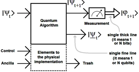
As we can see in Figure 1, and remember Equation (8), the quantum algorithm (with identical considerations for circuits and gates) can be seen as a transfer (that makes an input-to-output mapping) that has two types of output:
a) the result of the algorithm (circuit of the gate), i.e., ψt+1 , and
b) part of the input ψt , i.e., ψt (underlined ψt ), in order to impart reversibility to the circuit, which is a critical need in quantum computing [1].
DOI: 10.4236/jamp.2018.66114 1372 Journal of Applied Mathematics and Physics
Figure 1. Module to measuring, quantum algorithm and the elements needed to their physical implementation.
wire carrying 1 qubit or N qubits (qudit), interchangeably, while a single thick line represents a wire carrying 1 or N classical bits, interchangeably, too.
However, the mentioned concept of reversibility is closely related to energy consumption, and hence to the Landauer’s Principle.
On the other hand, computational complexity studies the amount of time and space required to solve a computational problem. Another important computa-tional resource is energy. In this section, we study the energy requirements for computation. Surprisingly, it turns out that computation, both classical and quantum, can in principle be done without expending any energy. Such energy consumption in computation turns out to be deeply linked to the reversibility of the computation.
What is the connection between energy consumption and irreversibility in computation? Landauer’s principle provides the connection, stating that, in or-der to erase information, it is necessary to dissipate energy. More precisely, Landauer’s principle may be stated as follows:
Landauer’sprinciple (firstform): Supposeacomputererasesasinglebitof information. The amountof energy dissipated intothe environmentis atleast kBTln 2, wherekBisauniversalconstantknownasBoltzmann’sconstant, andT
isthetemperatureoftheenvironmentaroundthecomputer.
According to the laws of thermodynamics, Landauer’s principle can be given an alternative form stated not in terms of energy dissipation, but rather in terms of entropy:
Landauer’sprinciple (secondform): Supposeacomputererasesasinglebit of information. The entropy of the environment increases by at least kB ln2,
wherekBisBoltzmann’sconstant.
under-DOI: 10.4236/jamp.2018.66114 1373 Journal of Applied Mathematics and Physics standing irreversibility is to think of it in terms of information erasure. If a logic gate is irreversible, then some of the information input to the gate is lost irre-trievably when the gate operates—that is, some of the information has been erased by the gate.
Conversely, in a reversible computation, no information is ever erased, be-cause the input can always be recovered from the output. Thus, saying that a computation is reversible is equivalent to saying that no information is erased during the computation.
Summing-up, the above expressed justifies the inexcusable need for the pres-ence of ψt to the output of the quantum gate [49].
4. Optimal State Estimator (OSE)
4.1. Classical State Estimator in Noiseless Environments
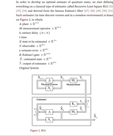
In order to develop an optimal estimate of quantum states, we start defining everything on a classical type of estimator called Recursive Least Square RLS [32] [33] [34] and derived from the famous Kalman’s filter [27] [28] [29] [30] [31]. Such estimator (in time discrete version and in a noiseless environment) is based on Figure 2, in which,
A: plant
∈
N N×
M: measurement operator
∈
M N×Δ: unitary delay
(
N N×)
t: time
X: state to be estimated
∈
N×1
Y: observable
∈
M×1ε: estimate error
∈
M×1
K: Kalman’s gain
∈
N M׈
X
: estimated state∈
N×1
ˆ
Y
: output of estimator∈
M×1 [image:11.595.152.537.274.738.2]OriginalSystem:
DOI: 10.4236/jamp.2018.66114 1374 Journal of Applied Mathematics and Physics
1
t t t
X =A X− (9)
t t t
Y M X= (10)
Estimator:
1
ˆt t ˆt t t
X =A X− +Kε (11) ˆt t ˆt
Y M X= (12) Then, we can define apriori and aposteriori (respectively) estimate error as:
ˆ ˆ
t Y Yt t Y M Xt t t
ε−= − −= − − (13)
and
ˆ ˆ
t Y Y Y M Xt t t t t
ε = − = − (14)
The apriori estimate error covariance is then
( )( )
{
T}
{
(
ˆ)(
ˆ)
T}
t t Y M Xt t t Y M Xt t t
ε− ε− − −
Ξ = Ξ − − (15)
where Ξ
{ }
• means square error of “•”, and (•)T means transpose of “(•)”. On the other hand, the aposteriori estimate error covariance is{ }
T{
(
ˆ)(
ˆ)
T}
t t Y M X Y M Xt t t t t t
ε ε
Ξ = Ξ − − (16)
This adaptation process is based on the minimization of the mean square er-ror criterion defined in the last equation. Developing Equation (16), rearranging terms, and minimizing the mean square error with respect to
X
ˆ
, we obtain the Wiener’s filter for stationary signals:1
ˆ MM MY
X R r= − (17) where, RMM is the autocorrelation matrix M and rMY is the cross-correlation
vector of M and Y. In the following equation, we formulate a recursive, time-update and adaptive version of Equation (17). In fact, RMM can be
ex-pressed in a recursive fashion as
T
, , 1
MM t MM t t t
R =R − +M M (18)
To introduce adaptability to the time variations of the signal statistics, the au-tocorrelation estimate in Equation (18) can be windowed by an exponentially decaying window:
T
, , 1
MM t MM t t t
R =λR − +M M (19)
where
λ
is the so-called adaptation, or forgetting factor, and is in the range0
< <
λ
1
. Similarly, the cross-correlation vector can be calculated in a recursive form as, , 1
MY t MY t t t
r =r − +M Y (20)
This equation can be made adaptive using an exponentially decaying forget-ting factor
λ
again:, , 1
MY t MY t t t
DOI: 10.4236/jamp.2018.66114 1375 Journal of Applied Mathematics and Physics For a recursive solution of the least square error Equation (21), we need to obtain a recursive time-update formula for the inverse matrix in the form
1 1
, , 1
MM t MM t t
R− R− Update
−
= + (22)
where “Updatet” is an updated factor to be actualized in each step of time. After an extensive series of considerations, developments and replacements, such as
1
, ,
MM t MM t
P =R− , we get the following set of equations related to RLS adaptation algorithm [32] [33] [34] in a very similar form to Kalman’s filter [27] [28] [29] [30] [31].
Initialvalues:
,0 MM
P =δI (23) being I the identity matrix and
δ
a number different to 00
ˆ ˆI
X =X (24)
Filtergainmatrix:
1 T
, 1 , 1
t MM t t t MM t t
K P− M λI M P− M −
− −
= + (25)
Errorsignalequation:
1
ˆ
t Y M Xt t t
ε− −
−
= − (26)
Estimatedstates:
1
ˆt ˆt t t
X X− Kε− −
= − (27)
Inversecorrelationmatrixupdate:
[
]
1
, , 1
MM t t t MM t
P λ− I K M P−
−
= − (28)
Discreteestimatortime-updateequations:
1
ˆt t ˆt
X− A X −
= (29)
T
, 1 , 1
MM t t MM t t
P− A P A
− = − (30)
Indeed, A and M are time-invariant [27]-[34]. However, Equation (30) should be modified to work in noiseless environments, which are the most real scena-rios the filter will be used.
4.2. Quantum State Estimator in Noiseless Environments
From Equation (2), we have† ˆ ˆ ˆ m pm m m M M M
ψ
ψ
ϕ
ψ
ψ
= = (31)
being ˆ ˆ† m m M M
ψ ψ a norm of Mˆm, as follows,
† ˆm ˆ ˆm m
M =
ψ
M Mψ
(32)In fact, we can take any norm of Mˆm, even for different ψ of the original.
DOI: 10.4236/jamp.2018.66114 1376 Journal of Applied Mathematics and Physics
ˆ
ˆm m
m
M M
M
ϕ = ψ = ψ (33)
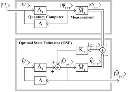
for each m, i.e., a battery of estimators as shown in Figure 3.
According to Figure 3, A will be the quantum algorithm (circuit or gate), and, we can get ψ for each m with this estimator. Therefore, the complete set of equations is:
InsideQuantumComputer: 1
t At t
ψ+ = ψ (quantum algorithm) (34)
1 1
t Mt t
ϕ+ = ψ + (quantum measurement) (35)
OptimalStateEstimator(OSE):
1 1
ˆt At ˆt Kt t
ψ+ = ψ + ε+ (36)
1 1
ˆt Mt ˆt
ϕ+ = ψ+ (37)
Estimateerror:
1 1 ˆ 1
t t t
ε+ = ϕ+ − ϕ+ (38) Three important considerations:
although A is time-invariant, this methodology also resists the variant ver-sion. In fact, we can do similar considerations relating to M. Besides, A arises
from Equation (7), i.e.,
ˆ e iHt
A U= = − , then:
( )
t e iHtˆ( )
0(
t t)
e iH tˆ( )
tψ
−ψ
ψ
− ∆ψ
= → + ∆ =
, which in its discrete
version will be:
(
ψt+1 =Ut t+1, ψt)
→(
ψt+1 =At ψt)
, OSE is a reorganized RLS/Kalman’s filter, but it is the same as them algo-rithmically speaking, and we started with a poor measurement, however as OSE evolves the accuracy of estimate improves through successive measure-ments.
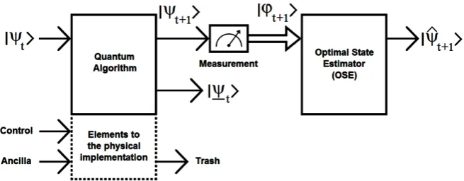
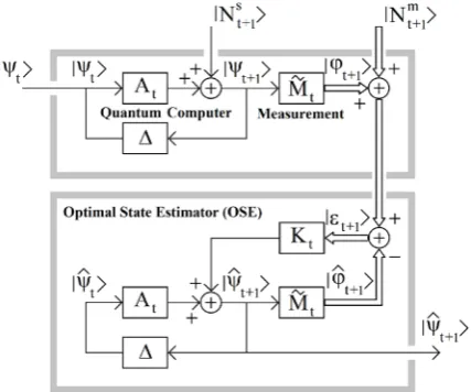
Figure 4 shows the complete schematic of Figure 1 but now with the OSE added to its output.
[image:14.595.261.486.539.701.2]DOI: 10.4236/jamp.2018.66114 1377 Journal of Applied Mathematics and Physics
Figure 4. Quantum algorithm (circuit or gate), measurement and OSE.
4.3. Quantum State Estimator in Noisy Environments
We assume the existence of state and measurement noises, as seen in Figure 5, with equation inside a quantum computer
1 s1
t At t Nt
ψ + = ψ + + (quantum algorithm) (39)
1 1 m1
t Mt t Nt
ϕ+ = ψ+ + + (quantum measurement) (40)
where, the random variables Nts+1 and Ntm+1 represent the state and measure-ment noises, respectively. Both are assumed to be independent of each other. In practice,
− the state noise covariance
{
( )( )
s s T}
t t
Q= Ξ N N , and
− the measurement noise covariance
{
( )( )
m m T}
t t
R= Ξ N N
matrices might change with each time-step or measurement, however here we assume that both are constant. Thus, only three equations change regarding classic estimator, namely,
Filtergainmatrix:
1 T
, 1 , 1
t MM t t t MM t t
K P− M R M P− M −
− −
= + (41)
Inversecorrelationmatrixupdate:
[
]
, , 1
MM t t t MM t
P I K M P−
−
= − (42)
Discreteestimatortimeupdateequation: T
, 1 , 1
MM t t MM t t
P− A P A Q
− = − + (43)
However, and as the OSE is a linear system, we can move the state noise to the output and work with a unique noise that represents both. Therefore, the last equation is not used.
All these noises may be associated with different factors: quantum noise [48] [49] [53] [54] [55], quantum decoherence [48] [56]-[61], and measurement er-rors [4]-[26]. The accuracy of our estimator (OSE) depends on two aspects our ability to model these noises, and
DOI: 10.4236/jamp.2018.66114 1378 Journal of Applied Mathematics and Physics
Figure 5. Modified Kalman’s estimator for noisy environments.
5. Conclusions and Future Works
In this paper, we have presented an optimal estimator of quantum states based on a modified Kalman’s Filter. Such estimator acts after state measurement, al-lowing us to obtain an optimal estimate of the quantum state resulting in the output of any quantum algorithm (circuit or gate). Finally, the OSE allows us a complete estimate of the quantum state in a much more accurate way than me-thods currently in use, which are: weak measurement, strong measurement, projective and quantum state tomography.
All of them fail to give an exact value for the state of a generic qubit resulting from a quantum algorithm. This lack can be seen explicitly in those algorithms involved in Quantum Image Processing (QImP) [62]. In that paper, it is clearly shown that quantum measurement itself acts as a noise that disturbs what is measured, e.g., if the quantum algorithm used consists of a filter which elimi-nates the noise of an image (inside quantum machine), the quantum measure-ment—on its way out—will add a new noise to the resulting image, i.e., the im-age returns to have noise. A question arises automatically: why do we then in-troduce the image into a quantum machine if after all the filtering must be done in the classical environment, that is, outside the quantum machine? For this reason, it is very important to apply the innovation of this paper to those algo-rithms used in QImP.
Finally and based on our current study, the solution presented in this paper for an optimal estimate of a generic quantum state is essential to effectively and efficiently face the simulation of all types of quantum algorithms involved in quantum information processing, in general, and quantum signal processing and quantum neural networks, in particular.
Acknowledgements
DOI: 10.4236/jamp.2018.66114 1379 Journal of Applied Mathematics and Physics
References
[1] Busch, P., Lahti, P., Pellonpää, J.P. and Ylinen, K. (2016) Quantum Measurement. Springer, New York. https://doi.org/10.1007/978-3-319-43389-9
[2] Mastriani, M. (2015) Quantum Boolean Image Denoising. QuantumInformation Processing, 14, 1647-1673. https://doi.org/10.1007/s11128-014-0881-0
[3] Mastriani, M. (2014) Quantum Edge Detection for Image Segmentation in Optical Environments. arXiv:1409.2918 [cs.CV]
[4] Weinberg, S. (1998) The Oxford History of the Twentieth Century. Howard, M. and Louis, W.R., Eds. Oxford University Press, Oxford, 26.
[5] Weinberg, S. (2005) Einstein’s Mistakes in Physics Today. PhysicsToday, 58, 31.
https://doi.org/10.1063/1.2155755
[6] Zurek, W.H. (2003) Decoherence, Einselection, and the Quantum Origins of the Classical. Reviews of Modern Physics, 75, 715-775.
https://doi.org/10.1103/RevModPhys.75.715
[7] Volz, J., etal. (2011) Measuring the Internal State of a Single Atom without Energy Exchange. arXiv:1106.1854v1 [quant-ph]
[8] Koashi, M. and Imoto, N. (2001) What Is Possible without Disturbing Partially Known Quantum States? arXiv:quant-ph/0101144
[9] Bohm, D. (1951) Quantum Theory. Prentice-Hall Inc., New York.
[10] Ghirardi, G.C., Rimini, A. and Weber, T. (1980) A General Argument against Su-perluminal Transmission through the Quantum Mechanical Measurement Process.
LettereAlNuovoCimento, 27, 293-298. https://doi.org/10.1007/BF02817189 [11] Merzbacher, E. (1970) Quantum Mechanics. John Wiley and Sons, New York. [12] Redhead, M. (1990) Incompleteness, Nonlocality, and Realism. Oxford University
Press, Oxford.
[13] Duty, T., et al. (2008) Observation of Quantum Capacitance in the Cooper-Pair Transistor. arXiv:cond-mat/0503531 [cond-mat.supr-con]
[14] Sillanpaa, M.A., etal. (2006) Direct Observation of Josephson Capacitance. arXiv:cond-mat/0504517 [cond-mat.mes-hall]
[15] Hosten, O. and Kwiat, P.G. (2006) Weak Measurements and Counterfactual Com-putation. arXiv:quant-ph/0612159
[16] Kastner, R.E. (2017) Demystifying Weak Measurements. arXiv:1702.04021v2 [quant-ph]
[17] Katz, N., etal. (2008) Reversal of the Weak Measurement of a Quantum State in a Superconducting Phase Qubit. Physical Review Letters, 101, Article ID: 200401.
https://doi.org/10.1103/PhysRevLett.101.200401
[18] Berry, M.V., Brunner, N., Popescu, S. and Shukla, P. (2011) Can Apparent Super-luminal Neutrino Speeds Be Explained as a Quantum Weak Measurement? Journal of Physics A: Mathematical and Theoretical, 44, Article ID: 492001.
https://doi.org/10.1088/1751-8113/44/49/492001
[19] Lundeen, J.S. (2006) Generalized Measurement and Post-Selection in Optical Quantum Information. PhD Thesis, University of Toronto, Toronto.
[20] Parrott, S. (2013) Essay on Restoring the Quantum State after a Measurement.
http://www.math.umb.edu/~sp/restore2.pdf
[21] Bruder, C. and Loss, D. (2008) Viewpoint: Undoing a Quantum Measurement.
DOI: 10.4236/jamp.2018.66114 1380 Journal of Applied Mathematics and Physics
[22] Cheong, Y.W. and Lee, S.-W. (2012) Balance between Information Gain and Rever-sibility in Weak Measurement.
[23] Balló, G. (2009) Master of Engineering in Information Technology Thesis: Quan-tum Process Tomography Using Optimization Methods. University of Pannonia, Pannonia.
[24] Niggebaum, A. (2011) Quantum State Tomography of the 6 Qubit Photonic Sym-metric Dicke State. Master Thesis, Ludwig Maximilians Universität München. [25] Blume-Kohout, R. (2006) Optimal, Reliable Estimation of Quantum States. [26] Altepeter, J.B., Jeffrey, E.R. and Kwiat, P.G. (2005) Photonic State Tomography
Re-view Article. Advances in Atomic, Molecular, and Optical Physics, 52, 105-159.
https://doi.org/10.1016/S1049-250X(05)52003-2
[27] Grewal, M.S. and Andrews, A.P. (2001) Kalman Filtering: Theory and Practice Us-ing MATLAB. 2nd Edition, John Wiley & Sons, New York.
[28] Sanchez, E.N., Alanís, A.Y. and Loukianov, A.G. (2008) Discrete-Time High Order Neural Control: Trained with Kalman Filtering. Springer-Verlag, Berlín.
https://doi.org/10.1007/978-3-540-78289-6
[29] Dini, D.H. and Mandic, D.P. (2012) Class of Widely Linear Complex Kalman Fil-ters. IEEETransactionsonNeuralNetworksandLearningSystems, 23, 775-786.
https://doi.org/10.1109/TNNLS.2012.2189893
[30] Haykin, S. (2001) Kalman Filtering and Neural Networks. John Wiley & Sons, New York. https://doi.org/10.1002/0471221546
[31] Brookner, E. (1998) Tracking and Kalman Filtering Made Easy. John Wiley & Sons, New York. https://doi.org/10.1002/0471224197
[32] Farhang-Boroujeny, B. (1998) Adaptive Filtering: Theory and Applications. John Wiley & Sons, New York.
[33] Haykin, S. (2002) Adaptive Filter Theory. 3rd Edition, Prentice-Hall, New York. [34] Diniz, P.S.R. (2008) Adaptive Filtering: Algorithms and Practical Implementation.
2nd Edition, Kluwer Academic Publishers, New York.
https://doi.org/10.1007/978-0-387-68606-6
[35] Griffiths, D.J. (2005) Introduction to Quantum Mechanics, 2e. Pearson Prentice Hall, New York, Upper Saddle River, 106-109.
[36] Von Neumann, J. (1932) Mathematische Grundlagen der Quantenmechanik. Springer, Berlin.
[37] Von Neumann, J. (1955) Mathematical Foundations of Quantum Mechanics. Prin-ceton University Press, New York.
[38] Schlosshauer, M. (2005) Decoherence, the Measurement Problem, and Interpreta-tions of Quantum Mechanics. Reviews of Modern Physics, 76, 1267-1305.
https://doi.org/10.1103/RevModPhys.76.1267
[39] Zurek, W.H. (2009) Quantum Darwinism. Nature Physics, 5, 181-188.
https://doi.org/10.1038/nphys1202
[40] Bohr, N. (1928) The Quantum Postulate and the Recent Development of Atomic Theory. Nature, 121, 580-590. https://doi.org/10.1038/121580a0
[41] Bombelli, L. (2010) Wave-Function Collapse in Quantum Mechanics. Topics in TheoreticalPhysics, 10-13.
http://www.phy.olemiss.edu/~luca/Topics/qm/collapse.html
DOI: 10.4236/jamp.2018.66114 1381 Journal of Applied Mathematics and Physics
[43] Cohen-Tannoudji, C. (2006) Quantum Mechanics. 2 Volumes, Wiley, New York, 22.
[44] Belavkin, V.P. (1979) Optimal Measurement and Control in Quantum Dynamical Systems. Technical Report, Copernicus University, Torun, 3-38.
[45] Belavkin, V.P. (1992) Quantum Stochastic Calculus and Quantum Nonlinear Fil-tering. JournalofMultivariateAnalysis, 42, 171-201.
https://doi.org/10.1016/0047-259X(92)90042-E
[46] Belavkin, V.P. (1999) Measurement, Filtering and Control in Quantum Open Dy-namical Systems. Reports on Mathematical Physics, 43, A405-A425.
https://doi.org/10.1016/S0034-4877(00)86386-7
[47] Belavkin, V.P. (1994) Nondemolition Principle of Quantum Measurement Theory.
FoundationsofPhysics, 24, 685-714. https://doi.org/10.1007/BF02054669
[48] Venegas-Andraca, S.E. (2006) Discrete Quantum Walks and Quantum Image Processing. Centre for Quantum Computation, University of Oxford, Oxford. [49] Nielsen, M.A. and Chuang, I.L. (2004) Quantum Computation and Quantum
In-formation. Cambridge University Press, Cambridge.
[50] Kaye, P., Laflamme, R. and Mosca, M. (2004) An Introduction to Quantum Com-puting. Oxford University Press, Oxford.
[51] Stolze, J. and Suter, D. (2007) Quantum Computing: A Short Course from Theory to Experiment. WILEY-VCH Verlag GmbH & Co. KGaA, Weinheim.
[52] Busemeyer, J.R., Wang, Z. and Townsend, J.T. (2006) Quantum Dynamics of Hu-man Decision-Making. JournalofMathematicalPsychology, 50, 220-241.
https://doi.org/10.1016/j.jmp.2006.01.003
[53] Master, C.P. (2005) Quantum Computing under Real-World Constraints: Efficiency of an Ensemble Quantum Algorithm and Fighting Decoherence by Gate Design. PhD Thesis. Stanford University, Stanford.
[54] Arias, A., Gheondea, A. and Gudder, S. (2002) Fixed Points of Quantum Opera-tions. Journal of Mathematical Physics, 43, 5872-5881.
https://doi.org/10.1063/1.1519669
[55] Michalski, M. (2013) Computational Complexity in the Analysis of Quantum Oper-ations. In: Jamiolkowski, A., Ed., Open Systems, Entanglement and Quantum Op-tics, InTechOpen, London, 41-63.
[56] Alagic, G. and Russell, A. (2005) Decoherence in Quantum Walk on the Hypercube. [57] Dass, T. (2005) Measurements and Decoherence.
[58] Kendon, V. and Tregenna, B. (2002) Decoherence in a Quantum Walk on the Line. [59] Kendon, V. and Tregenna, B. (2003) Decoherence Can Be Useful in Quantum
Walks. Physical Review A, 67, Article ID: 042315.
https://doi.org/10.1103/PhysRevA.67.042315
[60] Kendon, V. and Tregenna, B. (2003) Decoherence in Discrete Quantum Walks. Se-lected Lectures from DICE 2002. LectureNotesinPhysics, 633, 253-267.
https://doi.org/10.1007/978-3-540-40968-7_18
[61] Romanelli, A., etal. (2005) Decoherence in the Quantum Walk on the Line. Journal of Physics A, 347c, 137-152. https://doi.org/10.1016/j.physa.2004.08.070