Study of the Interactions between Particles Based in Paraquantum Logic

http://dx.doi.org/10.4236/jmp.2012.35051 Published Online May 2012 (http://www.SciRP.org/journal/jmp)

Study of the Interactions between Particles Based in

Paraquantum Logic

João Inácio Da Silva Filho1,2

1_{Group of Applied Paraconsistent Logic, Santa Cecília University, Santos, Brazil} 2_{Institute for Advanced Studies, University of São Paulo, São Paulo, Brazil}

Email: inacio@unisanta.br

Received January 25,2012; revised February 10, 2012; accepted March 13, 2012

ABSTRACT

Paraquantum Logic (PQL) has its origins in the fundamental concepts of the Paraconsistent Annotated Logic (PAL) whose main feature is to be capable of treating contradictory information. In this work we presented a study of applica-tion of the PQL in resolution of phenomena of physical systems that involves the interactions between physical bodies or particles. Initially is considered that each particle or physical body that is in the physical world has a representative Lat-tice in the Paraquantum world. From this consideration is made a study of the phenomena of Paraquantum Entangle-ment modeling the interaction between particles based in fundaEntangle-mental concepts of the Paraquantum Logic. The mathe-matical relationships of representative Lattices of the Paraquantum Logic originate models with values that are identi-fied with some physical constants. In this work these paraquantum values are identiidenti-fied with the Universal constant of Gravity, proposed by Newton, and the constant K, that relates the Interaction Force in charged particles in the Cou-lomb’s Law. The results showed that the Paraquantum Logical Model elaborated starting from the fundamental con-cepts of the Paraquantum Logic (PQL) is adequate to support theories based in a Paraquantum Universe built by an infi-nite amount of Lattices and forming a Paraquantum net of infiinfi-nite dimensions.

Keywords: Paraconsistent Logic; Paraquantum Logic; Classical Physic; Relativity Theory; Quantum Mechanics

1. Introduction

The researches developed in Physical science have the main objective to find models capable to simulate with precision our reality. However, in many cases, the ex-pected results are not reached because the extracted sig-nals of information of the real world are incomplete and contradictory.

When we worked with the Classic Physics, the uncer-tainties, the ambiguities and inconsistencies in the ex-tracted information of the real world cause great difficul-ties for the creation of efficient models to simulate phe-nomena of real physical systems. Because of these prob-lems many researches are being developed to find mod-els based on non-Classic Logics. A Paraconsistent Logic (PL) is a non-classical logic which revokes the principle of non-Contradiction and admits the treatment of contra-dictory information in its theoretical structure [1-4]. The real applications of the PL in programming of computa-tion systems began with an interpretative form that it used annotations, and, for that reason, the PL passed to be denominated of Paraconsistent Annotated Logic (PAL).

The Paraconsistent Annotated Logics with annotation of two values (PAL2v) [3,4] is a class of Paraconsistent

Logics particularly represented through a Lattice of four vertices and from its foundations the Paraquantum Lo- gics PQL was created [5].

According to [5] we can obtain through the PAL2v a representation of how the annotations or evidences ex-press the knowledge about a certain proposition P. Con-sidering that μ is the Favorable Degree of evidence and λ is Unfavorable Degree of evidence, then the symbol P(μ, λ) can be read in the following way:

Let be P(, ) a Paraconsistent Logical Signal (see [4,5]) where the annotation is composed by favorable degree of evidence μand by unfavorable degree of evidence  and assigned to a proposition P. The logical negation of P is defined as: P_{ , } P_{ , }

PT = P(1, 1) → intuitive reading that P is inconsistent.

 

Pt = P(1, 0) → intuitive reading that P is true.

PF = P(0, 1) →intuitive reading that P is false.

P= P(0, 0) → intuitive reading that P is Indeterminate. In the internal point of the lattice which is equidistant from all four vertices, we have the following interpreta- tion: PI = P(0.5, 0.5) → intuitive reading that P is unde- fined.

sian Plane (USCP) we can get linear transformations for a Lattice k of analogous values to the associated Lattice τ of the PAL2v [5]. We obtain the following final trans-formation:



,



T X Y 



xy x y,  1



C

D

(1) According to the language of the PAL2v we have:

x = μ→ is the Favorable evidence Degree

y = λ→ is the Unfavorable evidence Degree.

The first coordinate of the transformation (1) is called

Certainty Degree DC. So, the Certainty Degree is ob-

tained by:

 

 

+ 1

ct

(2) The second coordinate of the transformation (1) is called Contradiction Degree Dct. So, the Contradiction Degree is obtained by:

D  

 

(3) The second coordinate is a real number in the closed interval [–1,+1]. The y-axis is called “axis of the contra-diction degrees”.

Since the linear transformation T(X,Y)shown in (1) is

expressed with evidence Degrees μ andλ, then from (2), (3) and (1) we can represent a Paraconsistent logical state

τ into Lattice τ of the PAL2v [5,6], such that:





μ,λ , + 1



      

 , 



D DC, ct



  

 

(4)

or

(5) where:

τ is the Paraconsistent logical state.

DC is the Certainty Degree obtained from the evidence Degrees μ and λ.

[image:2.595.109.490.364.722.2]

Dct is the Contradiction Degree obtained from the evi-dence Degrees μ and λ.

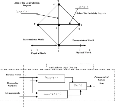
Figure 1 shows the Lattice of the LPA2v and where is obtained a point (DC, Dct) where DC = ƒ(μ,λ) and Dct = ƒ(μ,λ) which represents a Paraconsistent logical state ετ.

The main concepts and foundations of the logic LPA2v can be found in [5] and in [6]. Through the resul- tant equations of analyses in the PAL2v Lattice the prin- ciples of the Paraquantum Logic was created. This paper is organized in the following way: Section 2 shows the

Axis of the Certainty Degrees DC =  - λ

Axis of the Contradiction Degrees

Dct =  + λ - 1

T

+1

-1 

0

t F

+1 -1 0

Paraconsistent Logic(PAL2v)

λ μ

Observable Variables

Measurements Physical world

DC(μ, λ) = μ – λ

Dct(μ, λ) = μ + λ – 1

(D , D ) C ct

Paraconsistent Logical

State

Paraconsistent World _{Paraconsistent World}

1 μ Physical World

λ 1

Physical World

ετ

main concepts of the Paraquantum Logic, Section 3 a Paraquantum Logical model for quantization of values is proposed. In the Section 4 the phenomenon of Paraquan-tum Logical Entanglement and the effects of interactions among particles are studied with details and finally, the conclusion is presented in Section 5.

2. The Paraquantum Logic

P

QL

Under certain conditions the results obtained from the LPA2v model changed through leaps or unexpected va- riations [7]. This behavior in the resulting values demon- strates that the application of its foundations offered re- sults strongly connected to the ones found in modeling of phenomena studied in quantum mechanics (see [7,8]). Following this reasoning line a Paraquantum logical state

ψ is created on the lattice of the PQL as the tuple formed by the certainty degree DC and the contradiction degree

Dct [9,10]. Both values depend on the measurements per- fomed on the Observable Variables in the physical envi- ronment which are represented by μ andλ [10,11]. This way, we can express (2) and (3) in terms of μ and λ ob-taining:

( , ) C 

D   

) + 1

(6)

( , ct

D _{ }  



DC( , )  , Dct ( , ) 





DC( , )  , Dct ( , ) 





(1,1)



 

= t = 0,1



t





0, 1









1, 0



 



t (1,0)





1, 0



  

(7)

And a Paraquantum function (P) is defined as the Paraquantum logical state :

( )

ψ_PQ  (8)

For each measurement performed in the physical world of μ and λ, we obtain a unique duple

which represents a unique Paraquantum logical state ψ

which is a point of the lattice of the PQL[10]. On the ver- tical axis of contradictory degrees, the two extreme real Paraquantum logical states are:

1) The contradictory extreme Paraquantum logical state which represents InconsistencyT:

ψT DC(1,1), Dc

2) The contradictory extreme Paraquantum logical state which represents Undetermination:

ψ = =DC(0,0), Dc (0,0)

On the horizontal axis of certainty degrees, the two ex- treme real Paraquantum logical states are:

3) The real extreme Paraquantum logical state which represents Veracityt: ψt (1,0) t (1,0)

4) The real extreme Paraquantum logical state which

represents FalsityF: ψF .

,

C c

D D

D_C(1,0), D_c

A Vector of State P(ψ) will have origin in one of the two vertexes that compose the horizontal axis of the cer- tainty degrees and its extremity will be in the point formed for the pair indicated by the Paraquantum func-

tion (P) [10].

If the Certainty Degree is negative (DC < 0), then the Vector of State P(ψ) will be on the lattice vertex which is the extreme Paraquantum logical state False: ψF = (–1, 0).

If the Certainty Degree is positive (DC > 0), then the Vector of State P(ψ) will be on the lattice vertex which is the extreme Paraquantum logical state True: ψt = (1, 0).

If the certainty degree is nil (DC = 0), then there is an undefined Paraquantum logical state ψI =(0.0, 0.0).

The Vector of State P(ψ) will always be the vector ad-dition of its two component vectors:

C

X Vector with same direction as the axis of the cer-tainty degrees (horizontal) whose module is the comple- ment of the intensity of the certainty degree:

XC  1 DC

Y

Y D

ct Vector with same direction as the axis of the con-tradiction degrees (vertical) whose module is the contra-diction degree: ct  ct

Given a current Paraquantum logical state ψcur defined by the duple



DC( , ) , Dct( , ) 



then we compute the module of a Vector of State P(ψ) as follows:





2 ₂

(ψ) 1 C ct

MP   D  D

 

ψ 1 ψ

C R

D  MP

(9) where:

DC = Certainty Degree computed by (6)

Dct= Contradiction Degree computed by (7).

The real Certainty Degree (DCψR) is the value of the certainty degree without the effect of the contradiction. Using (9) which is for computing the module of a Vector of State P(ψ), we have:

1) For DC> 0 the real Certainty Degree is computed by: (10)

Therefore:





2 ₂

ψ 1 1

C R C ct

D    D D

ψ (ψ) 1

C R

D MP

(11)

2) For DC < 0, the real Certainty Degree is computed by:

(12)

 

Therefore:





2 ₂

ψ 1 1

C R C ct

D   D D 

ψ 0

C R

D 

(13)

where:

DCψR = real Certainty Degree.

DC= Certainty Degree computed by (6).

Dct= Contradiction Degree computed by (7). 3) For DC = 0, then the real Certainty Degree is nil:

ψ ψ 1 2 C R R D  

 (14)

The inclination angle  of the Vector of State is computed by:





ψ arctg

 1 ct C D D        

  (15)

2.1. Uncertainty Paraquantum Region

The propagation of the superposed Paraquantum logical states sup through the lattice of the PQL happens due to the continuous measurements performed on the Observ- able Variables in the physical world [10,11]. Since the Paraquantum analysis deals with favorable and unfavor- able evidence degrees μ and  of the measurements per- formed on the physical world, these variations affect the behavior and propagation of the superposed Paraquantum logical states sup on the lattice of the PQL.

When the module of the Vector of State MP(ψ) = 1, this vector will represent the maximal fundamental su- perposed Paraquantum logical states ψsupfmax which has real certainty degrees zero. The maximum Contradiction Degree for this condition is when the Vector of State P(ψ) forms an angle of 45˚ with the horizontal axis of cer- tainty degrees.

When the module of the Vector of State is of larger value than the unit MP(ψ) > 1, means that the Paraquan-tum logical state ψ are in an uncertainty region. The Pa- raquantum logical states into limits of the Region of Un- certainty are identified with Factors of maximum limita- tion of transition [10]. These factors are:

1) The factor of Paraquantum limitation False/incon- sistent—hQFT.

( )

1 2

ψ_PQ = 1

    _     

 ; 1 1; 1

2

1 _, 1

2   2 

    _{ }      

hQFT

2) The factor of Paraquantum limitation True/incon- sistent—hQtT.

( )

1 1;

2

ψ_PQ = 1

          _{ }

  1

1; 2

1 _, 1

2 2 

          

hQtT

3) The factor of Paraquantum limitation False/undeter- mined—hQF.

( )

0;

1-1 1

ψPQ = 1 _{ },

             _{ }     

 2 12 2 0; 1-12

                    _ 

mined—hQt.

hQF

4) The factor of Paraquantum limitation True/undeter-

( )

1 1

1 ;0 1 ; 0

2 2

1 1

ψ = 1 ,

2 2

PQ _{     }

                      _{ }      _{   }     

hQt

The unbalanced contradictory Paraquantum logical state

ψc

aquantum Factor of Quantization hψ 

tru is the one located on the lattice of states of the PQL where there is a condition of opposite signs between the Certainty Degree (DC) and the real Certainty Degree (DCψR).

2.2. The Par

When the superposed Paraquantum logical state sup propagates on the lattice of the PQL a value of quantiza-tion for each equilibrium point is established. This point is the value of the contradiction degree of the Paraquan-tum logical state of quantization h [10] such that:

ψ 2 1

h   (16) where: h is the Paraquantum Fact

ugh

aquantum logical state

ψ ψleap

h h

or of quantization. The factor h quantifies the levels of energy thro the equilibrium points where the Paraquantum logical state of quantization h, defined by the limits of propa-gation throughout the uncertainty of the PQL, is located.

Figure 2(a) shows the Paraquantum Factor of quanti-zation (h) and the interconnections between the factors and its characteristics, in which they delimit the Region of Uncertainty in the Lattice of PQL.

2.3. The Paraquantum Leap In a process of propagation of Par

, we have that in the instant that the superposed Paraq-uantum logical state sup reaches the representative points of the limiting factors of the uncertainty region of the PQL, the Certainty Degree (DC) remains zero but the real Certainty Degree (DCR)will be increased or de-creased from zero and this difference corresponds to the effect called of the Paraquantum Leap [10,11]. In order to completely express it, we have to take into account the factor related to the Paraquantum Leaps which will be added to or subtracted from the Paraquantum Factor of quantization[10] such that:

ψt

h   (17)

where, from Figure 2 we can make the calculations:



₁ 2 ₁



hψLeap hψ  (18)

So, the Factor of Paraquantum Qu co

antization in its mplete or total form which acts on the quantities is:



₁ 2 ₁



h_ψt h_ψ h_ψ  (19)

Being:



2



ψt 1 ψ 1

[image:4.595.318.536.85.130.2]

raquantum Quantization at the time of arrival of the Su-perposed Paraquantum Logical state ψsup at the point where the Paraquantum Logical state of Quantization ψhψ

is located.



2



ψ 1hψ 1 is the total Paraquantum Fac-

tor of Quantization at th

2.4. Newton Gamma Factor

its (SI), to express the

ψt

h h 

e departure of the Superposed Paraquantum Logical state ψsup at the point where the Paraquantum Logical state of Quantization ψhψ is located.

Figure 2(b) shows the effect of the Paraquantum Leap in the quantization of values when the Superposed Paraq-uantum Logical states sup reach the point where is the Paraquantum Logical state of Quantization ψhψ on the

PQL Lattice.

In the International System of un

value of force F in a unit of Newton, an adjustment on the value of mass is necessary [12]. Doing such comparisons and analogies between the International unit Systems (SI) and the British System we obtain for the proportionality factor k in the equation which expresses Newton’s sec-ond law (see [11,12]):

1.38254952

br

k   2 in the British System.

1 _{in the International} 0.723

IS

k  3013951

2

 System

of units (SI).

portance e Factor kbr,which will be

la , it

Given the im of th

rgely used in the equations of the PQL s value is called Newton Gamma Factor whose symbol is N [11].

Therefore, in order to apply classical logics in the Paraquantum Logical model, the Newton Gamma Factor is N  2.

2.5. Paraquantum Gamma Factor γPψ

The Lorentz Factor  can be identified in the infinite n

Power Series of the bi omial expansion [13,14] related to the series obtained from consecutively applying the Newton Gamma Factor N (see [11]).In the paraquan-tum analysis [10,11] we ine a correlation value called Paraquantum Gamma Factor ψ

def P

 such that:

ψ

P 1

N



 



   (20)

where:

N

 is the Newton Gamma Factor: _N  2

 is the Lorentz factor which is:

2

1

1 v

c



    _{ } Using the Paraquantum Ga Factor _ψ



mma _P allows

th

3. Paraquantum Logical Model Applied in

Th the PQL Lattice defines a

e computations, which correlate values of Observable Variables to the values related to quantization through

the Paraquantum Factor of quantization hψ[10,11].

Calculations of Quantization of Values of

Physical Quantities

e quantitative analysis on

quantitative value QValor of any physical quantity, which can be represented on the horizontal axis of the certainty Degrees and on the vertical axis of the contradiction de- grees of the PQL Lattice. Since the maximum value is normalized on the PQL Fundamental Lattice [10,11], con- sidering the Paraquantum factor of quantization only, we can write: 1hψ 



1 hψ



.

Doing so, in the PQL Fu amental Lattice the unitary nd va

ValuemaxFund ψ ValuemaxFund ψ ValuemaxFund where: QValuemaxFund is the value of the total amount

on the uni

tion (21) shows that the maximum amount of any qu

lue of the quantization is equivalent to a paraquantum quantization represented in the Paraquantum Logical state ψhψ added to the value of its complement. We have:



1



Q h Q  h Q (21)

rep-resented tary axis of the PQL Fundamental Lat-tice.

Equa

antity in the physical environment is composed by two quantized fractions where: one is determined on the Para- quantum Logical state of Quantization ψhψ by the Paraq-

uantum Factor of quantization hψ and the other is deter-

mined by its complement (1 – hψ). When the Paraquan-

tum Gamma Factor Pψ is applied on the paraquantum

quantities, besides co ating the paraquantum values to the physical environment, it also works as a factor of expansion or contraction of the PQL Lattice.

rrel

Representation of Levels of Energy in the

the involved Energy in the

Paraconsis-Totaψ ψ max Fund ψ maxFund (22) When related to the physical environment, we have: Lattice of PQL

By representing

tent Logical Model as being the energy amount repre-sented on the vertical axis of contradiction, we can ini-tially make an analogy with Equation (21) which defines the amount on the PQL Fundamental Lattice in its static form. So, for the Energy, the equation is:



1



E h E  h E





Physical Totaψ ψ

Physical ψ maxFund ψ maxFund

ψ ψ

1 1 ₁

P

P P

E E

E h E h E



 



  

(23)

The value of the quantity of Energy of Propagation qu

1



Paraquantum world Paraquantum world

Contradiction Degree

 

MP ψ 1

P()V =0°

D = hQt _{C = h}

Qt

1

2 2 h 





1h 1 2 1

P()t

 

MP ψ 1

Paraquantum Factor of Quantization

2 1 h 



P()F MP ψ 1

 

MP ψ 1

P()t = 45°

h

h

B = hQtT

IP

 

MP ψ 1 P()F

1 1 2  A=hQFT





1h 1 2 1

Paraquantum Factor of Quantization

2 1 h 

-1

Certainty Degree

DC

F



T

+1

t

-1

+1

1

2

1

2 2 h 

1

1 1 2 

1

2

1

DCψR

-DCψR

Paraquantum Leap

Physical world

Measurements Observable variable B

Physical world

Measurements Observable variable A

0

(a)

Paraquantum world Paraquantum world

Dct Contradiction

Degree

h

2 CψR ψ

D  1h 1

1

2 2 h



P()



h

IP   2 2

MP  1 Dct

1 1 2 

-1

Certainty DegreeDC



T

+1

t

-1

+1

1

2

1

2 2 h



1



1 1 2 

1

2

1

2

ψ

1 1

leap

h  h 

0

Physical world Measurements Observable Variable B

Physical world

Measurements Observable Variable A

(b)

[image:6.595.111.474.81.690.2]

is computed by:

ψ max N

P ropag N

E h E (24)

where:hψ is the Paraquantum Factor of quantization.

Propag

E is the Energy transformed in the propaga of t e Pa

tion h raquantum Logical state of the extreme Vertex False until it reaches the point where the Paraquantum Logical state of Quantization ψhψis located.

maxN

E is the maximum Energy on the level N of the transition frequency.

Since the process of transformation of energy is dyna- mical, we must consider the effects of Paraquantum Leaps on the Paraquantum Logical Model. So, the total energy transformed, that will constitute the Superposed Fundamental Lattice, will be obtained with adding the Inertial or Irradiating Energy Eirr that appears due to the effects of Paraquantum Leaps. Being the Factor of Quan-tization on the Paraquantum Leap defined on Equations (17) and (18), the Inertial or Irradiating Energy is ex- pressed by:



2





ψ

1h 1 (25)

So, the total energy transformed at th po

(26)



irrN maxN

E  E

e equilibrium int of the Lattice of the PQL is computed by:

transfTotalN PropagN irrN

E E E

or:



2





ψ

1 1

N h  (27)

So, Equation (22) is rewritten as follows:



transfTotalN maxN max

E h E E





TotalPropag transfTotal 1 ψ maxN

E E  h E (28)



1 ψ



max

or as follows:



Propag irr



TotalPropag N

E  E E

Or, in a more complete way, as fo

h E

  (29)

llows:







2

TotalPropag 1

E  h E E h











ψ max max ψ

ψ max

1

1

N N

N

h E



 

(30)

From Equation (23)









Propag irr

ψ max

1 _N

E E

h E 



 

 

(31)

The second term of Equations (30), (31) is the com- pl

Lattice of the PQL.

,

wh is is

After a paraquantum analysis, where the measurements en-

viron nce Degrees μ and λ

re are logically negated propositions. This TotalPropagPhysical

ψ

ψ

1

1

P

P

E

emented value which represents the remaining maxi- mum energy, therefore, it is that amount of energy capa- ble of still being transformed. So, the remaining energy

ERestmax is the one which outcomes the value which will be represented on the vertical and horizontal axis of the

4. The Paraquantum Logical Entanglement

and the Interaction between Particles

The phenomenon of Paraquantum Logical Entanglement is inherent to the foundations of Paraquantum Logics

ere the PAL2v is originated and where the analys only possible using two representing values of informa-tion (see [5]). Therefore, for the paraquantum analysis there will always be an entanglement of information from evidences about the proposition to be analyzed.

Considering the formalism of a Paraconsistent logic of two values (PAL2v) [4-6], the concept of Paraquantum logical state ψ on a system in a given instant can only be represented by the Paraquantum logical entanglement of the two Evidence Degrees λ and μ, which are obtained from measurements of the Observable Variables on the physical environment. So, in the language of the Paraq-uantum Logics, the entanglement between the favorable Evidence Degree μ and de unfavorable Evidence Degree λ produces the representation of a final Paraquantum logical state ψatual+1 visualized through the Intensity De- gree of the Real Paraquantum logical state μψR and com- puted by Equation (14). On the physical environment an observer visualizes the variations of the Real Certainty Degree DCψR transformed by normalization in Intensity Degree of the Real Paraquantum logical state μψR. So, the Paraquantum logical state ψ is composed by the entan-glement of information produced by the measurements of the two Observable Variables, which is studied by the Vector of State P(ψ) which is on the plane of the Lattice of States of the PQL. The disappearing of one of the in-formation sources by momentary obstruction of μ or λ in a process of continuous analysis produces what we can call collapse of the Vector of State P(ψ). In this case all resulting values will be on the axis of the Real Certainty Degrees, for there is no contradiction in the analysis. In this condition there Information Entanglement represents the effects of a classical analysis where no contradictory information is allowed.

4.1. The Paraquantum Logical Entanglement between Two Propositions

originated from Observable Variable on the physical ment are transformed into Evide

compounding the annotation to assign a logical mean- ing to the proposition P, we can consider the following real situation:

si

hysically, however produces the need of two si

tuation can be studied on the Lattice of States by entan- gled analysis through PQL where the concepts of entan- glement of Paraquantum logical states are used for two simultaneous analysis of a proposition P and its logical negation P.

Being the physical System divided into two identical systems SA and SB, Proposition P1 of SAwill be analyzed with its negation P1 of SB. This condition does not change the system p

multaneous Paraquantum analyses: one for proposition

P1 and other for its logical negation P1. So, for the paraquantum analyses performed simultaneously about the entanglement phenomenon of Paraquantum logical states, we use the concept of logical negation of the PAL2v where there is the exchange of the favorable Evidence Degree μ with the unfavorable Evidence Degree λ on the annotation.

For a simultaneous Paraquantum analysis on two ex- actly equal systems with negated propositions, we have the information in the form of a Paraquantum logical entanglement.

( , ) ( , )

P_{ } P_{ }

 

If we perform measurements of the Observable Vari-ables under these conditions, we can consider the fol-lowing situations:

The physical System SA has always Favorable Evi-de

μB μA

the two paraquantum analy-se

physical system SAwill always be th

ement of e

Obse 5,

16], ysis is performed such that

always with changed signs. For these two analyses the

he physical systems SA and SB occur in the ph

d by d to

phys

Sinc se are not equal, we have to

ement phenomenon, the presence of the phy- si

nce Degree: μA

The physical System SB has always Favorable Evi-dence Degree: μB

The physical System SA has always Unfavorable Evi-dence Degree: λA =

The physical System SB has always Unfavorable Evi-dence Degree: λB =

The measurements from the Observable Variables are simultaneously entangled in

s. As a result, the value of the Real Evidence Degree

DCψRA observed at the

e complement of the resulting value of the Real Evi-dence Degree DCψRB observed at the physical system SB.

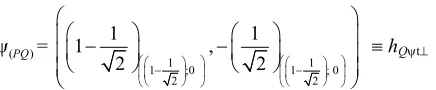
4.2. Paraquantum Entanglement in the Interaction between Two Equally Physical Bodies or Particles

In the process of Paraquantum logical Entangl the information from measurements performed on th

rvable Variables on the physical environment [1 the paraquantum anal

there are two symmetric Lattices where the values of measurements represented through the equality of values μA = λB andμB = λA will simultaneously compound two pairs related to two Paraquantum Logical states ψA = (DC,

Dct) and ψB = (–DC,Dct) resulting in Certainty Degrees

Module of the Vectors of State MP(ψ) will have the same simultaneous variations and the two resulting values of Intensity Degrees of the Real logical state μψRA and μψRB will have symmetry with respect to the Indefinition value 0.5.

In the paraquantum analysis, the entanglement of two Systems takes into account two symmetric Lattices which are in the same Universe of Discourse in only one Fun- damental Lattice. Since the variations of the measure- ments on t

ysical environment, they are reflected into the Lattice of States through the values of the Evidence Degrees μ and λ and their intensities depend on the scale or on the Interval of Interest considered. So, every paraquantum analysis in the paraquantum universe is locally per- formed, being the Proposition logically negated and rep- resented on the side of the opposite Vertices that con-nects the axis of the certainty degrees. So, since the proposition (P1) of a system is the logical negation of the proposition of the other (P1), a variation in one of the measurements will instantly reflect on the symmetric values of the Intensity Degrees of the Real logical state of these two physical systems being analyzed. In case a Paraquantum Leap occurs due to the contradiction on the measurements from the side such that DC > 0 to the side such that DC < 0 on the physical system SA, then on the physical state SB a Paraquantum Leap will simultane- ously occur from the side such that DC < 0 to the side such that DC > 0. Figure 3 shows the entanglement of the information obtained from measurements performed on the Observable Variables on the physical environment S

that was divided in two physical systems SA and SB.

4.3. The Paraquantum Entanglement in the Interaction between Two Different Physical Bodies or Particles

The Paraquantum logical entanglement can be studie considering the Paraquantum Logical Model applie the effects that appear in the interaction among different

ical systems or particles in the physical environment. e the particles in this ca

take these differences into account in the Paraquantum analysis.

Initially we can consider for this study the interaction between two physical bodies A and B, where body A is represented by its Paraquantum Logical Model A, and this will be a reference. In the existence of the Paraquan- tum entangl

1-|DC| _-D CψRB

ψB = (-DC, Dct) P(ψ)B

DCψRA

F

P(ψ)A

1-|DC| Dct

ψA = (DC, Dct)



T

t

λ 1 0 1

μ

Certa

inty Degree

DC Dct Contradiction

Degree

+1

0

-1

+1 -1

λB= μA

Information Source 2

μB=λA

λi = 1 – μ2

Information Source 1 0.5

0.5

μA=λB λA =μB

Physical world

Measurements

Observable VariableB

Physical world

Measurements

[image:9.595.115.483.82.431.2]

Observable VariableA μ i = μ1

Figure 3. Paraquantum entanglement of information from measurements performed on observable variables which are linked to two identical physical systems SA and SB, but with propositions logically negated.

odel, the presence of body B changes the initial values

a- b-

taine ntum Logical Model

asses and in

to consider a second physical system and a Fundamental Lattice which involves both

gical M

body A and the external physical body B. In this condi- tion, for the Lattice of the reference Paraquantum Logical

observe that this interaction process appears in a natural way, since it is enough

M

and the paraquantum analysis will produce referenced values through the expansion.

4.4. The Universal Gravitational Constant and the Paraquantum Logic

In the interaction of different physical bodies on the P raquantum Entanglement, we observe that the values o

d on the Lattice of the Paraqua

of the reference body A can be related to the value of the Universal Gravitational constant G [12].

The Universal Gravitation Law proposed by Newton says that all objects are attracted to others with a force directly proportional to the product of their m

versely proportional to the square of the distance be- tween their centers. So, the most important physical phe- nomena of the observable universe are expressed in only one equation, showing that there are no differences be- tween the terrestrial and the celestial physics [13].

In the study of the Paraquantum Entanglement, we

systems is created. The Paraquantum analysis between two Lattices that represent the Paraquantum Lo

odels of Physical Systems shows that the paraquantum Entanglement occurs with the notion of distance and In- teraction Force among them. So, the value of a Paraquan- tum Gravitation Constantcan result from Quantization factors due to superposed Paraquantum Logical states which appear through the expansion of the Fundamental Lattice of the PQL. This natural process that occurs on the Paraquantum Logical Model identifies a resulting value of the Paraquantum Factor of quantization very close to the value established as the Universal Gravitational con- stant. We call this value Paraquantum Gravitational Con- stant Gψ. For a comparative study of values, first we pre-

sent how we obtained Newton’s Gravitational Constant

G through Kepler’s equations.

states and equations of Energy make the Law of Univer- sal Gravitation (UG) of Newton a mathematical tool of great interest to deal with physical phenomena and it was proposed from Kepler’s laws [12]. For the case of circu-

of the course, called normal acce

lar orbits, the inverse quadratic nature of the centripetal force can be easily computed from Kepler’s third law which is about the planetary movement and the dynamics of the uniform circular movement. According to Kepler’s third law, the square of the period T is proportional to the cube of the greater semi-axis of the ellipse. In the case of the circumference, the greater semi-axis is its own radius

R, then the mathematical expression for this statement is:

2 3

T KR (32) where: K is the proportionality constant.

In the study of the uniform circular movement (UCM) the velocity of the moving body does not vary in module, however constantly varies in direction [12]. The moving body has an acceleration which is directed to the center leration whose module is computed by:

2 n

v a

R

 (33)

Since the velocity v and the radius R in the Uniform Circular Movement have constant values, the module of the centripetal acceleration varies continuously because is directed from the object to the center of the circle.

2

π R ₍₃₄₎

2 4 c a T 

Multiplying both sides of the equation again by R2_{, we} have: 2 3 2 2 4π c R R a T 

Isolating the square of the period:

2 3 4π R

2 2 c T R a 

Rewriting, we have:

2 2 3 2 4π c T R R a     

  (35) the third Kepler’s

la estial es,

de 35).

This equation can be compared to

w for the study of the movements of cel bodi scribed by Equation (

2 3 4π

 

 _T2_

2 2 c T R R a     ↔

 

3 K R

From Equation (35) we obtain an important relation: 2

2 4π 3 c

R a  _T2 R

  (36) In the study of the planets it was observ d that the product of acceleration by the square of the radius R ap-

peared with a constant 2 _1.327

s c

K R a  .

:

e

Ks such that:

From where we can isolate the acceleration as follows

K 2 s c a R

 →ac 1.327₂

R 

at

The dynamics of the uniform Circular Movement (UCM) is such that, in a circular course, the force that we have to apply to the body is equal to the product of its mass by the normal acceleration, therefore from the equ-

ion that expresses Newton second law, we obtain:

c

Fma →ac F

m 

We can compare the equations: c 1.327₂

F a

m R

 

From where we obtain the force computed by:

2

R

This equation expresses t ravitati nal force that de- creases with the increase of R, known as the Force of the

sq ton, the gravitational

fo tional to

th the sun

performs a force

1 1.327

F   m

he g o

uare inverse. According to New

rce performed by the sun on a planet is propor e mass of the planet. By Newton’s third law, if

s

Fp on a planet, then the planet per- forms a force Fps on the sun, where he moduli of the fo

t

rces are equal: Fsp Fps. In order to find the gravita- tional constant in the study of interaction force between the planets, we must know the masses involved [12,13]. A proportionality constant was established which is in- dependent of any masses such that:

 

2 1 .327 1

ps p s

F m m

R   and 

 

2 1 1.327

sp s p

F m m

R    2 R and 1

ps p s

F  G m m

2 1

sp s p

F G m m

R

  

In the interaction between the two m ses, each one performs the half of the constant

as

Ks represented as a gravitational constant G. So, we have t e corresponding value of the Universal Gravitational Constant:

h

2 3 2

2π 1.327 _0.6635

2 2 s K R G T    

Henry Cavendish (1731-1810) performed the first measurements of G through the well known device called “Cavendish’s Scales”. The value of the Universal Gravi- tational constant accepted nowadays is [12-15]:

2 11

2 6.67 10 N m

G

Kg



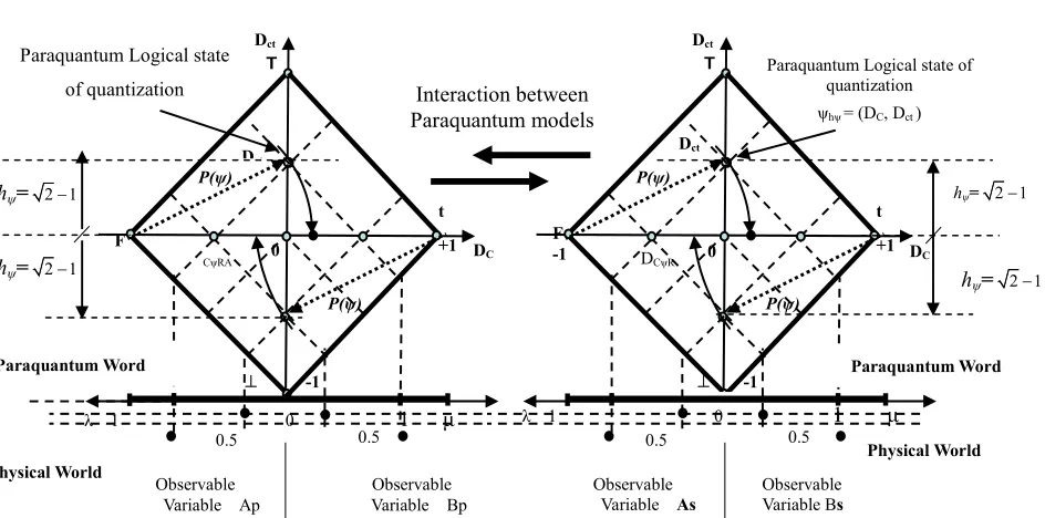
4.6. The Paraquantum Gravitational Constant Gψ

Th

[image:11.595.66.538.472.706.2]

As an example, we can observe from the following

Figure 4 that two bodies can be different in their physi- cal dimensions represented by two Lattices of the PQL

e ue expa Fundamental Lattice will be created. Accord-

.

e making reference to

is found to be considered as a phy- si

According to the properties of the PQL, the ne

lation to ea

e Paraquantum Gravitational constant Gψ appears on

the paraquantum analysis when we make an analogy be-tween the interaction of bodies or particles with the effect of Paraquantum Entanglement.

where, for the paraquantum analysis, there will always b an interaction between the two bodies in which a uniq

nded

ing to what was seen, the paraquantum analysis is always performed through a Lattice assigned to the PQL where the properties and forms of propagation of the Paraquan- tum Logical states ψ are analyzed

The propagation of the Paraquantum Logical state is characterized by the behavior and variation of the values of the Evidence Degrees extracted from the Observable Variables in the physical environment. The analysis on a Lattice is always done considering a proposition related to one only body. In this analysis, the body or physical system being studied always presents two or more phy- sical quantities which are considered as Observable Vari- ables from where we extract two Evidence Degrees: one favorable and another one unfavorabl

the proposition P.

In the practice the Evidence Degrees are normalized values and are in the closed real interval [0,1] where they are extracted from measurements established within an Interval of Interest or Universe of Discourse. So, when a

second physical body

cal system belonging to the Paraquantum analysis, the

PQL Lattice receives an expansion action that will cover both bodies in an interactive analysis. This is the effect of Paraquantum Entanglement applied to two bodies that may be different according to what will be considered in this study.

This natural Interaction for the paraquantum analysis causes both physical systems to interact creating a unique new Fundamental Lattice with all characteristics of nor- malizations and with Quantization factors of the indivi- dual Lattice.

w Lattice which is created by the interaction of the two bodies is bounded by the Region of Paraquantum Uncer- tainty. So, the interaction on the physical world between the two particles happens on the action line of the Para- quantum Gamma Factor γψ which delineates new equi-

librium points of the new fundamental Lattice.

The following Figure 5 shows this interaction of two individual Lattices and the creation of a unique Funda- mental Lattice from where, through a trigonometric pro- cess, we can obtain the resulting value of the Quantiza- tion Factor. When the values are considered in re

ch one the individual Lattices, the bounds of the new Fundamental Lattice expanded by the interaction of the two physical systems will increase equilibrium points.

This effect causes the resulting value of the Quantiza- tion Factor, for the reference taken from the Lattice of each individual physical System, to be an aggregation of values given by:





ψexpan ψ ψ

Valueh   _1 1 h _h (37)

Interaction Paraquantu

between m models

hψ= 2 1

hψ= 2 1

Observable Variable Ap

hψ= 2 1

CψRA Paraquantum Logical state

of quantization

 -1 Dct

Dct

0 DC Dt

t

+1

T

P(ψ)

λ 1 0 1 μ

0.5 0.5

F

P(ψ)

Physical World

Observable Variable Bp

Paraquantum Word

Observable Variable As

hψ= 2 1

DCψR

Paraquantum Logical state of quantization

ψhψ= (DC, Dct )



-1

0 DC Dct

t

+1

T

P(ψ)

λ 1 0 1 μ

0.5 0.5

F -1

P(ψ)

Physical World Paraquantum Word

Observable Variable Bs

Figure 4. Two Lattices of the PQL representing two different physical systems or an interaction that will mandatorily be

1 



1 h







1 1 h h

   

 





1 1 h h

     hψ= 2 1

Paraquantum Logical state of

quantization

ψhψ= (DC, Dct )



Dct

1 Dct

T

P(ψ)

λ 1 00.5

Referencial

F

P(ψ)

Observable Variable A,C

hψ= 2 1



Dct

1

0 DCpS Dct

t +1

T

P(ψ)

μ

0.5

P(ψ)

Observable Variable B,D

DctpS

+1

Paraquantum Logical state of quantization

ψhψ= (DC, Dct )

P(ψ)

Physical World

Paraquantum Word

[image:12.595.114.494.86.406.2]

Physical World Paraquantum Word

Figure 5. Both Lattices of the PQL representing two physical systems whose interaction generates a unique expanded Fun-

damental Lattice.

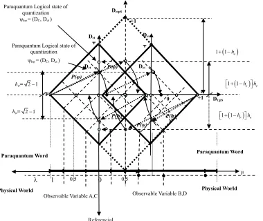
where: h 4.7. The Paraquantum Logical Model for

Interaction of Several and Different Particles

Through the paraquantum analysis we can study the in- teraction of particles where the representing Lattices of each physical body are considered in only one set formed by Paraquantum Logical models capable of modeling complex physical systems.

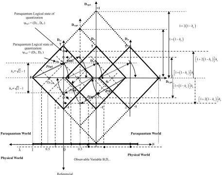
Figure 6 shows the example of the interaction of three systems forming only one expanded Fundamental Lattice such that the study takes into account the Lattice on the left as the referential one.

For this condition, where the reference of values is considered from the Lattice of each individual physical System, we have the resulting value of the Paraquantum Factor of quantization for this type of Paraquantum En- tanglement of three Lattices, resulting in an aggregation

side Lattice is computed by:  is the Paraquantum Factor of quantization.

ψexpan

Valueh = Resulting Value of the Paraquantum Factor of quantization expanded by the interaction of the

o physical systems computed by the individual Lattice. tw

As: hψ 2 1 , then, computing the value of the

Quan-ion Factor in an aggregatQuan-ion of values obtained by the interaction of the two Lattices, as Equation (37) shows, we have:

tizat







1





2 1



 _  _

 

 

0.656854249

Being an expansion value due to the interaction caused by the presence of another body in the analysis, we call this value Factor of Constant of Paraquantum Gravitation

Gψ, such that for the interaction of two bodies, we have:



ψ



ψ

1 1

G   _ h _h (38)

ψexpan

Valueh   1 1 2

→ Valuehψexpan 



Since: hψ



2 1



, from Equation (38) the value of

the constant of Paraquantum Gravitation results:













1 1 2 1 2 1

G_   _  _ 

 

0.656854249

G 





ψe xpan3 ψ ψ

Valueh 1 2 1 h h

of values on the vertical axis of the Lattice on the left. This value shown on the vertical axis of the left-hand

 

DctpS

+1

Physical World

Paraquantum World

1 2 1  h

 

1 1 h

1 2 1 _ h_h

 

1 1 h h

  

 

1 1 hh

1 2 1  hh hψ= 2 1

DCψR

Paraquantum Logical state of quantization

ψhψ1 = (DC, Dct )

Dct

 -1

Dt

T

P(ψ)

λ 1 0 0.5

Referencial

F

P(ψ)

Paraquantum World

hψ= 2 1

 Dct

-1

0 DCpS

Dct

t 1

T

P(ψ)

μ

0.5

P(ψ)

Observable Variable B,D,..

DctpS

Paraquantum Logical state of quantization

ψhψ3 = (DC, Dct )

P(ψ)

Dct

 -1

T

[image:13.595.69.528.85.445.2]

Physical World

Figure 6. The three Lattices of the PQL representing three physical systems whose interaction form a unique Fundamental

Lattice expanded.

ψ

h is the Paraquantum Factor of quantization.

ψexpan3

Valorh = resulting value of the Paraquantum Factor of quantization expanded by the interaction of the three physical systems computed by the individual left-hand side Lattice.

As in the Fundamental Lattice hψ



2 1



so the

new value of the Pa Factor of quantization obtained by the interacti hree Lattices accord- ing to Equation (39) i

raquantum on of the t s:













Valueh  _1 2 1 2 1 _ 2 1

4872

e consider the interaction

am fect of the Paraquantum

Entanglement where the value of the Factor of uantum Quantization is obtained in this way, the Paraq-uantum analysis can be expressed by the notion of

dis-Systems with the value of the constant

K that related the Interaction Force in charged particles studied with Coulomb’s Law.

4.8. The Paraquantum Universe Model

The analysis of complex physical systems represented by several Lattices forming an interlaced net can be identi- fied as a model of Paraquantum universe. Based in the figures, if the reference Lattice is the Paraquantum Lat- tice represented to the left of the group, the equation to compute the value on the vertical axis is:

For two Lattices N = 2:

 



2



ψexpan 2 ψ ψ ψ

Valueh N h  h  h

ψexpan3

→Valueh_ψexpan30.899 We observe that when w

ong different particles as an ef

tance among the bodies. So, we can make an analogy of the value obtained as the Paraquantum Entanglement of the three Physical



 

 







2

ψexpan 2

Valueh _N  2 1 _ 2 1  2 1 _

 

ψexp an 2

Valueh N 0.656854324 For three Lattices N = 3:

ψexpan3 ψ ψ ψ



 

 



ψexpan3

alueh  2 1 2_ 2 1  2 1 2

V  



 

2



ψ hψ

ψexpan3

Valueh 0.899495049 For four Lattices N = 4:



ψexpan 4 ψ

Valueh N h 3 h



 

 



2

ψexpan 4

Valueh  2 1 3_ 2 1  2 1 _

Valueh 1.142135774

of Lattices the equation is: 2

exp anN N 31). This makes with ged and it

ch pair of Lat-

tic sical bodies, a new third one

will be formed as a paraquantum agglutinatoer. So, the agglutinating Lattice will be the reference one and its position will be the middle of the Fundamental Lattice. In this analysis, the value of the Paraquantum Factor of quantization will be expressed in relation to the Funda- mental Lattice that will be subject to a contraction pro-

ce studied in the Paraquantum

Logical Model (see [17,18]).

5. Conclusion

In this paper, we presented a study about the Paraq - tum Entanglement covering similar and dif nt systems where the values related to the interaction mong bodies or physical particles were established. The obtained re- sults produce large possibilities for new researches where Paraquantum Logics is a good option to serve as a base for models of physical models interconnecting through the paraquantum universe several areas of physics which nowadays have results which are not compatible. researches about resulting values of the interactions of

different bodies in the form of the Paraquantum Entan- glement can lead to deeper studies that will produce mo-

de such as in

co tion about

the interactions among particles used in the model of nuclear physics.

ψexpan4 For an amount N







 



ψexp an ψ ψ ψ

Valueh _{N N} h  N1 h  h (40)

ψ

h is the Paraquantum Factor of quantization.

ψexp an

Valorh _N = resulting value of the Paraquantum Factor of quantization expanded by the interaction of N

physical systems computed by the individual left-hand side Lattice. where: N is the number of Paraquantum Lattices of the group.

However, when the number of Lattices of the group will be greater that 3 (N > 3) the calculated value will be greater that 1 ( Valorh_ψ

that the reference Lattice of the group is chan passes to be the next Lattice to the right.

The idea of the contracted model, where the Funda- mental Lattice aggregates or receives smaller Lattices in its inner side, makes us consider a notion of mass or for- mation of matter in the paraquantum analysis. So, the Paraquantum Entanglement in the analysis of Physical Systems is about the process where, for ea

es representing two phy

ss according to what was

uan fere

a

The

ls that deal with interactions of large masses smology and also can lead to a new concep

standard

REFERENCES

[1] S. Jas’kowski, “Propositional Calculus for Contradictory Deductive Systems,” Studia Logica, Vol. 24, No. 1, 1969, pp. 143-157. doi:10.1007/BF02134311

[2] N. C. A. Da Costa, “On the Theory of Inconsistent For-mal Systems,” Notre Dame Journal of Formal Logic, Vol. 15, No. 4, 1974, pp. 497-510.

doi:10.1305/ndjfl/1093891487

[3] N. C. A. Da Costa and D. Marconi, “An Overview of Pa- raconsistent Logic in the 80’s,” The Journal of Non-Classical Logic, Vol. 6, 1989, pp. 5-31.

[4] N. C. A. Da Costa, V. S. Subrahmanian and C. Vago, “The Paraconsistent Logic PT,” Zeitschrift fur Mathe- matische Logik und Grundlagen der Mathematik, Vol. 37, No. 9-12, 1991, pp. 139-148.

doi:10.1002/malq.19910370903

[5] J. I. Da Silva Filho, G. Lambert-Torres and J. M. Abe “Uncertainty Treatment Using Paraconsistent Logic—In- troducing Paraconsistent Artificial Neural Networks,” Vol. 21, IOS Press, Amsterdam, 2010.

[6] J. I. Da Silva Filho, G. Lambert-Torres, L. F. P. Ferrara, A. M. C. Mário, M. R. Santos, A. S. Onuki, J. M. Camargo and A. Rocco, “Paraconsistent Algorithm Ex-tractor of Contradiction Effects—Paraextrctr,” Journal of

Software Engineering and Applications, Vol. 4, No. 1, 2011, pp. 579-584. doi:10.4236/jsea.2011.410067

Filho, A. Rocco, A. S. Onuki, L. F. P. M. Camargo, “Electric Power Systems [7] J. I. Da Silva

Ferrara and J.

Contingencies Analysis by Paraconsistent Logic Applica-tion,” International Conference on Intelligent Systems Applications to Power Systems, Santa Cecilia, 5-8 No-vember 2007, pp. 1-6,

doi:10.1109/ISAP.2007.4441603

[8] C. A. Fuchs and A. Peres, “Quantum Theory Needs No ‘Interpretation’,” Physics Today, Vol. 53, No. 3, 2000, pp. 70-71. doi:10.1063/1.883004

[9] D. Krause and O. Bueno, “Scientific Theories, Models, and the Semantic Approach,” Principia, Vol. 11, No. 2, 2007, pp. 187-201.

[10] J. I. Da Silva Filho, “Paraconsistent Annotated Logic in analysis of Physical Systems: Introducing the Paraquan-tum Factor of quantization hψ,” Journal of Modern Phy-

sics, Vol. 2, No. 1, 2011, pp. 1397-1409. doi:10.4236/jmp.2011.211172

[11] J. I. Da Silva Filho, “A Paraconsistent Annotated

nalysis of Physical Systems with Logic: Introducing the Para- quantum Gamma Factor γ,” Journal of Modern Physics, Vol. 2, No. 1,

doi:10.4236/jm

ψ

, “Physics for Scientists,” nd Company, New York,

ew York, 2007.

/PhysRev.47.777 [12] J. P. Mckelvey and H. Grotch, “Physics for Science and

Engineering,” Harper and Row Publisher, Inc., New York, London, 1978.

[13] Pl. A. Tipler, “Physics,” Worth Publishers Inc., New York, 1976.

[14] Pl. A. Tipler and G. M. Tosca 6th Edition, W. H. Freeman a 2007.

[15] Pl. A. Tipler and R. A. Llewellyn, “Modern Physics,” 5th Edition, W. H. Freeman and Company, N

[16] A. Einstein, B. Podolsky and N. Rosen, “Can

Quan-tum-Mechanical Description of Physical Reality Be Con-sidered Complete?” Physical Review, Vol. 47, No. 10, 1935, pp. 777-780. doi:10.1103

[17] J. I. Da Silva Filho, “Analysis of the Spectral Line Emis-sions of the Hydrogen Atom with Paraquantum Logic,” Journal of Modern Physics, Vol. 3, No. 3, 2012, pp. 233-254. doi:10.4236/jmp.2012.33033

[18] J. I. Da Silva Filho, “An Introductory Study of the Hy-drogen Atom with Paraquantum Logic,” Journal of Mo- dern Physics, Vol. 3, No. 4, 2012, pp. 312-333