Proceedings of NAACL-HLT 2018, pages 355–364
Classical Structured Prediction Losses for Sequence to Sequence Learning
Sergey Edunov∗, Myle Ott∗,
Michael Auli, David Grangier, Marc’Aurelio Ranzato
Facebook AI Research
Menlo Park, CA and New York, NY
Abstract
There has been much recent work on train-ing neural attention models at the sequence-level using either reinforcement learning-style methods or by optimizing the beam. In this paper, we survey a range of classical objec-tive functions that have been widely used to train linear models for structured prediction and apply them to neural sequence to se-quence models. Our experiments show that these losses can perform surprisingly well by slightly outperforming beam search optimiza-tion in a like for like setup. We also report new state of the art results on both IWSLT’14 German-English translation as well as Giga-word abstractive summarization. On the large WMT’14 English-French task, sequence-level training achieves 41.5 BLEU which is on par with the state of the art.1
1 Introduction
Sequence to sequence models are usually trained with a simple token-level likelihood loss (Sutskever et al., 2014; Bahdanau et al., 2014). However, at test time, these models do not pro-duce a single token but a whole sequence. In order to resolve this inconsistency and to potentially improve generation, recent work has focused on training these models at the sequence-level, for instance using REINFORCE (Ranzato et al., 2015), actor-critic (Bahdanau et al.,2016), or with beam search optimization (Wiseman and Rush, 2016).
Before the recent work on sequence level train-ing for neural networks, there has been a large body of research on training linear models at the
∗Equal contribution.
1An implementation of the losses is available
as part of fairseq at https://github.com/ facebookresearch/fairseq-py/tree/
classic_seqlevel
sequence level. For example, direct loss opti-mization has been popularized in machine transla-tion with the Minimum Error Rate Training algo-rithm (MERT; Och 2003) and expected risk min-imization has an extensive history in NLP (Smith and Eisner,2006;Rosti et al.,2010;Green et al., 2014). This paper revisits several objective func-tions that have been commonly used for structured prediction tasks in NLP (Gimpel and Smith,2010) and apply them to a neural sequence to sequence model (Gehring et al., 2017b) (§2). Specifically, we consider likelihood training at the sequence-level, a margin loss as well as expected risk train-ing. We also investigate several combinations of global losses with token-level likelihood. This is, to our knowledge, the most comprehensive com-parison of structured losses in the context of neural sequence to sequence models (§3).
We experiment on the IWSLT’14 German-English translation task (Cettolo et al., 2014) as well as the Gigaword abstractive summarization task (Rush et al., 2015). We achieve the best re-ported accuracy to date on both tasks. We find that the sequence level losses we survey perform similarly to one another and outperform beam search optimization (Wiseman and Rush,2016) on a comparable setup. On WMT’14 English-French, we also illustrate the effectiveness of risk mini-mization on a larger translation task. Classical losses for structured prediction are still very com-petitive and effective for neural models (§5,§6).
2 Sequence to Sequence Learning
The general architecture of our sequence to se-quence models follows the encoder-decoder ap-proach with soft attention first introduced in ( Bah-danau et al., 2014). As a main difference, in most of our experiments we parameterize the en-coder and the deen-coder as convolutional neural
networks instead of recurrent networks (Gehring et al., 2017a,b). Our use of convolution is mo-tivated by computational and accuracy considera-tions. However, the objective functions we present are model agnostic and equally applicable to re-current and convolutional models. We demon-strate the applicability of our objective functions to recurrent models (LSTM) in our comparison to Wiseman and Rush(2016) in§6.6.
Notation. We denote the source sentence asx, an
output sentence of our model asu, and the
refer-ence ortargetsentence ast. For some objectives,
we choose a pseudo referenceu∗ instead, such as
a model output with the highest BLEU or ROUGE score among a set of candidate outputs,U, gener-ated by our model.
Concretely, the encoder processes a source sen-tencex = (x1, . . . , xm)containingmwords and outputs a sequence of states z = (z1. . . . , zm). The decoder takesz and generates the output
se-quenceu= (u1, . . . , un)left to right, one element at a time. For each output ui, the decoder
com-putes hidden state hi based on the previous state
hi−1, an embedding gi−1 of the previous target
language word ui−1, as well as a conditional
in-putci derived from the encoder outputz. The at-tention contextci is computed as a weighted sum of (z1, . . . , zm) at each time step. The weights of this sum are referred to as attention scores and allow the network to focus on the most relevant parts of the input at each generation step. Atttion scores are computed by comparing each en-coder statezjto a combination of the previous de-coder statehi and the last predictionui; the result is normalized to be a distribution over input ele-ments. At each generation step, the model scores for the V possible next target words ui by trans-forming the decoder output hi via a linear layer with weights Wo and bias bo: si = Wohi +bo. This is turned into a distribution via a softmax:
p(ui|u1, . . . , ui−1,x) = softmax(si).
Our encoder and decoder use gated convolu-tional neural networks which enable fast and accu-rate generation (Gehring et al.,2017b). Fast gener-ation is essential to efficiently train on the model output as is done in this work as sequence-level losses require generating at training time. Both en-coder and deen-coder networks share a simple block structure that computes intermediate states based on a fixed number of input tokens and we stack several blocks on top of each other. Each block
contains a 1-D convolution that takes as input k
feature vectors and outputs another vector; sub-sequent layers operate over thekoutput elements
of the previous layer. The output of the convolu-tion is then fed into a gated linear unit (Dauphin et al., 2017). In the decoder network, we rely on causal convolution which rely only on states from the previous time steps. The parametersθof
our model are all the weight matrices in the en-coder and deen-coder networks. Further details can be found inGehring et al.(2017b).
3 Objective Functions
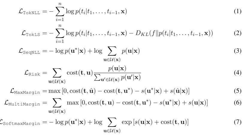
We compare several objective functions for train-ing the model architecture described in §2. The corresponding loss functions are either computed over individual tokens (§3.1), over entire se-quences (§3.2) or over a combination of tokens and sequences (§3.3). An overview of these loss functions is given in Figure1.
3.1 Token-Level Objectives
Most prior work on sequence to sequence learning has focused on optimizing token-level loss func-tions, i.e., functions for which the loss is computed additively over individual tokens.
Token Negative Log Likelihood (TokNLL) Token-level likelihood (TokNLL, Equation 1) minimizes the negative log likelihood of individ-ual reference tokens t = (t1, . . . , tn). It is the most common loss function optimized in related work and serves as a baseline for our comparison. Token NLL with Label Smoothing (TokLS) Likelihood training forces the model to make ex-treme zero or one predictions to distinguish be-tween the ground truth and alternatives. This may result in a model that is too confident in its training predictions, which may hurt its generalization per-formance. Label smoothing addresses this by act-ing as a regularizer that makes the model less con-fident in its predictions. Specifically, we smooth the target distribution with a prior distribution f
that is independent of the current inputx(Szegedy
et al., 2015;Pereyra et al.,2017; Vaswani et al., 2017). We use a uniform prior distribution over all words in the vocabulary,f = V1. One may also
LTokNLL =−
n
X
i=1
logp(ti|t1, . . . , ti−1,x) (1)
LTokLS=− n
X
i=1
logp(ti|t1, . . . , ti−1,x)−DKL(fkp(ti|t1, . . . , ti−1,x)) (2)
LSeqNLL =−logp(u∗|x) + log X
u∈U(x)
p(u|x) (3)
LRisk= X
u∈U(x)
cost(t,u)P p(u|x)
u0∈U(x)p(u0|x)
(4)
LMaxMargin= max [0,cost(t,uˆ)−cost(t,u∗)−s(u∗|x) +s(ˆu|x)] (5)
LMultiMargin= X
u∈U(x)
max [0,cost(t,u)−cost(t,u∗)−s(u∗|x) +s(u|x)] (6)
LSoftmaxMargin =−logp(u∗|x) + log X
u∈U(x)
[image:3.595.122.528.71.301.2]exp [s(u|x) + cost(t,u)] (7)
Figure 1: Token and sequence negative log-likelihood (Equations1 and3), token-level label smoothing (Equa-tion2), expected risk (Equation4), max-margin (Equation5), multi-margin (Equation6), softmax-margin (Equa-tion7). We denote the source asx, the reference target ast, the set of candidate outputs asUand the best candidate (pseudo reference) asu∗. For max-margin we denote the candidate with the highest model score asuˆ.
p(u|x) to the negative log likelihood (TokLS, Equation 2). In practice, we implement label smoothing by modifying the ground truth distribu-tion for worduto beq(u) = 1−andq(u0) = V
for u0 6= u instead of q(u) = 1 andq(u0) = 0
whereis a smoothing parameter.
3.2 Sequence-Level Objectives
We also consider a class of objective functions that are computed over entire sequences, i.e., sequence-level objectives. Training with these objectives requires generating and scoring multi-ple candidate output sequences for each input se-quence during training, which is computationally expensive but allows us to directly optimize task-specific metrics such as BLEU or ROUGE.
Unfortunately, these objectives are also typi-cally defined over the entire space of possible out-put sequences, which is intractable to enumerate or score with our models. Instead, we compute our sequence losses over a subset of the output space,U(x), generated by the model. We discuss
approaches for generating this subset in§4.
Sequence Negative Log Likelihood (SeqNLL) Similar toTokNLL, we can minimize the negative log likelihood of an entire sequence rather than in-dividual tokens (SeqNLL, Equation3). The
log-likelihood of sequenceu is the sum of individual
token log probabilities, normalized by the number of tokens to avoid bias towards shorter sequences:
p(u|x) = exp1 n
n
X
i=1
logp(ui|u1, . . . , ui−1,x)
As target we choose a pseudo reference2amongst
the candidates which maximizes either BLEU or ROUGE with respect tot, the gold reference:
u∗(x) = arg max
u∈U(x)
BLEU(t,u)
As is common practice when computing BLEU at the sentence-level, we smooth all initial counts to one (except for unigram counts) so that the geo-metric mean is not dominated by zero-valued n -gram match counts (Lin and Och,2004).
Expected Risk Minimization (Risk)
This objective minimizes the expected value of a given cost function over the space of candidate se-quences (Risk, Equation4). In this work we use task-specific cost functions designed to maximize BLEU or ROUGE (Lin,2004), e.g.,cost(t,u) = 2Another option is to use the gold reference target,t, but
1−BLEU(t,u), for a given a candidate sequence
u and targett. Different toSeqNLL(§3.2), this loss may increase the score of several candidates that have low cost, instead of focusing on a sin-gle sequence which may only be marginally bet-ter than any albet-ternatives. Optimizing this loss is a particularly good strategy if the reference is not always reachable, although compared to classical phrase-based models, this is less of an issue with neural sequence to sequence models that predict individual words or even sub-word units.
The Risk objective is similar to the REIN-FORCE objective used in Ranzato et al. (2015), since both objectives optimize an expected cost or reward (Williams,1992). However, there are a few important differences: (1) whereas REINFORCE typically approximates the expectation with a sin-gle sampled sequence, theRiskobjective consid-ers multiple sequences; (2) whereas REINFORCE relies on abaseline reward3 to determine the sign
of the gradients for the current sequence, for the Riskobjective we instead estimate the expected cost over a set of candidate output sequences (see §4); and (3) while the baseline reward is different for every word in REINFORCE, the expected cost is the same for every word in risk minimization since it is computed on the sequence level based on the actual cost.
Max-Margin
MaxMargin (Equation 5) is a classical margin loss for structured prediction (Taskar et al.,2003; Tsochantaridis et al.,2005) which enforces a mar-gin between the model scores of the highest scor-ing candidate sequence uˆ and a reference
se-quence. We replace the human referencetwith a
pseudo-referenceu∗ since this setting performed
slightly better in early experiments;u∗ is the
can-didate sequence with the highest BLEU score. The size of the marginvariesbetween samples and is given by the difference between the cost ofu∗and
the cost of uˆ. In practice, we scale the margin by a hyper-parameterβdetermined on the
valida-tion set:β(cost(t,uˆ)−cost(t,u∗)). For this loss
we use the unnormalized scores computed by the model before the final softmax:
s(u|x) = 1 n
n
X
i=1
s(ui|u1, . . . , ui−1,x)
3Ranzato et al. (2015) estimate the baseline reward
for REINFORCE with a separate linear regressor over the model’s current hidden state.
Multi-Margin
MaxMargin only updates two elements in the candidate set. We therefore consider MultiMargin (Equation 6) which enforces a margin betweeneverycandidate sequenceuand a reference sequence (Herbrich et al., 1999), hence the name Multi-Margin. Similar toMaxMargin, we replace the reference t with the
pseudo-referenceu∗.
Softmax-Margin
Finally, SoftmaxMargin (Equation 7) is an-other classic loss that has been proposed by Gim-pel and Smith(2010) as another way to optimize task-specific costs. The loss augments the scores inside theexpofSeqNLL(Equation3) by a cost. The intuition is that we want to penalize high cost outputs proportional to their cost.
3.3 Combined Objectives
We also experiment with two variants of combin-ing sequence-level objectives (§3.2) with token-level objectives (§3.1). First, we consider a weighted combination (Weighted) of both a sequence-level and token-level objective (Wu et al.,2016), e.g., forTokLSandRiskwe have:
LWeighted =αLTokLS+ (1−α)LRisk (8)
where α is a scaling constant that is tuned on a
held-out validation set.
Second, we consider a constrained combina-tion (Constrained), where for any given in-put we use either the token-level or sequence-level loss, but not both. The motivation is to main-tain good token-level accuracy while optimizing on the sequence-level. In particular, a sample is processed with the sequence loss if the token loss under the current model is at least as good as the token loss of a baseline modelLb
TokLS. Otherwise, we update according to the token loss:
LConstrained= (
LRisk LTokLS≤ Lb TokLS LTokLS otherwise
(9) In this work we use a fixed baseline model that was trained with a token-level loss to convergence.
score with our models. We therefore use a subset ofKcandidate sequencesU(x) ={u1, . . . , uK}, which we generate with our models.
We consider two search strategies for generat-ing the set of candidate sequences. The first is
beam search, a greedy breadth-first search that maintains a “beam” of the top-K scoring
candi-dates at each generation step. Beam search is the
de factodecoding strategy for achieving state-of-the-art results in machine translation. The second strategy is sampling (Chatterjee and Cancedda, 2010), which producesK independent output
se-quences by sampling from the model’s conditional distribution. Whereas beam search focuses on high probability candidates, sampling introduces more diverse candidates (see comparison in§6.5). We also consider both online and offline candi-date generation settings in§6.4. In the online set-ting, we regenerate the candidate set every time we encounter an input sentencexduring training. In
the offline setting, candidates are generated before training and are never regenerated. Offline gen-eration is also embarrassingly parallel because all samples use the same model. The disadvantage is that the candidates become stale. Our model may perfectly be able to discriminate between them af-ter only a single update, hindering the ability of the loss to correct eventual search errors.4
Finally, while some past work has added the ref-erence target to the candidate set, i.e., U0(x) =
U(x) ∪ {t}, we find this can destabilize train-ing since the model learns to assign low proba-bilities nearly everywhere, ruining the candidates generated by the model, while still assigning a slightly higher score to the reference (cf. Shen et al.(2016)). Accordingly we do not add the ref-erence translation to our candidate sets.
5 Experimental Setup
5.1 Translation
We experiment on the IWSLT’14 German to En-glish (Cettolo et al., 2014) task using a similar setup as Ranzato et al. (2015), which allows us to compare to other recent studies that also adopted this setup, e.g., Wiseman and Rush(2016).5 The
training data consists of 160K sentence pairs and the validation set comprises 7K sentences
ran-4We can mitigate this issue by regenerating infrequently,
i.e., once everybbatches but we leave this to future work.
5Different toRanzato et al.(2015) we train on sentences
of up to 175 rather than 50 tokens.
domly sampled and held-out from the train data. We test on the concatenation oftst2010, tst2011, tst2012, tst2013 anddev2010which is of similar size to the validation set. All data is lowercased and tokenized with a byte-pair encoding (BPE) of 14,000 types (Sennrich et al.,2016) and we evalu-ate with case-insensitive BLEU.
We also experiment on the much larger WMT’14 English-French task. We remove sen-tences longer than 175 words as well as pairs with a source/target length ratio exceeding 1.5 resulting in 35.5M sentence-pairs for training. The source and target vocabulary is based on 40K BPE types. Results are reported on both newstest2014 and a validation set held-out from the training data com-prising 26,658 sentence pairs.
We modify thefairseq-py toolkit to implement the objectives described in §3.6 Our translation
models have four convolutional encoder layers and three convolutional decoder layers with a kernel width of 3 and 256 dimensional hidden states and word embeddings. We optimize these mod-els using Nesterov’s accelerated gradient method (Sutskever et al., 2013) with a learning rate of 0.25 and momentum of 0.99. Gradient vectors are renormalized to norm 0.1 (Pascanu et al.,2013).
We train our baseline token-level models for 200 epochs and then anneal the learning by shrink-ing it by a factor of 10 after each subsequent epoch until the learning rate falls below 10−4.
All sequence-level models are initialized with pa-rameters of a token-level model before anneal-ing. We then train sequence-level models for an-other 10 to 20 epochs depending on the objective. Our batches contain 8K tokens and we normal-ize gradients by the number of non-padding to-kens per mini-batch. We use weight normalization for all layers except for lookup tables (Salimans and Kingma,2016). Besides dropout on the em-beddings and the decoder output, we also apply dropout to the input of the convolutional blocks at a rate of 0.3 (Srivastava et al., 2014). We tuned the various parameters above and report accuracy on the test set by choosing the best configuration based on the validation set.
We length normalize all scores and probabili-ties in the sequence-level losses by dividing by the number of tokens in the sequence so that scores are comparable between different lengths.
ditionally, when generating candidate output quences during training we limit the output se-quence length to be less than 200 tokens for ef-ficiency. We generally use 16 candidate sequences per training example, except for the ablations where we use 5 for faster experimental turnaround.
5.2 Abstractive Summarization
For summarization we use the Gigaword corpus as training data (Graff et al.,2003) and pre-process it identically toRush et al.(2015) resulting in 3.8M training and 190K validation examples. We evalu-ate on a Gigaword test set of 2,000 pairs identical to the one used byRush et al. (2015) and report F1 ROUGE similar to prior work. Our results are in terms of three variants of ROUGE (Lin,2004), namely, ROUGE-1 (RG-1, unigrams), ROUGE-2 (RG-2, bigrams), and ROUGE-L (RG-L, longest-common substring). Similar toAyana et al.(2016) we use a source and target vocabulary of 30k words. Our models for this task have 12 layers in the encoder and decoder each with 256 hidden units and kernel width 3. We train on batches of 8,000 tokens with a learning rate of 0.25 for 20 epochs and then anneal as in§5.1.
6 Results
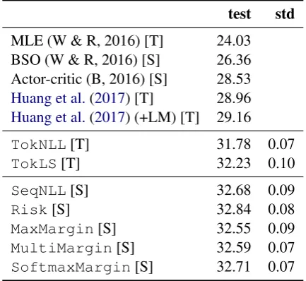
6.1 Comparison of Sequence Level Losses First, we compare all objectives based on a weighted combination with token-level label smoothing (Equation 8). We also show the like-lihood baseline (MLE) of Wiseman and Rush (2016), their beam search optimization method (BSO), the actor critic result of Bahdanau et al. (2016) as well as the best reported result on this dataset to date byHuang et al.(2017). We show a like-for-like comparison to Wiseman and Rush (2016) with a similar baseline model below (§6.6). Table1shows that all sequence-level losses out-perform level losses. Our baseline token-level results are several points above other figures in the literature and we further improve these re-sults by up to 0.61 BLEU withRisktraining.
6.2 Combination with Token-Level Loss Next, we compare various strategies to com-bine sequence-level and token-level objectives (cf. §3.3). For these experiments we use 5 candi-date sequences per training example for faster ex-perimental turnaround. We consider Risk as
test std MLE (W & R, 2016) [T] 24.03 BSO (W & R, 2016) [S] 26.36 Actor-critic (B, 2016) [S] 28.53 Huang et al.(2017) [T] 28.96 Huang et al.(2017) (+LM) [T] 29.16
TokNLL[T] 31.78 0.07
TokLS[T] 32.23 0.10
SeqNLL[S] 32.68 0.09
Risk[S] 32.84 0.08
MaxMargin[S] 32.55 0.09
MultiMargin[S] 32.59 0.07
[image:6.595.308.525.63.262.2]SoftmaxMargin[S] 32.71 0.07
Table 1: Test accuracy in terms of BLEU on IWSLT’14 German-English translation with various loss functions cf. Figure 1. W & R (2016) refers toWiseman and Rush(2016), B (2016) toBahdanau et al.(2016), [S] indicates sequence level-training and [T] token-level training. We report averages and standard deviations over five runs with different random initialization.
valid test
TokLS 33.11 32.21
Riskonly 33.55 32.45
Weighted 33.91 32.85
Constrained 33.77 32.79
Random 33.70 32.61
Table 2: Validation and test BLEU for loss combina-tion strategies. We either use token-levelTokLSand sequence-levelRiskindividually or combine them as a weighted combination, a constrained combination, a random choice for each sample, cf.§3.3.
sequence-level loss and label smoothing as token-level loss. Table2shows that combined objectives perform better than pure Risk. The weighted combination (Equation 8) with α = 0.3
per-forms best, outperforming constrained combina-tion (Equacombina-tion9). We also compare to randomly choosing between token-level and sequence-level updates and find it underperforms the more princi-pled constrained strategy. In the remaining exper-iments we use the weighted strategy.
6.3 Effect of initialization
valid test
TokNLL 32.96 31.74
Riskinit withTokNLL 33.27 32.07
∆ +0.31 +0.33
TokLS 33.11 32.21
Riskinit withTokLS 33.91 32.85
[image:7.595.82.281.64.176.2]∆ +0.8 +0.64
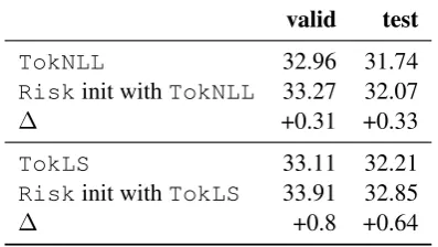
Table 3: Effect of initializing sequence-level training (Risk) with parameters from token-level likelihood (TokNLL) or label smoothing (TokLS).
[image:7.595.309.520.65.222.2]valid test Online generation 33.91 32.85 Offline generation 33.52 32.44
Table 4: Generating candidates online or offline.
achieves 0.7-0.8 better BLEU compared to initial-izing with parameters from token-level likelihood. The improvement of initializing withTokNLLis only 0.3 BLEU with respect to theTokNLL base-line, whereas, the improvement from initializing withTokLSis 0.6-0.8 BLEU. We believe that the regularization provided by label smoothing leads to models with less sharp distributions that are a better starting point for sequence-level training.
6.4 Online vs. Offline Candidate Generation Next, we consider the question if refreshing the candidate subset at every training step (online) results in better accuracy compared to generat-ing candidates before traingenerat-ing and keepgenerat-ing the set static throughout training (offline). Table4shows that offline generation gives lower accuracy. How-ever the online setting is much slower, since re-generating the candidate set requires incremental (left to right) inference with our model which is very slow compared to efficient forward/backward over large batches of pre-generated hypothesis. In our setting, offline generation has 26 times higher throughput than the online generation setting, de-spite the high inference speed of fairseq (Gehring et al.,2017b).
6.5 Beam Search vs. Sampling and Candidate Set Size
So far we generated candidates with beam search, however, we may also sample to obtain a more di-verse set of candidates (Shen et al., 2016).
33.1 33.2 33.3 33.4 33.5 33.6 33.7 33.8 33.9 34
2 4 8 16 32 64 100
BLEU
Candidate set size beam sample TokLS
Figure 2: Candidate set generation with beam search and sampling for various candidate set sizes during sequence-level training in terms of validation accuracy. Token-level label smoothing (TokLS) is the baseline.
BLEU ∆
MLE 24.03
+ BSO 26.36 +2.33
MLE Reimplementation 23.93
+Risk 26.68 +2.75
Table 5: Comparison to Beam Search Optimization. We report the best likelihood (MLE) and BSO results fromWiseman and Rush(2016), as well as results from our MLE reimplementation and training with Risk. Results based on unnormalized beam search (k= 5).
ure2compares beam search and sampling for vari-ous candidate set sizes on the validation set. Beam search performs better for all candidate set sizes considered. In other experiments, we rely on a candidate set size of 16 which strikes a good bal-ance between efficiency and accuracy.
6.6 Comparison to Beam-Search Optimization
Next, we compare classical sequence-level train-ing to the recently proposed Beam Search Opti-mization (Wiseman and Rush,2016). To enable a fair comparison, we re-implement their baseline, a single layer LSTM encoder/decoder model with 256-dimensional hidden layers and word embed-dings as well as attention and input feeding ( Lu-ong et al., 2015). This baseline is trained with Adagrad (Duchi et al.,2011) using a learning rate of 0.05 for five epochs, with batches of 64
[image:7.595.317.516.302.386.2]RG-1 RG-2 RG-L ABS+ [T] 29.78 11.89 26.97 RNN MLE [T] 32.67 15.23 30.56 RNN MRT [S] 36.54 16.59 33.44
WFE [T] 36.30 17.31 33.88
SEASS [T] 36.15 17.54 33.63 DRGD [T] 36.27 17.57 33.62
TokLS 36.53 18.10 33.93
+RiskRG-1 36.96 17.61 34.18 +RiskRG-2 36.65 18.32 34.07 +RiskRG-L 36.70 17.88 34.29
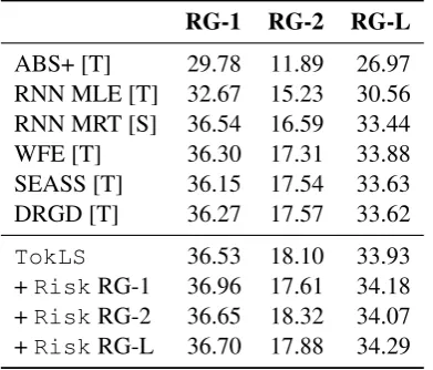
Table 6: Accuracy on Gigaword abstractive sum-marization in terms of F-measure Rouge-1 (RG-1), Rouge-2 (RG-2), and Rouge-L (RG-L) for token-level label smoothing, andRisk optimization of all three ROUGE F1 metrics. [T] indicates a token-level ob-jective and [S] indicates a sequence level obob-jectives. ABS+ refers to Rush et al. (2015), RNN MLE/MRT (Ayana et al.,2016), WFE (Suzuki and Nagata,2017), SEASS (Zhou et al.,2017), DRGD (Li et al.,2017).
with Adam (Kingma and Ba,2014) for another 10 epochs with learning rate 0.00003 and 16
candi-date sequences per training example. We conduct experiments withRisksince it performed best in trial experiments.
Different from other sequence-level experi-ments (§5), we rescale the BLEU scores in each candidate set by the difference between the maxi-mum and minimaxi-mum scores of each sentence. This avoids short sentences dominating the sequence updates, since candidate sets for short sentences have a wider range of BLEU scores compared to longer sentences; a similar rescaling was used by Bahdanau et al.(2016).
Table 5 shows the results from Wiseman and Rush(2016) for their token-level likelihood base-line (MLE), best beam search optimization results (BSO), as well as our reimplemented baseline. Risk significantly improves BLEU compared to our baseline at +2.75 BLEU, which is slightly bet-ter than the +2.33 BLEU improvement reported for Beam Search Optimization (cf.Wiseman and Rush(2016)). This shows that classical objectives for structured prediction are still very competitive.
6.7 WMT’14 English-French results
Next, we experiment on the much larger WMT’14 English-French task using the same model setup as Gehring et al.(2017b). WeTokLSfor 15 epochs
valid test
TokLS 34.06 40.58
+Risk 34.20 40.95
TokLS+ selfatt 34.24 41.02 + in domain 34.51 41.26
+Risk 34.30 41.22
[image:8.595.85.281.63.230.2]+Riskin domain 34.50 41.47
Table 7: Test and valid BLEU on WMT’14 English-French with and without decoder self-attention.
and then switch to sequence-level training for an-other epoch. Table 7 shows that sequence-level training can improve an already very strong model by another +0.37 BLEU. Next, we improve the baseline by adding self-attention (Paulus et al., 2017;Vaswani et al.,2017) to the decoder network (TokLS+ selfatt) which results in a smaller gain of +0.2 BLEU byRisk. If we trainRiskonly on the news-commentary portion of the training data, then we achieve state of the art accuracy on this dataset of 41.5 BLEU (Xia et al.,2017).
6.8 Abstractive Summarization
Our final experiment evaluates sequence-level training on Gigaword headline summarization. There has been much prior art on this dataset orig-inally introduced by Rush et al. (2015) who ex-periment with a feed-forward network (ABS+). Ayana et al. (2016) report a likelihood baseline (RNN MLE) and also experiment with risk train-ing (RNN MRT). Different to their setup we did not find a softmax temperature to be beneficial, and we use beam search instead of sampling to obtain the candidate set (cf.§6.5).Suzuki and Na-gata(2017) improve over an MLE RNN baseline by limiting generation of repeated phrases. Zhou et al.(2017) also consider an MLE RNN baseline and add an additional gating mechanism for the encoder. Li et al. (2017) equip the decoder of a similar network with additional latent variables to accommodate the uncertainty of this task.
[image:8.595.332.500.63.175.2](36.59 Riskonly vs. 36.67 Weighted), RG-2 (17.34 vs. 18.05), and RG-L (33.66 vs. 33.98).
7 Conclusion
We present a comprehensive comparison of classi-cal losses for structured prediction and apply them to a strong neural sequence to sequence model. We found that combining sequence-level and token-level losses is necessary to perform best, and so is training on candidates decoded with the current model.
We show that sequence-level training improves state-of-the-art baselines both for IWSLT’14 German-English translation and Gigaword ab-stractive sentence summarization. Structured pre-diction losses are very competitive to recent work on reinforcement or beam optimization. Classical expected risk can slightly outperform beam search optimization (Wiseman and Rush,2016) in a like-for-like setup. Future work may investigate better use of already generated candidates since invok-ing generation for each batch slows down traininvok-ing by a large factor, e.g., mixing with fresh and older candidates inspired by MERT (Och,2003).
References
Ayana, Shiqi Shen, Yu Zhao, Zhiyuan Liu, Maosong Sun, et al. 2016. Neural headline generation with sentence-wise optimization. arXiv preprint arXiv:1604.01904.
Dzmitry Bahdanau, Philemon Brakel, Kelvin Xu, Anirudh Goyal, Ryan Lowe, Joelle Pineau, Aaron Courville, and Yoshua Bengio. 2016. An Actor-Critic Algorithm for Sequence Prediction. InarXiv preprint arXiv:1607.07086.
Dzmitry Bahdanau, Kyunghyun Cho, and Yoshua Ben-gio. 2014. Neural machine translation by jointly learning to align and translate. arXiv preprint arXiv:1409.0473.
Mauro Cettolo, Jan Niehues, Sebastian St¨uker, Luisa Bentivogli, and Marcello Federico. 2014. Report on the 11th IWSLT evaluation campaign. InProc. of IWSLT.
Samidh Chatterjee and Nicola Cancedda. 2010. Mini-mum error rate training by sampling the translation lattice.
Yann N. Dauphin, Angela Fan, Michael Auli, and David Grangier. 2017. Language Modeling with Gated Convolutional Networks. InProc. of ICML.
John Duchi, Elad Hazan, and Yoram Singer. 2011. Adaptive subgradient methods for online learning
and stochastic optimization. Journal of Machine Learning Research12(Jul):2121–2159.
Jonas Gehring, Michael Auli, David Grangier, and Yann N Dauphin. 2017a. A Convolutional Encoder Model for Neural Machine Translation. InProc. of ACL.
Jonas Gehring, Michael Auli, David Grangier, Denis Yarats, and Yann N. Dauphin. 2017b. Convolutional Sequence to Sequence Learning. InProc. of ICML.
Kevin Gimpel and Noah Smith. 2010. Softmax-margin crfs: Training log-linear models with cost functions. InProc. of ACL.
David Graff, Junbo Kong, Ke Chen, and Kazuaki Maeda. 2003. English gigaword. Linguistic Data Consortium, Philadelphia.
Spence Green, Daniel Cer, and Christopher Manning. 2014. An Empirical Comparison of Features and Tuning for Phrase-based Machine Translation. In
Proc. of WMT. Association for Computational Lin-guistics.
Ralf Herbrich, Thore Graepel, and Klaus Obermayer. 1999. Support vector learning for ordinal regression .
Po-Sen Huang, Chong Wang, Dengyong Zhou, and Li Deng. 2017. Neural Phrase-based Machine Translation. InarXiv preprint arXiv:1706.05565.
Diederik P. Kingma and Jimmy Ba. 2014. Adam: A Method for Stochastic Optimization. Proc. of ICLR
.
Piji Li, Wai Lam, Lidong Bing, and Zihao Wang. 2017. Deep recurrent generative decoder for abstractive text summarization. arXiv.
Chin-Yew Lin. 2004. Rouge: A package for automatic evaluation of summaries. In Text Summarization Branches Out: Proceedings of the ACL-04 Work-shop.
Chin-Yew Lin and Franz Josef Och. 2004. Orange: a method for evaluating automatic evaluation metrics for machine translation. InProc. of COLING.
Minh-Thang Luong, Hieu Pham, and Christopher D Manning. 2015. Effective approaches to attention-based neural machine translation. In Proc. of EMNLP.
Franz Josef Och. 2003. Minimum Error Rate Training in Statistical Machine Translation. Sapporo, Japan, pages 160–167.
Romain Paulus, Caiming Xiong, and Richard Socher. 2017. A deep reinforced model for abstractive sum-marization.arXiv preprint arXiv:1705.04304. Gabriel Pereyra, George Tucker, Jan Chorowski,
Lukasz Kaiser, and Geoffrey E. Hinton. 2017. Reg-ularizing neural networks by penalizing confident output distributions. InProc. of ICLR Workshop. Marc’Aurelio Ranzato, Sumit Chopra, Michael Auli,
and Wojciech Zaremba. 2015. Sequence level Train-ing with Recurrent Neural Networks. In Proc. of ICLR.
Antti-Veikko I Rosti, Bing Zhang, Spyros Matsoukas, and Richard Schwartz. 2010. BBN System De-scription for WMT10 System Combination Task. In
Proc. of WMT. Association for Computational Lin-guistics, pages 321–326.
Alexander M Rush, Sumit Chopra, and Jason Weston. 2015. A neural attention model for abstractive sen-tence summarization. InProc. of EMNLP.
Tim Salimans and Diederik P Kingma. 2016. Weight normalization: A simple reparameterization to ac-celerate training of deep neural networks. arXiv preprint arXiv:1602.07868.
Rico Sennrich, Barry Haddow, and Alexandra Birch. 2016. Neural Machine Translation of Rare Words with Subword Units. InProc. of ACL.
Shiqi Shen, Yong Cheng, Zhongjun He, Wei He, Hua Wu, Maosong Sun, and Yang Liu. 2016. Minimum Risk Training for Neural Machine Translation. In
Proc. of ACL.
David A. Smith and Jason Eisner. 2006. Minimum Risk Annealing for Training Log-Linear Models. In
Proc. of ACL.
Nitish Srivastava, Geoffrey E. Hinton, Alex Krizhevsky, Ilya Sutskever, and Ruslan Salakhutdi-nov. 2014. Dropout: a simple way to prevent Neural Networks from overfitting. JMLR15:1929–1958. Ilya Sutskever, James Martens, George E. Dahl, and
Geoffrey E. Hinton. 2013. On the importance of initialization and momentum in deep learning. In
ICML.
Ilya Sutskever, Oriol Vinyals, and Quoc V Le. 2014. Sequence to Sequence Learning with Neural Net-works. InProc. of NIPS. pages 3104–3112.
Jun Suzuki and Masaaki Nagata. 2017. Cutting-off re-dundant repeating generations for neural abstractive summarization.arXiv preprint arXiv:1701.00138.
Christian Szegedy, Vincent Vanhoucke, Sergey Ioffe, Jonathon Shlens, and Zbigniew Wojna. 2015. Re-thinking the inception architecture for computer vi-sion.arXiv.
Ben Taskar, Carlos Guestrin, and Daphne Koller. 2003. Max-margin markov networks. InNIPS.
Ioannis Tsochantaridis, Thorsten Joachims, Thomas Hofmann, and Yasemin Altun. 2005. Large margin methods for structured and interdependent output variables. Journal of Machine Learning Research
6:1453—-1484.
Ashish Vaswani, Noam Shazeer, Niki Parmar, Jakob Uszkoreit, Llion Jones, Aidan N. Gomez, Lukasz Kaiser, and Illia Polosukhin. 2017. Attention is all you need. arXiv.
R. J. Williams. 1992. Simple statistical gradient-following algorithms for connectionist reinforce-ment learning. Machine Learning8:229—-256. Sam Wiseman and Alexander M. Rush. 2016.
Sequence-to-sequence learning as beam-search op-timization. InProc. of ACL.
Yonghui Wu, Mike Schuster, Zhifeng Chen, Quoc V Le, Mohammad Norouzi, Wolfgang Macherey, Maxim Krikun, Yuan Cao, Qin Gao, Klaus Macherey, et al. 2016. Google’s Neural Machine Translation System: Bridging the Gap between Human and Machine Translation. arXiv preprint arXiv:1609.08144.
Yingce Xia, Fei Tian, Lijun Wu, Jianxin Lin, Tao Qin, Nenghai Yu, and Tie-Yan Liu. 2017. Deliberation networks: Sequence generation beyond one-pass de-coding. InProc. of NIPS.