MASTER THESIS
EVALUATING THE
BEHAVIOR OF EMBEDDED
CONTROL SOFTWARE
using a Modular Software-In-The-Loop
Simulation Environment and a Domain Specific
Modeling Language for Plant Modeling
Christian Terwellen
FACULTY OF ELECTRICAL ENGINEERING, MATHEMATICS AND COMPUTER SCIENCE
SOFTWARE ENGINEERING (SE)
EXAMINATION COMMITTEE
Abstract
During the development of high performance mechatronic systems it is necessary to ensure high quality products and short time-to-market. Because the Embedded Software (ESW) is a fundamental part of such systems, it is necessary to provide a well suited testing environment. A challenge in testing ESW is that its hardware environment, called the plant, is needed to properly evaluate its behavior. It is, in many cases, not feasible to test the ESW on the hardware because there are no, or not enough, hardware resources available. To address this problem, the ESW can be tested using a software simulation of the plant behavior. This leads to several advantages. For example, the plant hardware is not needed for testing the ESW and it is possible to test faster, more frequent and more effective.
Since five years, such a simulation environment has been in use at Oc´e to test the part of the ESW that controls the paper transport inside the printer. This is done by executing the ESW together with a plant model, emulating the hardware included in the paper transport, on a software engineer’s workstation. Due to the great success of this simulation environment, the goal of this project is to extend the simulation environment to be able to test the ESW of the whole printer, using simulated plant models.
In order to achieve this goal, the architecture of the simulation environment has been reviewed and newly designed to meet the new requirements. The new version of the simulation environment is well prepared for the future use of multiple different plant models, which is important to reach the goal of testing all printer functions in the simulation environment.
To support the creation of plant models, a plant modeling framework has been developed. This plant modeling framework enables short modeling times and re-quires only little domain knowledge of the plant concepts and the modeling of physical systems. These are important properties of the framework, since the main users of the framework are software engineers.
I dedicate this thesis to Annika and my family,
Acknowledgments
I would like to express my sincere thanks to my supervisors. Dr. Ir. Lodewijk Bergmans, I would like to thank for his outstanding support throughout the project. With his guidance and constructive criticism he contributed tremendously to the success of my project. I also would like to thank Dr. Lou Somers for the technical discussions, which guided me through the different stages of my project. Without his detailed knowledge of the field of high performance printing systems, the project would not have been possible. I would like to express my gratitude towards all my supervisors, Dr. Ir. Lodewijk Bergmans, Dr. Lou Somers and Dr. Ing. Christoph Bockisch for their invaluable assistance, support and guidance during the writing of this thesis. Besides, I would like to thank Oc´e for providing me with the opportunity to carry out my final project in such an interesting field of research.
Special thanks also to Henri Hunnekens and Ben van Rens for supporting me during the redesign of the architecture of SIL. Their experience with the simulation environment and their immediate feedback on the different design stages contributed immensely to the results of the redesign of the SIL simulation environment. Besides, I would like to thank Ruud Jackobs and Harald Schwindt for their outstanding support during the design of EZ-VirtualPrinter. I also would like to express my gratitude to Chidi Okwudire, who redesigned MoBasE during the time I carried out my final project. In many meetings we discussed and found the right way to add the information needed in this project to MoBase. The support received from all the colleagues at Oc´e, who contributed to this project and are not named explicitly, was vital for the success of the project.
Contents
1 Introduction 1
2 Project Context 3
2.1 Problem Statement . . . 3
2.2 Motivation for the Initial SIL Simulation Design . . . 4
2.2.1 Traditional Development Process of Mechatronic Systems . . . 4
2.2.2 Drawbacks Regarding Testing Performance . . . 5
2.2.3 Advantages of Testing ESW in a Simulation Environment . . . 5
2.2.4 The Predecessors of SIL . . . 5
2.2.5 Goals of the Initial SIL Implementation . . . 8
2.3 Current Situation of SIL . . . 8
2.3.1 The Software under Test (SuT) . . . 8
2.3.2 Global Structure of SIL . . . 11
2.3.3 Interface between SIL, SheetLogic and ESW . . . 15
2.3.4 Running a Simulation . . . 16
3 Refining the Architecture of SIL 17 3.1 Requirements for SILv2 . . . 17
3.1.1 Requirements . . . 17
3.1.2 Key Drivers . . . 17
3.2 Detailed Analysis of Problems in SILv1 . . . 18
3.2.1 Communication of ESW and SheetLogic . . . 18
3.2.2 SheetLogic as the Central Concept of Simulating Plant Behavior . . . 19
3.3 Design Decisions . . . 19
3.3.1 Generic or Specific Interface . . . 20
3.3.2 Storage and Communication of Communication Variables . . . 21
3.3.3 SheetLogic and the Low Level Control . . . 24
3.4 New Communication Strategy . . . 25
3.4.1 Global Principle . . . 25
3.4.2 Changed and added Entities of SIL . . . 29
3.5 Evaluation . . . 31
3.5.1 Change Case Impact Analysis . . . 31
3.5.2 Key Drivers . . . 36
3.5.3 Meeting Requirements . . . 38
3.5.4 Additional Advantages of SILv2 . . . 39
3.6 Implementation . . . 39
3.6.1 I/O-layer . . . 40
3.6.2 SIL Core . . . 42
3.7 Conclusion . . . 50
4 The SILv2 Plant Modeling Framework 51 4.1 Requirement Analysis . . . 51
4.1.1 Stakeholders . . . 51
4.1.2 Requirements . . . 52
4.2 Design Decisions . . . 53
4.2.1 Level of Abstraction . . . 53
4.2.2 (C)OTS vs. Custom-Made . . . 54
4.2.3 Modeling by Hand and Generation of Plant Models . . . 55
4.2.4 Implementation Environment/Tools for Implementing the DSML Tools . 56 4.2.5 Including the SIL Interface . . . 58
4.3 The Custom-Made High-Level Plant DSML Approach EZ-VirtualPrinter(EZ-VP) 60 4.3.1 Example Printer Models . . . 60
4.3.2 Identification of Overlapping Concepts . . . 60
4.3.3 Controlling the Plant . . . 62
4.3.4 Abstracting the Plant Concept of Moving Elements . . . 63
4.3.5 Abstracting the Plant Concept of Transport of Material through the Printer 69 4.3.6 The Whole Meta Model . . . 77
4.3.7 Tools of EZ-VP . . . 78
4.4 Matlab Simulink SIL Plant Model Simulation Modules . . . 80
4.5 Implementation . . . 81
4.5.1 EZ-VP-Edit . . . 82
4.5.2 EZ-VP Back-End . . . 86
4.5.3 Matlab Simulink Plant Model Simulation Module Creation for SIL . . . . 88
4.6 Case Studies . . . 90
4.6.1 Case Study 1. Moving Elements . . . 90
4.6.2 Case Study 2. Material Transport . . . 94
4.7 Evaluation . . . 97
4.8 Conclusion . . . 99
5 Discussion and Future Work 100
6 Conclusion 102
A I/O-layer 106
List of Figures
1.1 The VarioPrint 6250. . . 1
2.1 The interdisciplinary development process of high performance printers. . . 4
2.2 An example of the internals of a printing system. . . 6
2.3 A paper path layout. . . 6
2.4 A simulation environment for testing the paper path software in Matlab Simulink. 7 2.5 Architecture of the embedded control software when in SIL Simulation. . . 9
2.6 The simulated CAN bus. . . 10
2.7 Architecture of the embedded control software. . . 10
2.8 I/O-layer macros and the use of them. . . 11
2.9 The current structure of the simulation environment. . . 12
2.10 The Argus visualization tool. . . 13
2.11 The RemoteControl. . . 14
2.12 The current interface during startup and while running. . . 15
2.13 Plotting I/O-device values while simulating. . . 16
3.1 Low level control in SILv1. . . 19
3.2 Storing variables only in the SIL core. . . 21
3.3 Storing variables only in one simulation module. . . 22
3.4 Storing variables in the SIL core and a copy in the simulation modules. . . 22
3.5 Low level control in SILv2. . . 25
3.6 The structure of the SIL interface structure. . . 26
3.7 The new interface between simulation modules and the SIL core during initial-ization. . . 27
3.8 The new interface between simulation modules and the SIL core when running. 28 3.9 The global structure of SILv2. . . 28
3.10 The entities changed in this project (everything that is solid black). . . 29
3.11 The new SIL core. . . 30
3.12 Overview of proxies in distributed simulation. . . 34
3.13 Overview of proxies in distributed simulation. . . 35
3.14 RoseRT structure diagram of the SIL core. . . 43
3.15 RoseRT state diagram of the module adapter component. . . 44
3.16 The SIL console menu to plot variables. . . 47
3.17 The glue layer to adapt the communication of SheetLogic to the new interface. . 48
3.18 The glue layer to adapt the communication of SheetLogic to the new interface. . 48
4.1 Creation of plant model simulation modules with the DSML. . . 57
4.2 Three of the four printers inspected for the domain analysis. . . 61
4.4 The carriage of an Arizona wide format printer. . . 64
4.5 Simple example system. . . 64
4.6 Part of the meta model capturing the concept of moving elements. . . 65
4.7 Instantiation of the meta model with the system of figure 4.5. . . 67
4.8 Another example system for the concept of moving elements. . . 67
4.9 Instantiation of the meta model with the system of figure 4.8. . . 68
4.10 Behavior of theM ovingElementin EZ-VP. . . 69
4.11 An example material transport system in a printer. . . 70
4.12 Meta model of the material transport concept. . . 71
4.13 Instantiation of the example material transport system from figure 4.11. . . 72
4.14 Example material transport system. . . 73
4.15 Instantiation of the example material transport system from figure 4.14. . . 74
4.16 Material transport plant model behavior. . . 75
4.17 Material transport plant model behavior. . . 76
4.18 Material transport plant model behavior. . . 76
4.19 Material transport plant model behavior. . . 77
4.20 The whole meta model, comprising the concept of moving elements and the transport of material through the printer. . . 78
4.21 Creation of plant model simulation modules with EZ-VP and Matlab Simulink. 79 4.22 EZ-VP-Edit in Eclipse. . . 80
4.23 Example Matlab Simulink model. . . 81
4.24 The EMF ecore diagram editor. . . 83
4.25 The generator model. . . 83
4.26 EZ-VP-Edit. . . 84
4.27 EZ-VP-Edit. . . 85
4.28 EZ-VP meta model implemented in RoseRT in the back-end. . . 86
4.29 Structure of the EZ-VP back-end. . . 87
4.30 The system modeled with EZ-VP in this case study. . . 90
4.31 The system modeled with EZ-VP in this case study. . . 90
4.32 Running the System with control software in SIL. . . 92
4.33 Running the System with control software in SIL. . . 92
4.34 Running the System with control software in SIL. . . 93
4.35 Running the System with control software in SIL. . . 93
4.36 Running the System with control software in SIL. . . 94
4.37 An example material transport system in a printer. . . 94
4.38 The system modeled with EZ-VP in this case study. . . 95
4.39 Running the System with control software in SIL. . . 96
4.40 Running the System with control software in SIL. . . 96
List of Tables
Listings
3.1 The SIL interface structure. . . 40
3.2 Part of the macro for simple sensors. . . 41
3.3 The function addInpComponent. . . 41
3.4 The whole simple sensor I/O macro. . . 41
3.5 Get variables handles. . . 43
3.6 Tick transition of the ModuleAdapter. . . 44
3.7 f UpdateValues() . . . 44
3.8 f WriteValues() . . . 44
3.9 getVariableHandle() . . . 45
3.10 setValues() . . . 46
3.11 getValues() . . . 46
3.12 updateActuators() . . . 49
4.1 The model stored in XML. . . 79
4.2 The created model in XML. . . 85
4.3 Adding variables to the SIL interface structure when an I/O-device is created. . . 87
4.4 Adding variables to the SIL interface structure. . . 89
4.5 void sil GetInterface() in the custom code block. . . 89
4.6 void sil StartScheduling() in the custom code block. . . 89
4.7 Control software for the moving element. . . 91
4.8 Init of the control software for the material transport. . . 95
4.9 Control software for the material transport. . . 95
A.1 changed parts of ln iolayerTargetMacros.c . . . 106
Glossary
RoseRT IBM Rational Rose RealTime, A development and code-generation en-vironment for the development of real-time software.
ESW Embedded Software, The software that is developed and deployed on embedded controllers to control the behavior of Mechatronic Systems.
Mechatronic System
System consisting of subsystems from different domains, like Mechanics, Electronics, hydraulics, pneumatics and software engineering.
SIL Software-In-The-Loop, When using a SIL simulation, the ESW is exe-cuted with a model of the plant. SIL is also the internal name of the SIL simulation environment used within Oc´e.
Named Pipe Named Pipe or also called FIFO for first in first out is a kind of inter process communication.
CAN bus The controller area network (CAN) bus, designed by Bosch, is a standard designed for the communication between micro controllers in vehicles. The standard is also used in other applications for communication means between micro controllers.
Main node Supervisory control that controls several sub nodes
Sub node Controller that controls I/O-devices and is controlled by a main node.
Paper handling The handling of sheets as they move through the printer. That com-prises accelerating and decelerating sheets according to a timing model, correction of the sheet position on the Z axis, as well as the correction of askew papers (rotation on Y axis)
SheetLogic SheetLogic is the name of the paper path plant model used in the SIL simulation environment.
DLL A DLL (Dynamic Link Library) is a library of functions, which can be used by multiple computer programs. A DLL can be loaded and used dynamically in runtime.
Simulation Module
The term simulation module is used to describe plant models or ESW that are compiled to a DLL and can be loaded and executed by SIL. Plant model module and ESW module are also used if a separation is needed between the two types.
Chapter 1
Introduction
Oc´e is a company that offers office printing and copying systems, high speed digital production printers and wide format printing systems for both, technical documentation and color display graphics as well as related software. It was founded in 1877, with headquarters in Venlo, The Netherlands. Oc´e is active in over 100 countries and employs some 20,000 people worldwide. Total revenues in financial 2010 amounted to approximately 2.7 billion. The main Research and Development site is also located in Venlo, The Netherlands. This department develops new printers including mechanics, electronics and embedded control software.
To give an impression of a high volume, high performance printer, figure 1.1 shows a Vari-oPrint 6250. The printer consists of Paper input modules (PIM) on the left, the Print Engine
Figure 1.1: The VarioPrint 6250.
(PE) and finisher (FIN) modules on the right. The printer is suitable for from 600,000 up to 8,000,000 prints per month and has a print speed of 250 A4/letter prints per minute or 132 A3 prints per minute. The printer can be equipped with up to 12 input trays, which can be refilled during printing and can hold different types of paper (size, coating). The output storage can take on 6000 prints but prints can be unloaded while printing. The toner can also be refilled while printing.
Even if there is hardware available, it is often not feasible to let every software engineer test the written software on a prototype. Testing on the target hardware can also be ineffective due to long preparation and the fact that error injection and reproduction is difficult. In the case of high performance mechatronic systems it is also likely that the needed hardware is expensive.
To provide a more efficient way of testing, Oc´e has developed a Software-in-the-loop (SIL) simulation environment (internally simply called SIL), which allows to test the software on an ordinary workstation. In this environment, the ESW is executed with a model of the plant that emulates the behavior of the real plant. Originally, SIL was only used to evaluate the ESW that does the paper handling. The paper handling is the control of the flow of paper through the printer (paper transport) along the so called paper path. Van der Hoest [13] established the foundation of the SIL simulation environment in 2006. After that other works in this context have been performed to add new features or improve the simulation environment. Examples are the simulation of the print process in laser printers [7] or an interactive visualization [8]. Not all those improvements are used in the current SIL simulation environment because some are specific to one kind of printer architecture, and can therefore not be used in all development projects.
The goal of this project is to extend the current SIL simulation framework in a generic way to make modeling and simulation of the behavior of the remaining plant elements of a printer possible. The extension of SIL and the modeling framework, presented in this document, offer several advantages in different stages of the development process. It makes it possible to test more frequent, more controlled and on the developer’s workstation and therefore provides shorter feedback cycles during software development. It is also possible to test the software before the actual hardware is build. Those advantages should ultimately lead to a shorter time to market and better quality.
Previous to this work a survey on plant modeling approaches [12] has been created to get a broad overview of different techniques that can be used to model physical systems. The paper also provides a taxonomy for plant modeling approaches to make a clear categorization possible. After the survey part, the paper presents and discusses ways to structure and modularize plant models to enhance maintainability and extensibility.
Chapter 2
Project Context
This section presents the context in which this project is carried out. The first section of this chapter presents the goals for the evolution of SIL and the research questions identified for this project. After that motivations and the problem statement that lead to the initial design of a SIL simulation environment are presented. Last, the current situation of SIL is described.
2.1
Problem Statement
SIL is widely use in several projects to test the embedded software for the paper handling. Several projects use SIL for the major part of the testing work, when developing the ESW of a new printer. Since SIL is used for testing the ESW with great success, there are new goals for the evolution of SIL or the use of simulation in the development process in general. The long term vision is that in the future a virtual printer environment is used to develop new printers. This environment consists of models of different parts of the printer from different domains. This environment is used to test the system even before the first mechanical prototype is built. The following advantages have been identified for the use of such a virtual printer system.
• Critical interactions between disciplines can be studied by combining models of the indi-vidual aspects. This fits in a multi-disciplinary Model-Driven-Design approach.
• A virtual printer has the advantage of lower price and shorter lead and adaptation time.
• When the first physical prototype is built, many issues are already solved.
• The virtual printer gives more control over the test conditions (such as climate, error conditions, and tolerances)
• During the development, knowledge is gathered in models, which are used for simulation but also as documentation.
• Better quality due to regression testing.
• A virtual printer consumes less energy and paper.
The short term goal for SIL is to create a virtual version of the whole printer, which is only used to evaluate the ESW and not systems from other disciplines (mechanics, electronics). In this environment software engineers can compose a test system out of ESW modules and plant model modules. All parts of the printer can be easily modeled and used as plant model modules for simulation in SIL. SIL provides easy deployment, resulting in high acceptance and it is part of an integrated tool chain, used in product development.
Two research questions can be identified that summarize the problems to be solved in order to achieve the short term goals.
• How to design a plant modeling framework for the creation of plant models for simulation
in a Software-In-The-Loop simulation environment that is expressive enough to model a multitude of domain concepts of high performance printers, but also uses an adequate level of abstraction to make the approach usable for non-domain experts?
• How to develop a modular and extensible Software-In-The-Loop simulation environment
that enables the execution of multiple embedded software modules and multiple plant models with the goal of evaluating the behavior of the embedded software?
These two questions are addressed in the following two chapters. Chapter 3 describes the design and implementation of a modified and extended SIL. Chapter 4 presents the developed of a plant modeling approach.
2.2
Motivation for the Initial SIL Simulation Design
This section illustrates the motivations for the initial development of SIL. For this project, the documentation of earlier SIL related projects has been examined to get a clear view on motivations, requirements and use cases that has been identified in those projects.
2.2.1 Traditional Development Process of Mechatronic Systems
To better understand the motivations for the initial development of SIL, this section describes the common traditional development process for the development of mechatronic systems. Sev-eral steps are performed leading from the concept to a finished product. Figure 2.1 shows the development time of the involved domains in the traditional process of a project.
Figure 2.1: The interdisciplinary development process of high performance printers.
design is further developed by mechanical engineers. At a certain stage electrical engineering becomes more involved in the process. After some time software engineers begin to develop the corresponding ESW for the printer model. While developing the ESW, it is important to continuously test the ESW with the plant to evaluate its behavior. In early states those tests are executed on hardware test boards that contain the I/O hardware that is going to be used. Those test are done to test the low level control of sensors and actuators rather than the high level logic of ESW. In later stages several prototypes so called lab models are built. These lab models are used to prove that the designed concept works and can be used for testing the high level logic of the ESW. The result of the development is a so called engineering prototype, which is given to the manufacturing department where it is further optimized in terms of ease-of-use, print quality and speed.
Important factors in the development process are:
• Short time-to-market: The time it takes from initial concept to product.
• High printer performance: Such as energy consumption, print speed and print quality.
• High printer reliability: Achieving high quality of hard- and software to increase the mean time between failures.
A problem that can be identified in this development process is that embedded software can be developed from the beginning, but that it can not be tested till the corresponding hardware is created. Thus, the development of the ESW dependents on the progress of the other engineering disciplines. This leads to the situation that the ESW can not be tested in early stages of a project when there is not yet a prototype available.
2.2.2 Drawbacks Regarding Testing Performance
Even if there is hardware available, it is often not feasible to let every software engineer test the written software on a prototype. Testing on the target hardware can also be ineffective due to long preparation and the fact that error injection and reproduction is difficult. In the case of high performance mechatronic systems it is also likely that the needed hardware is expensive.
2.2.3 Advantages of Testing ESW in a Simulation Environment
So, a testing environment, which could be used to test the ESW without the hardware plant would lead to several advantages. A possible approach to solve the above mentioned problems is to model and simulate the behavior of the plant of the target mechatronic system in software. That enables the software engineer to carry out tests in a simulated instead of the real environ-ment. An advantage is that the software can be tested on the software engineer’s local system and therefore allow shorter feedback cycles. It is further possible to create and investigate situ-ations that are difficult or not even possible to create and investigate when testing with the real hardware though it is relevant to test them. Another major advantage is that regression testing is possible. So, simulation based testing is likely to improve two of the three important factors identified for the development process of mechatronic systems in section 2.2.1, namely “Short time-to-market” and “High printer reliability”. The “time-to-market” gets shorter because the development of the ESW can start earlier. The ESW is likely to have a higher reliability because it is tested more frequently (regression testing).
2.2.4 The Predecessors of SIL
in the development of ESW for the paper path. The following subsection provides background information about the paper handling of a printer.
Paper Handling
The paper path describes the path of the paper as it moves through the printer. Figure 2.2 shows an example of a printer’s internals. The figure shows the way of the paper from the paper input
Figure 2.2: An example of the internals of a printing system.
[image:18.595.141.452.169.396.2]module through the print engine to the finisher, which, in this case, stacks the printed paper. Most printers can have multiple configurations. That means different numbers of PIMs and different numbers and/or types of finishers. In addition, some printers have different versions that differ in speed. Figure 2.3 shows a 2D sketch of an example paper path.
Figure 2.3: A paper path layout.
which move the paper. Sensors are used to sense the presence or absence of paper. During the design of the physical (mechanical) paper path of a printer, a timing model is created that describes the desired movement of the sheets as a speed profile. So it is defined for the sheet at which point on the paper path it has which speed. In the printer this model is implemented by the use of pinches that are accelerating or decelerating the sheets. All pinches in between such pinches, which accelerate or decelerate a sheet, run at a constant speed. For example, a sheet enters the paper path, described in figure 2.3, with a speed of 1,5 m/s. P0 andP1 run at a constant speed so that the paper is further transported with 1,5 m/s. After the paper leaves
P1 and is only in contact with P3, P3 decelerates the paper to 0,9 m/s. P4 again runs at a constant speed so that the paper is transported further with 0,9 m/s. The timing model is used as an input for the ESW, which uses the timing information to control the involved motors in such a way that the accelerations and decelerations are performed. Next to the variation in speed, there are different kinds of checks and corrections of the sheet positions in z-position and to correct occurring rotation of the sheets, as the sheets travel through the printer.
There are several reasons why the development of the paper handling can be difficult.
• Sheets can have different formats.
• Print jobs can contain sheets that are printed simplex (1-sided) and/or duplex (2-sided).
• Some printers support different throughput rates, for example, both 50 and 70 pages per minute.
• During development the paper path typically changes with each new prototype, which leads to repeated redefinition of the timing model.
• When the image is printed on a sheet, it is important that the sheets position is aligned with the image.
The Matlab Simulink Paper Path Simulation
Figure 2.4: A simulation environment for testing the paper path software in Matlab Simulink.
Figure 2.4 shows the high level structure of the simulation environment. The blockSheetLogic
This simulation was evaluated by different software engineers and was considered very help-ful in the process of developing ESW. Van der Hoest identified two major drawbacks of this simulation environment, maintainability and license cost [13]. It is hard to maintain the Sheet-Logic Matlab Simulink block because for doing this one needs to be able to model a physical system in Matlab Simulink. In this case the hardware of the paper path of a printer has to be modeled accurate enough to use the model for evaluating the ESW. This is not feasible because Matlab Simulink is not widely used by the software engineers, which would have to perform this task. Using Matlab Simulink as a simulation environment would also lead to high license cost because a Matlab Simulink license is needed for every software engineer that uses this tooling.
2.2.5 Goals of the Initial SIL Implementation
After identifying flaws in the classical way of testing ESW in the context of a multidisciplinary project and recognizing possibilities and advantages of a simulation based testing approach, the initial SIL was implemented with the following key drivers [13]:
• Ease-of-use. SIL should be easy to use for software engineers and integrators to be accepted by them. This is especially the case for the process of specifying a printer layout and preparing the ESW for simulation.
• Maintainability. Especially for the modeled plant behavior.
• Early feedback. Simulating and testing should provide immediate feedback.
• Reliability. The simulation should be accurate and reproducible. When a certain test case fails, it should be possible to repeat the simulation with exactly the same results, for further analysis.
• Low cost. The use of commercial products that cause high license costs should be avoided.
2.3
Current Situation of SIL
This section presents the initial SIL implementation to give a technical context for this project. The SIL simulation tooling has undergone several extensions and improvements since the first release in 2006. SIL and also the corresponding visualization tool, Argus, where attractive fields of research in several research projects that were carried out by students.
First an overview of the architecture of the software under test is given. After that the structure of SIL and the interfacing with the ESW and the plant models are presented.
2.3.1 The Software under Test (SuT)
The architecture of the ESW and the needed steps to prepare the ESW for execution in the SIL environment, are a major concern because the software should not be changed for the purpose of testing.
Software Architecture
provides functions to communicate with different I/O-devices. Sub nodes have a time sliced structure. That means that a function that initiates all calculations and controls, is called in a defined frequency by the real-time embedded system. This function is called “tick” function. Figure 2.5 shows the high level architecture of the embedded software of most printers. Main
Figure 2.5: Architecture of the embedded control software when in SIL Simulation.
and sub nodes are implemented using C/C++ in RoseRT. The controller software is split up in different parts, which are implemented using different general purpose and scripting languages. The main node communicates with the sub nodes via a CAN bus. The communication between controller and main node is realized using an interface based on high-level commands. For some I/O-devices an additional low level control layer is used, next to the I/O-layer, that implements low level control functionality. This layer is often implemented using FPGAs. This is, for example, used for stepper motor control. If the ESW starts a stepper motor, the I/O-layer calls a function of the low level control that starts the motor at a certain time or position with a certain speed etc. The low level control translates this function call into a low level signal that is send to the stepper motor.
Preparing the ESW for SIL Simulation
Figure 2.6: The simulated CAN bus.
In the normal case, when the ESW is compiled for an embedded system, an I/O-layer is used to implement the low level communication with I/O-devices or the low level control. For different target embedded systems, different I/O-layers are available. When the ESW is build for SIL, a SIL simulation I/O-layer is used. The interface between the ESW-layer and the I/O-layer stays the same. An overview of the architecture of a sub-node for a target embedded system and for simulation is shown in figure 2.7. The communication between the SIL simulation I/O-layer is based on high-level sensor and actuator signals. Examples for those signals are the logical value of a digital actuator or sensor (ON or OFF) or the “start at time” or “start at position” command of a stepper motor. When the ESW is run and tested in the SIL simulation, it is
Figure 2.7: Architecture of the embedded control software.
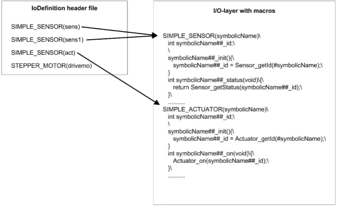
in SIL. Figure 2.8 shows the concept of the I/O-layer. The different I/O-elements are specified in an I/O-specification header file (left). This file is a list of I/O-devices, that uses macros to specify each I/O-device. These macros (right) are used to create functions, which can be used by the ESW to communicate with I/O-devices. So, every definition in the ESW header creates functions specific for this device function names based on the name of the device. Which functions are generated depends on the type of I/O-device and therefore which macro is used.
Figure 2.8: I/O-layer macros and the use of them.
2.3.2 Global Structure of SIL
The global structure of SIL did not change significant over the time SIL was used. The structure has been examined in the beginning of this project to be able to evaluate its suitability for the intended extensions. Figure 2.9 shows the different entities of SIL. Subsequently, all entities are described in short.
SIL core and SheetLogic
The SIL simulation environment is a custom made tool implemented in RoseRT using C/C++. In the current SIL simulation environment, the most important plant model that is used, is a model of the paper path of the printer, called SheetLogic. SheetLogic consists of different I/O-devices and mechanical parts that are simulated to emulate the paper path behavior. Examples of those elements are motors, stepper motors, pinches, pinch lift actuators, or paper path segments. Important to mention is that the low level control layer is also included in SheetLogic. SheetLogic uses these elements to create a model of the printer’s paper path by reading the specification and properties of different parts from MoBasE (described in the next subsections). It is embedded in the SIL core because SIL was initially designed to only test the ESW for the paper handling. SIL and SheetLogic are coupled because SIL needs information about the I/O-devices used in SheetLogic, to set up the connection between ESW and SheeLogic (section 2.3.3).
Figure 2.9: The current structure of the simulation environment.
of all loaded ESW modules. Since the ESW of the nodes is time sliced as discussed earlier, the clock can call the “tick” function of the ESW. SheetLogic has also a “tick” function that initiates the calculation of a new state. For SheetLogic and all ESW modules, the sample frequency can be adjusted. While running, the clock calls the “tick” function of all modules and SheetLogic according to the defined schedule.
MoBasE
Visualization
The visualization front-end of SIL is called Argus. Argus provides different functionality to visualize the state of SheetLogic. The properties of the different parts (pinches, sensors, etc) can be visualized as a list or in a 3D environment. The 3D animation shows the paper path of the tested printer, consisting of segments, pinches, sensors and the moving sheets of paper (figure 2.10). Argus also provides functionality to manipulate the simulation by, for example, changing sensor actuator values or stopping sheets. This is done via the so called command interface.
Figure 2.10: The Argus visualization tool.
I/O-layer
The I/O-layer, as mentioned in section 2.3.1, is used to let the ESW communicate with the hardware on the target hardware environment. When the ESW is executed in SIL, the target hardware I/O-layer is replaced with a SIL simulation specific I/O-layer that translates function calls of the ESW to the I/O-layer into function calls to SheetLogic.
ESW
The block ESW contains the software that has to be tested. As described in section 2.3.1, the SuT comprises the main node as well as the sub node(s). But only the sub nodes communicate with SheetLogic via the I/O-layer. The main node in contrast, communicates with the remote control and the sub nodes.
Stub
case of the ESW. This mechanism was added to SIL as a first possibility to emulate the plant behavior of printer parts other than the paper path.
Embedded Software Logging
The ESW has extensive logging capabilities, which are used to debug the embedded software and to evaluate test cases.
Remote Control
The so called remote control is a java application that emulates the printer controller. It can, for example, be used to start print jobs and to read the machine state. The user interface of the remote control is shown in figure 2.11
Figure 2.11: The RemoteControl.
Test Executor
The test executor can be used on top of the remote control to automatically run test cases.
VirtualSystem
CommandInterface
The command interface is used to inject error into SheetLogic. It can also be used to request the state and value of sensors and actuators. This functionality can be used by the TestExecutor or the visualization.
2.3.3 Interface between SIL, SheetLogic and ESW
Since the goal of this project is to add new plant models to SIL, the interface of SIL and the ESW is reviewed. The interfacing of the ESW, respectively the I/O-layer, and SheetLogic is set up by the SIL core in the beginning of the simulation. During the initialization of the simulation,
Figure 2.12: The current interface during startup and while running.
2.3.4 Running a Simulation
When running a simulation the simulation can be controlled by the remote control, which emulates the controller of the printer. The RemoteControl application is shown in figure 2.11.
The behavior of the simulated printer and the ESW can be analyzed using Argus, ESW logging and the tooling for plotting actuator and sensor values. Argus provides different tools for visualization like a 3D visualization, list views of all I/O-devices and recording capabilities. In addition, Argus can be used to inject errors into SheetLogic. Argus is shown in figure 2.10.
Figure 2.13 shows the tool dPlot which is used to plot values of I/O-devices from SheetLogic. The SIL core is executed in a console application, which provides a simple menu to plot graphics (lower left corner in figure 2.13).
Chapter 3
Refining the Architecture of SIL
This chapter presents the design of a evolved version of SIL, which meets the requirements that are derived from the short term goals from section 2.1. For convenience the new version is referred to as SILv2 and the old as SILv1 throughout the document. The research question, discussed in this chapter is:
• How to develop a modular and extensible Software-In-The-Loop simulation environment
that enables the execution of multiple embedded software modules and multiple plant models with the goal of evaluating the behavior of the embedded software?
This chapter is organized as follows. First requirements and key drivers for the development of SILv2 are identified. After that, design decisions are discussed and the design for SILv2 is presented and evaluated. Subsequently the implementation and integration into SIL is discussed. Finally some conclusions are drawn.
3.1
Requirements for SILv2
3.1.1 Requirements
From the short term goals for the evolution of SIL (section 2.1), several functional and non-functional requirements for the evolution of SIL have been derived, as shown in table 3.1.
R1 ESW shall be encapsulated within simulation modules.
R2 Plant models shall be encapsulated within simulation modules. R3 A simulation shall be composed of multiple simulation modules.
R4 Plant models can be implemented using different plant modeling tech-nologies.
R5 Communication between ESW simulation modules and plant model sim-ulation modules shall be based on a generic and well maintainable in-terface.
Table 3.1: Requirements for SILv2.
3.1.2 Key Drivers
From the short term goals (section 2.1), it can be derived that the new SIL design should be:
• Generic. The SIL core and the communication between the SIL core and the simulation modules should be generic.
• Extensible. There are many imaginable extensions and change cases for SIL (new types of ESW or plant models). By Modularizing SIL and using generic ways of communication between the entities, SIL can adapt more easily to future changes and extensions.
• Composable. Simulation modules should be composable to make it possible to run simu-lations of sub-parts of a printer or of the whole printer.
• Efficient. SIL should have good performance so that it is possible to run the simulation in a decent speed. In the current situation, the main load is caused by the SheetLogic. This can not be changed by SILv2, but a goal is that the performance stays approximately the same compared to SILv1 (+- 5%).
3.2
Detailed Analysis of Problems in SILv1
SIL was originally designed as a dedicated test tool for testing the ESW that controls the paper path of a printer. The short term goals are that SIL evolves to a global test framework for ESW in general. So, SILv1 has been evaluated regarding the requirements and qualities to identify problems that need to be solved in order to meet the requirements. For each problem identified in this section, the related requirement or requirements from table 3.1 are given.
3.2.1 Communication of ESW and SheetLogic
The interface and communication between ESW and SheetLogic, presented in section 2.3.3, is a major concern. The current techniques introduce several problems with respect to the requirements of SILv2.
Coupling of SIL Core and SheetLogic/ other plant models
Related requirements: R1, R2, R3, R4, R5.
The SIL core sets up the connection between the ESW module and SheetLogic by transmitting function pointers, that point to functions of I/O-devices in SheetLogic, in the ESW module. That implies that these functions are known by the SIL core. That hinders the separation of SheetLogic ( or plant model simulation modules in general) and the SIL core, which is desirable for the modularization of SIL. Another problem occurs if several plant model simulation modules and several ESW modules are composed in the future. The SIL core needs information about which functions are located in which plant model simulation module and also which function pointers are required by which ESW module. This introduces strong coupling of the SIL core and the different plant model simulation modules.
Growing Interface between ESW and SheetLogic
Related requirements: R5.
3.2.2 SheetLogic as the Central Concept of Simulating Plant Behavior
Related requirements: R1, R2, R3.
In SILv1, SheetLogic is the only plant model in use (next to the stub mechanism) and can be seen as the central point of plant behavior simulation. For this reason some features are included in SheetLogic that should be part of the SIL core, when SIL supports multiple plant model simulation modules. Those features are the connection to the visualization and to the so called command interface, which is used for error injection and debugging. Even the plant behavior implemented using the stub mechanism (section 2.3.2) is heavily dependent on the implementation in SheetLogic. This is because of the fact that the I/O-devices, controlled by the stub, are located in the SheetLogic and are controlled by the stub via the same interface that is also used by the ESW (though with inverted behavior, writes sensors and reads actuators).
Another identified problem is that parts of the control software, the low level control, is included in SheetLogic, which makes the interface to some I/O-devices very complex. The interface between I/O-layer and low level control, so between the ESW simulation module and the SheetLogic, is based on function calls (figure 3.1). For a stepper motor the interface consists of 22 functions. Because of the fact that the low level control is totally integrated in SheetLogic, the interface between SIL core and simulation module has to implement those functions. It would also be a better logical separation to make the low level control part of the ESW simulation modules because it is logically part of the control.
Figure 3.1: Low level control in SILv1.
3.3
Design Decisions
3.3.1 Generic or Specific Interface
SILv1 uses an I/O-device specific interface for communication between SIL core and simulation modules. That means the communication is based on using function calls to specific simulated I/O-devices. An example is the simple sensor I/O-device, which is a digital sensor that can be in high or low state. Even for this simple I/O-device, four functions in SheetLogic and the four function pointers to these functions in the I/O-layer are needed.
In this communication approach, every kind of information that is communicated needs a dedicated function. So, a function in the plant model, a function pointer to the function in the plant model, and a function in the simulation module to set the corresponding function pointer, is needed. This leads to a growing interface and the coupling of plant model simulation modules and the SIL core, as described in section 3.2. So the way of the communication is regarded as a possible point of improvement.
Options
1. Communicate via function calls to I/O-devices, as in SILv1.
Advantages: Old communication approach, using function calls to I/O-devices can be kept. The communication approach uses dedicated functions to write and read to and from I/O-devices, which makes usage of the interface in the simulation modules and SIL core simple and consistent.
Disadvantages: The communication approach has specific functions for all kinds of I/O-devices, which leads to an interface that growth when new kinds of I/O-devices are added. This leads to poor maintainability. The SIL core has to have knowledge about the different I/O-devices in the different plant models to set up the connection, which leads to coupling between plant models and SIL core. The communication approach is little extensible and decreases modularity by introducing coupling.
2. Communicate via generic variables. This means that a simulation module has input and output variables, representing sensors and actuators, that can be identified via the name of the variable. For each I/O-device, a variable is created, which is used to communicate the status of the I/O-device between the simulation modules. In terms of the example of the simple sensor that would mean that a variable with the name of the sensor is cre-ated. This variable holds the current state of the sensor. The communication between plant model simulation module and ESW simulation module is realized by sending this variable back and forth between them. The SIL core does not have knowledge what kind of information is communicated.
Advantages: The generic concept makes it possible to communicate a multitude of infor-mation via a simple interface. The SIL core does not need to have knowledge of the used I/O-devices. The communication approach is more extensible and better to maintain due to the fact that it does not depend on used I/O-devices.
Decision
Use a more generic interface and communicate via variables representing I/O-devices.
Rationale
The communication based on variables makes SIL more generic because the communication is not limited to I/O-devices. It becomes also more extensible because, the SIL core and the interface do not have to be changed, when new I/O-devices are used. This approach is chosen because these characteristics are key drivers for the development of SILv2.
3.3.2 Storage and Communication of Communication Variables
Since the communication between simulation modules and SIL core is changed to a more generic interface, which uses variables, the options on how to store and communicate these variables are reviewed. The global principle, that simulation modules are loaded by the SIL core as a DLL, should be kept.
Options
1. Communication via pointers to variables, storing them in the SIL core.
Figure 3.2: Storing variables only in the SIL core.
Figure 3.2 shows the structure when variables are stored in the SIL core and simulation modules access them using references.
Advantages: Simple usage in simulation modules. Minimal storage is needed.
Disadvantages: Pointers may be accessed by multiple entities leading to errors (has to be made thread safe).
Figure 3.3: Storing variables only in one simulation module.
connections during initialization and is not involved in communication during simulation.
Advantages: Simple usage in simulation modules. Minimal storage is needed.
Disadvantages: Pointers may be accessed by multiple entities leading to errors (has to be made thread safe). Complex configuration of simulation modules during initialization because the SIL core needs to know which simulation module holds which value to set up the connection between simulation modules properly. No central storage.
3. Communication via pointers to variables, storing them in the SIL core and a copy in sim-ulation modules. Figure 3.4 shows the structure of SIL when variables are stored in the
Figure 3.4: Storing variables in the SIL core and a copy in the simulation modules.
SIL core and a copy in the simulation modules. The SIL core takes the active part of the communication while running. This is done by copying values to and from the simulation modules by using a reference to the variables in the simulation module.
ini-tialization is less complex because it has just to be known which variables are written to and read from the SIL core by a simulation module. Communication happens through the SIL core so it has the full control over what is communicated between simulation modules.
Disadvantages: Variable values need to be synchronized properly. Needs more storage because variables are stored multiple times. A realistic estimate is that three times more memory is needed because the variable is stored in the simulation module that writes the value, in the SIL core and in the simulation module that reads the value. In a simulation containing 200 different variables this would be 4.8 KB instead of 1,6 KB for the approaches where each variable is stored only once (assuming a variable size of 8 byte (size of double)).
4. Communication via function pointers to access variables of other simulation modules with storage of variables only in simulation modules. The structure is the same as in figure 3.3. The difference is that the variables are not communicated using a reference to the variable, but a function to get or set a variable.
Advantages: Simple usage in simulation modules. Minimal storage is needed.
Disadvantages: Complex configuration of simulation modules during initialization because the SIL core needs knowledge about which simulation module holds which value to set the right function pointers. Pointers may be accessed by multiple entities leading to errors (has to be made thread safe). There is no central storage.
5. Communication via function pointers to access variables stored in the SIL core. The structure is the same as in figure 3.2, with the difference that function pointers are used in stead of references to the variables themselves.
Advantages: Simple usage in simulation modules. Minimal storage is needed. The setup of simulation modules during initialization is easy. Central variable storage can be used for error injection and visualization etc. Communication happens through the SIL core so it has the full control over what is communicated between simulation modules.
Disadvantages: Pointers may be accessed by multiple entities leading to errors (has to be made thread safe).
Decision
Use the communication via pointers to variables using multiple copies of the data (option 3).
Rationale
(a few KB) is negligible since the simulation is executed on a workstation PC where enough memory is available.
3.3.3 SheetLogic and the Low Level Control
There are also several options when it comes to the modularization of SheetLogic and the low level control in SILv2.
Options
1. Keep SheetLogic as part of the SIL core and the low level control simulation part of Sheet-Logic as shown in figures 2.9 and 3.1.
Advantages: The low level control simulation stays in a central place in the SIL core and can therefore be used by other plant model simulation modules.
Disadvantages: SheetLogic is part of every simulation, even if it is not needed. Simulation modules can not communicate with low level control simulation via the new communica-tion approach because it requires synchronous communicacommunica-tion. Coupling of SheetLogic and low level control simulation and SIL core, which has negative impact on modularity.
2. Extract SheetLogic from the SIL core and keep the low level control simulation as part of SheetLogic (communication still as in figure 3.1).
Advantages: SheetLogic can be added to a simulation if needed.
Disadvantages: The low level control simulation is needed by all other plant model simula-tion modules that use I/O-devices that have low level control. So, SheetLogic has always to be included. Simulation modules can not communicate with low level control simula-tion via the new communicasimula-tion approach because it requires synchronous communicasimula-tion.
3. Extract SheetLogic from the SIL core and extract the low level control simulation from SheetLogic. The use of the low level control in ESW simulation modules is shown in figure 3.5.
Advantages: SheetLogic can be added to a simulation, if needed. The low level control simulation can be used independent of SheetLogic. The low level control simulation can be used as a layer beneath the I/O-layer and the output of this low level control layer is communicated to the SIL core, enabling communication only via the new communication approach.
Disadvantages: The low level control simulation has to be used multiple times, as a part of each ESW simulation module that uses I/O-devices that have low level control, resulting in code duplication.
Decision
Figure 3.5: Low level control in SILv2.
Rationale
To provide the possibility to freely compose simulation modules with each other, the SheetLogic also has to become a simulation module. Much functionality can be taken from SheetLogic because it is also used by other plant models. SheetLogic becomes also decoupled from the SIL core because the new communication approach does not require the SIL core to know the functions of SheetLogic anymore. So the step to a total decoupling gets smaller. Examples for the extracted functionality are the command interface, visualization and error injection. The low level control simulation can be added as a layer to the ESW simulation modules (as shown in figure 3.5) so that the communication with the SIL core can be realized via the new communication approach.
3.4
New Communication Strategy
With the design decisions from the previous section, a new communication strategy is designed that meets the new requirements and supports the desired modular structure of SIL.
3.4.1 Global Principle
simulation modules. simulation modules have a certain number of I/Os that are represented by double variables. Those variables are created for sensors and actuators, used by the simulation modules. When the simulation is initialized, the simulation modules are loaded and started by the SIL core. During startup each module creates a data structure, called the SIL interface structure, containing the I/O information of the module comprising input and output variables and also variables that are defined as input and output. An input variable is only read by the simulation module, an output variable is only written and a variable that is defined as input and output is read and written by the simulation module. The structure of the SIL interface structure is shown in figure 3.6. The name and value of each I/O variable is stored. A reference to this data structure is requested by the SIL core, and is further used to communicate with the simulation modules. The variables of all simulation modules are stored in a central data storage in the SIL core, the variable database. To set up a connection for communication between simulation modules, the I/O variables from the modules are matched by name. If one module needs to communicate with another, each of them needs to register a variable with the same name. In the case of a digital sensor, for example, the plant model simulation module registers an output variable with the name “sens” and the ESW simulation module registers an input variable with the same name. The communication in runtime is done by the SIL core. The SIL core is responsible for updating the input variables of a simulation module with data from the variable database before a simulation module is executed and to write output variables back to the variable database after a module has been executed. This is done using the reference to the SIL interface structure of the corresponding simulation module. The communication between
Figure 3.6: The structure of the SIL interface structure.
SIL core and modules is presented in figures 3.7 and 3.8. Figure 3.7 shows the initialization and figure 3.8 shows the communication in running state. During startup of the simulation, the following steps are taken when a module is loaded (numbers refer to figure 3.7):
1. The simulation module is loaded and started by the SIL core by calling “sil StartN ode()00. 2. During startup, the SIL interface structure, consisting of lists of input and output variables and variables that are defined as in- and output, is generated by the module. This is done by the ESW by calling the “init” function of all I/O-devices. In the “init” function a variable is created and added to the SIL interface structure.
3. When the simulation module is started successfully, the SIL core retrieves a reference to the SIL interface structure of the module by calling “sil GetInterf ace()00.
Figure 3.7: The new interface between simulation modules and the SIL core during initialization.
When the simulation is running, the following steps are taken with each computational step (tick function “sil StartScheduling()00) of the module (numbers refer to figure 3.8):
5. In the simulation module, the local values of the input variables and variables that are defined as in- and output, are updated by the simulation core. The new input values are requested from the Variable database by calling “getV alues(HandleList)00.
6. A computational step of the simulation module is executed using “sil StartScheduling()00. The ESW reads from and writes to I/O-devices. In the SIL I/O-layer this means the ESW reads from and writes to the variable values in the SIL interface structure.
7. The new output values and the values of variables that are defined as in- and out-put, are read by the simulation core and written to the variable database by calling “setV alues(HandleList, V alueList)00.
The structure of SILv2 is shown in figure 3.9. The SIL core and the simulation modules are strictly separated and only communicate via the presented interface (figure 3.7). The interface of simulation modules consists of the following functions:
• “sil GetInterf ace()00
• “sil GetV ersionInf o()00
• “sil StartN ode()00
Figure 3.8: The new interface between simulation modules and the SIL core when running.
• “sil StopN ode()00
“sil GetV ersionInf o()00 and “sil StopN ode()00 are not shown in the sequence diagrams in fig-ures 3.7 and 3.8. “sil GetV ersionInf o()00 is optional used to get version information of an ESW simulation module. “sil StopN ode()00 is used to stop the simulation module when the simulation is ended.
Figure 3.9: The global structure of SILv2.
pattern. The way the simulation module communicates its inputs and outputs during initializa-tion is inspired by the Publish/Subscribe messaging pattern [5]. Theoretically, the simulainitializa-tion module subscribes to some input variables and publishes several output variables.
[image:41.595.156.441.156.495.2]3.4.2 Changed and added Entities of SIL
Figure 3.10: The entities changed in this project (everything that is solid black).
SIL Core
To apply the new communication approach, SheetLogic is logically decoupled and extracted from the SIL core. The SIL core becomes a generic simulation core that contains a scheduler, interfacing components to simulation modules and the variable database, which holds the cur-rent value of all variables from all modules. In addition there are additional features like the connection to the visualization and the command interface.
Module Adapter, the Interface to Simulation Modules
Figure 3.11: The new SIL core.
The most relevant changes are:
• Deletion of function pointer transmission of the old communication approach.
• Adding functionality to request SIL interface structure.
• Adding functionality to communicate with the variable database to write and read variable values.
• Adding functionality to write to and read from the SIL interface structure of simulation modules.
Variable Database
The newly added variable database contains the current value of all variables that are commu-nicated between simulation modules. For each variable, the name and current value is stored. Next to the value and the name, additional information about variables is stored. For example, if a variable is overwritten with a certain value for error injection. The name is used as unique identification. The elementary functionality that has to be integrated is:
• Find or create variables, that are sent to the variable database by the module adapter, based on the variable name. When doing this a list has to be created, containing handles to the variable values, that can be used while simulating to access the value.
• Read variable values from the variable database using a list of handles.
• Write variable values to the variable database using a list of handles.
I/O-layer
SheetLogic
SheetLogic is extracted and decoupled from the SIL core. SheetLogic is redesigned to use the new communication approach. To use the new communication approach, SheetLogic also uses the I/O-layer. In SILv2 SheetLogic becomes one of many plant model simulation modules. So it is also possible to run simulations without SheetLogic, which has not been possible in SILv1.
Low Level Control Simulation
In SILv1 (figure 3.1), the functionality of low level control is included in SheetLogic. The chosen solution is to extract the low level control from SheetLogic and to add it as a layer to the ESW simulation modules beneath the I/O-layer, like shown in figure 3.5. This solution makes it possible to use the new communication approach, because communication with the SIL core is based on physical variables like position of a motor as shown in figure 3.5. The low level control is included in SILv1 as a simulation. It would be better to include the real code of the low level simulation as a layer to the ESW simulation modules, enabling testing also for the low level control ESW.
3.5
Evaluation
To determine if and how the goal qualities of SILv2 are achieved and if SILv2 meets the identified requirements, the design is evaluated. In addition the design is compared to SILv1.
3.5.1 Change Case Impact Analysis
SILv2 has not only to deal with the day to day use of SIL during testing but also with possible change cases. Because of this, an evaluation and impact analysis of SILv2 and SILv1 is given for some identified change cases. First, for each change case, a high level description is given that describes the goals of the change. After that, an explanation of the necessary changes, is given.
A. Add a new kind of plant model
SheetLogic and also the EZ-VirtualPrinter approach (chapter 4), developed in this project, are implemented using a general purpose language. In is also possible to include Matlab Simulink models in SIL (chapter 4). To extend the simulation environment in the future, other, more specialized system modeling technologies, have to be integrated in SIL. An example is the object oriented physical system modeling language Modelica [2, 12].
SILv1
When a new type of plant model is added to SILv1, all I/O-device functions, which are used by the ESW simulation modules, have to be implemented as in SheetLogic. The low level control simulation has to be integrated in the new plant model simulation module or used from Sheet-Logic. Finally the new plant model must be integrated into the SIL core so that the SIL core can establish the communication between ESW simulation modules and the new plant model.
SILv2
but it is necessary to interpret the variables communicated by the ESW simulation modules in the right way. The plant model has to be compiled to a DLL that can be loaded by the SIL core. How new kinds of plant models can be added to SILv2 is also discussed in the following chapter.
B. Add new Kind of I/O-device
The layer provides functionality to communicate with several devices. If a new I/O-device is used in a plant model simulation module and the corresponding ESW simulation module, it is necessary to add this I/O-device to the I/O-layer to enable communication. It is also necessary that the plant model knows how to handle the data from the new I/O-device.
SILv1
When a new I/O-device should be used in SILv1, it has to be added in the I/O-layer and the plant model. In addition, all functions to communicate with the I/O-device have to be added to the interface between the SIL core and the ESW simulation module. The transmission of the corresponding function pointers has to be added to the functionality of the SIL core that transmits the function pointers to the I/O-device functions to the simulation modules.
SILv2
In SILv2, the I/O-device has only to be added to the I/O-layer and to the plant model. The SIL core itself is not affected.
C. Add new Visualization
Another imaginable case is that a new visualization tool or an extension to Argus is used to enable visualization of new plant model simulation modules or to simply add visualization func-tionality.
SILv1
In SILv1, the visualization tool Argus connects directly to SheetLogic. If a new visualization is used it has to meet the requirements of the interface provided by SheetLogic. The other option is to change the interface in SheetLogic or to introduce a central entity in the SIL core that connects to the visualization.
SILv2
In SILv2, a new visualization can use the simulation module interface or a specialized version of it, if additional functionality is needed. The visualization can add all variables of the sim-ulation to its inputs. With this technique the visualization can receive the state of the whole simulation. That means, the state of all variables of all simulation modules can be retrieved by the visualization, without the need of extensions in the SIL core or the interface.
D. Change Settings of Simulation Modules On-The-Fly
A first step would be that the simulation module defines its own sample frequency and communicates it during initialization. The following step would be that a simulation module can change its own configurations on-the-fly every time it is executed.
SILv1
To achieve this change case in SILv1 it is on the one hand necessary to implement the corre-sponding functionality in the SIL core. On the other hand a function pointer has to be added to the interface and has to be transmitted to the simulation module during initialization. This function pointer can be used to set or change the configurations of the simulation module in the SIL core.
SILv2
In SILv2, it is also necessary to implement the corresponding functionality in the SIL core. In SILv2 it is possible to add a list of configuration parameters to the SIL interface structure to communicate configurations. This can either be done during initialization or every time the simulation module is executed. If changes of the configuration are done on the fly, the SIL core has to check every “tick” if settings are changed in the SIL interface structure.
E. Going Back in Time for Debugging
When simulating, it is possible that the system shows undesired behavior. In this case, it could be desirable to stop the simulation and to rewind the simulation to closer investigate the situation.
In the current situation Argus provides record capabilities that make it possible to record the 3D visualization and to playback it later. However, only the visualization is recorded which can make it difficult to find the reason for the undesired behavior.
SILv1
In SILv1, the used plant model simulation modules could be used to record the state of the plant model entities to be able to replay incidents later. This implies that every plant model has to implement suitable functionality, which can be difficult or needs a lot of effort, if different plant modeling approaches are used.
SILv2
In SILv2, the current state of all I/O-devices is stored in the variable database, which makes it possible to log the current state of all plant models from this central place and to use the logged data to playback the simulation later.
F. Distributed Simulation
When more and more simulation modules and other features are added to SIL, it can be an option to distribute the simulation over two or more computers to enhance performance. A pos-sible case is that the SheetLogic plant model simulation module of a large printing system with several PIMs and FINs is executed on another computer. In this case the communication of a simulation module and the SIL core has to be done via the network or comparable technology.
SILv1
on a computer together with the plant model simulation modules. To implement Distributed Simulation (distribution of ESW simulation modules) in SILv1, it is necessary to implement a proxy for the computer on which the SIL core (and SheetLogic or other plant model simu-lation modules) is executed and one for the compu