Steady State Visual Evoked Potentials and the Visual Perception Curve

(1)

Steady State Visual Evoked Potentials

and the Visual Perception Curve

Jose Gustavo Berumen-Salazar

s1720783

Thesis MSc in Psychology

Human Factor and Engineering Psychology

Coordinators

Ir. Tsvetomira K. Tsoneva

Philips Research Europe

Dr. Rob H. J. Van der Lubbe

University of Twente

Dr. Matthijs Noordzij

(2)

(3)

Steady State Visual Evoked Potentials

and the Visual Perception Curve

Master’s thesis

to obtain the degree of MSc in Psychology

Human Factors and Engineering Psychology

30 September 2016

Enschede, the Netherlands

Jose Gustavo Berumen-Salazar

s1720783

University of Twente Philips Research Europe

Internal Coordinators

First Coordinator

Dr. Rob H. J. Van der Lubbe

Second Coordinator

Dr. Matthijs Noordzij

External Coordinators

Ir. Tsvetomira K. Tsoneva

Philips Research Europe

Dr. Gary Garcia Molina

(4)

iv

Abstract

Repetitive visual stimulation (RVS), also known as flicker, induces oscillatory responses in

the human visual cortex at the same, or harmonics of, the frequency of the stimulation. These

responses are called Steady State Visual Evoked Potentials (SSVEP) are considered to be a

strong and objective response of brain activity. SSVEP are used in research, clinical

neuroscience and brain computer interfaces.

The amplitude of the SSVEP is influenced by the frequency and modulation depth

(MD), contrast in light change, of the RVS. However, besides two studies conducted at

Philips Research (Van de Sant, et al., 2011; Lazo, et al., 2013) we have no knowledge of

research addressing the effect of frequency and MD on SSVEP. In particular the lowest MDs

necessary to elicit SSVEP are unknown. Such knowledge could help developing better tasks

eliciting SSVEP at different amplitudes which could increase the accuracy of SSVEP

detection, their use for the evaluation of the visual system, and also increase their

applications.

In order to study the effect of frequency and MD on SSVEP and to find the lowest

MD necessary to elicit SSVEP we decided to use MDs around the Visual Perception

Thresholds (VPT). The VPT are the lowest MD for a frequency at which people are able

perceive flicker in RVS (Kelly, 1961; Perz, et al., 2011). We conducted an exploratory

research where we evaluated a variety of frequencies (7-60 Hz) in combinations with MD

at proportions (0.6 to 1.4) of the VPT in a RVS task. In addition, we combined the results

of the two previously related Philips’s studies in order to increase the possibilities to create

a SSVEP contrast sensitivity curve, a curve with the values of the lowest MD necessary to

elicit SSVEP.

We detected SSVEP for MDs around the VPT only for frequencies higher than 24

Hz and for MD lower the VPT. These SSVEP show an increase in amplitude with an

increase in MD. We also created a SSVEP contrast sensitivity curve, which has a very

similar shape to the VPC, especially for high frequencies. However, we did not find SSVEP

at frequencies lower than 24 Hz, neither in our study nor in the two previous related studies.

Our results indicate a close relationship between the VPC and the SSVEP contrast sensitivity

(5)

v

Acknowledgements

I would like to express my most sincere appreciation to Tsvetomira for her continuous

support during the entire project and for her great kindness. I am so grateful to have a

supervisor who cared so much about my work, and who responded to my questions and

troubles so promptly.

I would like to express my most sincere gratitude to Prof. Rob van der Lubbe for his always

useful, accurate and constructive feedback, his thoughtful questions, and his kind and caring

attitude towards me.

I would like to thank Prof. Matthijs Noordzij for his insightful comments and suggestions. I

would also like to thank Prof. Gary Garcia-Molina, Björn Vlaskamp, Dragan Sekulovski

and Gossia Perz, for their useful recommendations and feedback.

To the University of Twente for having granted me with the University of Twente

Scholarship. This thesis and the completion of my master would have been impossible

without it.

To Philips Research Europe for providing me all the facilities and resources to conduct this

project and let me be part of their efforts.

To all my friends and colleagues at Philips: Andra, Kostas, Suvadeep, Tijmen, Kenta, Ada,

Ioanna, Iris, and Yorick among others for making work fun.

To the participants who having more fun and less torturous things to do, they took selflessly

part in the experiment with a big smile.

To my family, a mis padres y hermanas que siempre me han apoyado y dado más de lo que

(6)

vi

List of figures

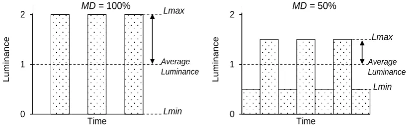
Figure 1.1 Fluctuation of luminance as a function of time for modulation depths of 100 and 50

percent. ... 6

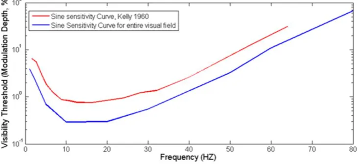
Figure 1.2 Visual Perception Curves (VPC) for the flickering light. ... 7

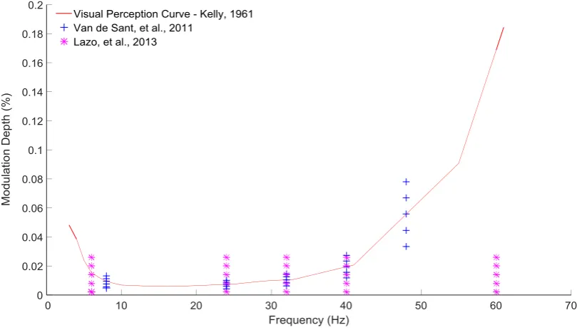
Figure 1.3 The Visual Perception Curve and conditions in two previous related studies ... 8

Figure 3.1 Conditions employed in the current and two related experiments and the Visual Perception Curve ... 13

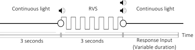
Figure 3.2 Structure of a trial in the flicker perception task. Repetitive Visual Stimulation (RVS) ... 14

Figure 3.3 A participant wearing the EEG cap and the experimental setup. ... 15

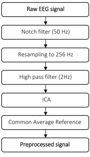
Figure 4.1 Steps in the pre-processing of EEG signal ... 17

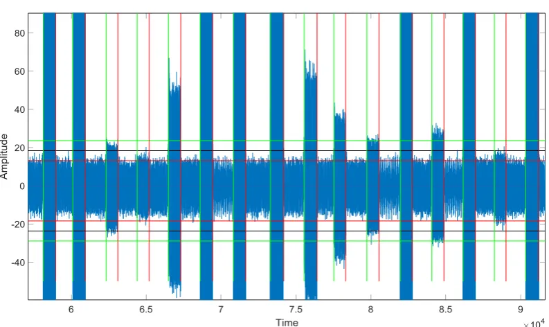
Figure 4.2 Detection of the stimulation events in the photodiode signal. ... 21

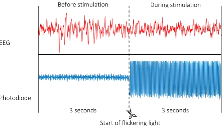
Figure 4.3 Method to segment the epochs. ... 22

Figure 6.1 Power spectrum density average across all participants for each of the conditions at Pz site. ... 28

Figure 6.2 Power Spectrum Density of Pz site averaged for all the participants at the frequency 60 Hz and Modulation Depth 1.4 times the Visual Perception Threshold. ... 30

Figure 6.3 Z-scores score average across subjects at channel Pz channels. Black vertical line represents the frequency of stimulation. ... 28

Figure 6.4 Z-scores topo-plots average for all the participants for the 32 channels. ... 31

Figure 6.5 Distribution of EER values for Pz site for all the participants by frequency. ... 32

Figure 6.6 Distribution of ZEER values for Pz site for all the participants by frequency. ... 33

Figure 6.7 ZEER topo-plots average for all the participants for the 32 channels. ... 34

Figure 6.8 Psychometric function and the underlying binomial distribution for all the frequencies and their corresponding modulation depths (MD). ... 36

Figure 6.9. Visual Perception Curve and the Absolute Modulation and Psychometric Method curves for behavioral responses ... 37

Figure 6.10 ZEER-Psychometric function and the underlying binomial distribution for all the frequencies and their corresponding modulation depths (MD) for the Pz channel. ... 39

Figure 6.11 Visual Perception Curve, Absolute Modulation Depth Curve, Psychometric Curve, and SSVEP Psychometric Curve for Pz. ... 40

Figure 6.12 Visual Perception Curve, and Absolute Modulation Depth Method Curves of Van de Sant, et al., (2011); Lazo, et al., (2013); and Current study. ... 41

(9)

ix Figure 9.1 Power spectrum density average across all the subject for each of the conditions at Oz

site ... 51

Figure 9.2 Z-scores score average across subjects at channel Oz channels ... 52

Figure 9.3 Distribution of EER values for Oz site for all the participants by frequency. Boxplots ... 53

Figure 9.4 Distribution of ZEER values for Oz site for all the participants by frequency ... 54

Figure 9.5 ZEER-Psychometric function and the underlying binomial distribution for all the frequencies and their corresponding modulation depths (MD) for the Oz channel ... 56

Figure 9.6 SSVEP-Psychometric Curve for Oz and the Visual Perception Curve ... 57

List of tables

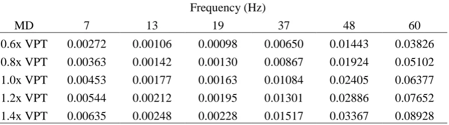
Table 3.1 Absolute values of modulation depth for each frequency in the experimental task ... 13

Table 6.1 Average number of “yes” for all participants per condition ... 35

Table 6.2 Average number of trials with ZEER values greater than 0 for Pz site ... 38

(10)

x

Abbreviations

AMD Absolute Modulation Depth BCI Brain Computer Interfaces CAR Common Average Reference DC Direct Current

EEG Electroencephalography EER Equal Error Rate

FFT Fast Fourier Transforms

ICA Independent Component Analysis MD Modulation Depth

PSD Power spectrum density RVS Repetitive Visual Stimulation

SSVEP Steady State Visual Evoked Potentials VPC Visual Perception Curve

(11)

(12)

1

1 Introduction

The Steady State Visual Evoked Potentials (SSVEP) are electrical responses of the brain to

rapid repetitive stimulation (RVS), also known as flicker. SSVEP are used in research and

practical applications because it is a stable response and reflects characteristics of the

stimulation. The SSVEP is detected at the same frequency, or harmonics, of the driving

stimulation. One way to elicit SSVEP is by flickering light tasks where variations in the

frequency and modulation depth (MD), a measure of light change, of the stimuli are associated

with changes in the SSVEP. However, despite the long history of research on visual perception

and on SSVEP, the effects of frequency and MD on SSVEP are not well addressed and in

particular it still unknown the lowest MD at which SSVEP can be elicited. Such knowledge

will allow to create better tasks to elicit SSVEP and with that potentially increase the accuracy

of SSVEP detection, their use to study the visual system and increase their applications.

This work aimed to find the lowest MD necessary to elicit SSVEP for a variety of

frequencies between 7 and 60 Hz. For this pursue, we used MD proportions (0.6 to 1.4) of the

Visual Perception Thresholds (VPT), the lowest MD at which people can perceive flicker in

the light stimulation. During the task participants had to indicate whether or not they perceived

flicker in light stimulation while simultaneously an electroencephalogram (EEG) was recorded.

We analyzed the EEG data to characterize and measure the strength of the SSVEP. In addition,

we incorporated the results of two earlier related studies in order to increase the number of

frequencies and contribute to create a curve with the lowest MD necessary to elicit SSVEP.

1.1 Steady State Visual Evoked Potentials

Steady State Visual Evoked Potentials (SSVEP) are electrical brain responses associated with

the stimulation of the retina by rapid repetitive visual stimulation (RVS), e.g., flickering light

(Regan, 1977). The main distinctive characteristic of SSVEP is that they contain high power at

the same at the frequency of stimulation and/or harmonics thereof (Regan, 1989). SSVEP have

a very stable amplitude (size) and phase (temporal shift) over time (Regan, 1966) and are most

prominent over occipital cortical areas (Vialatte, Maurice, Dauwels, & Cichocki, 2010).

SSVEP are usually obtained by means of electroencephalographic (EEG) recordings, however

they are also obtained by means of magnetoencephalogram (Thorpe, Nunez, & Srinivasan,

(13)

2 elicited in the absence of a behavioral response and even when participants are not able to

consciously perceive the flicker (Skrandies, & Raile, 1989).

1.2 SSVEP mechanisms

The nature of the mechanisms that generate SSVEP is still unknown. However, there are two

hypothesis that attempt to explain the possible mechanisms underlying SSVEP. These

hypothesis have two different perspectives of SSVEP; they considered SSVEP to be either the

result of spontaneous or evoked oscillations in the brain.

One hypothesis suggests that SSVEP are the result of the enhancement of the

spontaneous oscillations of the brain. This proposes that with RVS stimulation the brain stops

producing its spontaneous neural activity and enters into an entrained state where neurons

synchronize their firing to the stimuli frequency preventing the brain to return to its spontaneous

activity while the stimulation its present (Regan, 1989). This could be explained by the

resonance phenomena, the behavior of neural oscillators of the brain to match stronger some

of their ongoing responses to certain frequencies of period stimulation (Silberstein, 1995, as

cited in Bayram, et al., 2011).In one study, dedicated to evaluate this hypothesis, frequencies

from 1 to 100 Hz with an increase of 1 Hz were tested in a flicker perception task (Herrmann,

2001). It was found that participants present stronger responses to 10, 20, 40 and 80 Hz

compared to the other frequencies, even when the stimuli at these frequencies were not different

to the rest of the stimuli. This results suggest that SSVEP could be the result of tuning of

ongoing oscillations of the brain to certain frequencies.

The second hypothesis suggests that SSVEP are the result of induced responses

provoked by stimulation. According to this this hypothesis SSVEP might be the result of the

addition of individual and small transient responses, such as Event-Related Potentials (ERPs),

generated by each stimulus (Capilla, Pazo-Alvarez, Darrriba, Campo & Grosss, 2011). This is

similar to explanation of the generation of early ERPs by phase resetting behavior of neurons

(shifts in their dynamic oscillations) instead of additive amplitude changes (Makeig et al.,

2002). A recent study found that SSVEP could be explained by phase resetting (Moratti,

Clementz, Gao, Ortiz, & Keil, 2007). In that study the changes on amplitude and phase,

associated with SSVEP, before and after the start of stimulation were tracked. They found few

changes in amplitude but a strong phase alignment, which suggest that phase alignment could

(14)

3

1.3 SSVEP neurophysiology

The three components of the visual system - the retina, the visual path and the visual cortex-

are expected to be involved in the generation of the SSVEP. However, due to the low spatial

resolution of the EEG, which is the main technique for obtaining SSVEP, the mechanisms in

the visual cortex and in the rest of the visual system are vastly unknown. According to Vialatte

and colleagues (2010) the three main visual pathways - the magnocellular, the parvocellular

and the koniocellular – take part in the generation of the SSVEP. The three pathways start in

the retina continue to the lateral geniculate nuclei and project to the visual areas, an in particular

the striate cortex (V1), which is considered to be the strongest local source for SSVEP (Vialatte,

et al, 2010). LGN activation has been found to be associated with the generation of SSVEP

(Krolak-Salmon et al., 2003).

SSVEP could also have contribution from other cortical and subcortical regions, from

the primary visual cortex the SSVEP could propagate to other brain areas. This idea is

supported by the findings that regions beyond the visual system are activated during SSVEP,

these areas include parietal and frontal brain areas (Srinivasan, Bibi, & Nunez, 2006; Pastor,

Valencia, Artieda, Alegre, & Masdeu, 2007) and the cerebellum (Pastor, Artieda, Arbizu,

Valencia, & Masdeu, 2003). It appears that SSVEP manifest in an occipito-frontal network

that is connected to certain extra-cortical structures (Srinivasan, Fornari, Knyazeva, Meuli, &

Maeder, 2007).

1.4 SSVEP characteristics

SSVEP have several distinctive properties that make them a strong and objective measure of

brain response: a) the experimenter has control over the SSVEP as one can manipulate variables

that affect the SSVEP such as spatial frequency, luminance, and hue (Di Russo, Spinelli, &

Morrone, 2001), b) SSVEP are less susceptible than ERPs to artifacts produced by eye

movements (Perlstein, et al., 2003) and to electromyographic noise contamination (Gray,

Kemp, Silberstein, & Nathan, 2003) c) SSVEP are an implicit response as they do not require

a motor response to be elicited and as a result are not highly influenced by effects after sensory

or perceptual encoding stages (Skrandies, & Raile, 1989), d) they have a high signal to noise

ratio (SNR) particularly in occipital sites as only a fraction of the noise contained in the EEG

affects the SSVEP frequency related to the stimulus and at high frequencies the noise is lower

(15)

4 valid measure of brain activity as they are elicited by a continuous sustained visual experience

rather than by an isolated stimulus (Di Russo, et al., 2007).

1.5 SSVEP applications

The above distinctive characteristics make SSVEP very useful for research and also practical

purposes. In cognitive neuroscience, SSVEP are often used to indirectly estimate the

propagation of brain activity on a cognitive task (Vialatte, et al., 2010). Some cognitive

processes that have been studied through the use of SSVEP include visual attention (Morgan,

Hansen, & Hillyard, 1996), binocular rivalry (Müller, et al., 1998) and working memory

(Perlstein et al., 2003). In clinical neuroscience SSVEP are used as a diagnostic tool to study

pathological brain dynamics. For instance, it was found that the magnocellular pathway is

affected in patients with Alzheimer. This was found by evaluating the visual system with the

use of SSVEP elicited by stimulation at high frequencies (Sartucci, et al., 2010).

However, by far the main practical application of SSVEP is in the field of Brain

Computer Interfaces (BCI). The objective of BCI is to establish a direct communication

between a brain and a computer that allows a person to control or communicate with a device

without muscular intervention (Van Erp, Lotte, Tangermann, 2012). The main reason SSVEP

are used in BCI is because the frequency of the stimulation can be reliably and quickly

recognized in the SSVEP frequency domain. Other characteristics that make SSVEP very

suitable for BCI are that they have a very high temporal resolution for data acquisition (~0.05

seconds; Nicolas-Alonso, & Gomez-Gil, 2012), people require minimal training to perform a

SSVEP task (Vialete, et al., 2010), the cost of the SSVEP necessary equipment is low compared

with other neuroscience techniques (Luck, 2014), there are years of research on SSVEP and

BCI (Norcia, et al., 2015), and SSVEP allow people a relatively free movement of their head

and eyes compared with other neuroscience methods such as eye tracking.

A common example of a SSVEP-based BCI application is the control of a wheelchair.

In a BCI-controlled wheelchair system, four sources of light can be associated with four

directions: up, down, right and left. When a person wants to move the chair in a certain direction

they need to attend the light stimulus associated with that command. The computer program

would analyze the brain activity, identify the frequency of the SSVEP and send the command

(16)

5

1.6 SSVEP limitations

Despite the strengths of the SSVEP, they also have some side effects and disadvantages. One

disadvantage of SSVEP is the possibly harmful side effects of the exposure to fluctuating light.

It has been documented that a few seconds of exposure to flickering light with bright colors at

low to medium frequencies can trigger epileptic seizures (Fisher, Harding, Erba, Barkley, &

Wilkins, 2005). One of the most infamous cases is the one of the Japanese cartoon "Pokémon”.

In an episode repetitive visual stimuli induced photosensitive epileptic seizures in hundreds of

viewers (Ishiguro, et al., 2004). Furthermore, high frequencies may also have other undesirable

effects. It has been reported that long (5 minutes or more) and continuous exposure to flickering

light at unperceivable high frequencies can induce migraines (Vanagaite, et al., 1997) or

impaired visual performance in an office environment (Kuller, & Laike, 1998).

The influence of sensorial and cognitive processing on the perception of RVS and

subsequently on SSVEP are also not very well addressed. Habituation and attention are only

two examples of processes that can influence SSVEP. Prolonged view of flickering stimulation

at a particular frequency causes adaptation (Pantle, 1971), which can already reduce the EEG

amplitude (Bergholz, Lehmann, Fritz & Rüther, 2008). The perception sensitivity to RVS at

low or medium frequency (e.g., 30 Hz) can be reduced to by adaptation to a higher

unperceivable flickering stimulation (e.g., 60 Hz) (Shady, MacLeod, & Fisher, 2004). Visual

attention is also associated with pupil dilation which could increase retinal luminance and affect

the effectiveness of an SSVEP stimulus (Janisse 1997 in Silberstein, et al., 1990). SSVEP are

also enhanced by selective attention to an attended versus and unattended stimulus (Morgan,

Hansen, & Hillyard, 1996).

1.7 SSVEP tradeoff strength and discomfort

For SSVEP based BCI applications and to reduce the possible side effects of flickering light,

the RVS is preferred to elicit strong SSVEP responses, while not causing visual discomfort to

people. It should be pointed out that this is not always the case, for instance in for clinical

applications where the goal is to test integrity of the visual pathway like in patients who suffered

epileptic seizures, RVS may be preferred to cause discomfort to people (Trenité, Binnie, &

Meinardi, 1987). The case of RVS for SSVEP-based BCI is a difficult endeavor, due to the fact

that both stimulation at low and high frequencies have their advantages and disadvantages.

(17)

6 discomfort as people can perceive the flicker, however the SSVEP amplitude is greater for low

frequencies stimulation, particularly around the EEG alpha range (8–13 Hz), where the SSVEP

signal has the highest amplitude (Regan, 1989). On the other hand stimulation at high

frequencies and at medium to low MD (smaller than the MD at the VPT) are less uncomfortable

to people as the stimulation is perceived as continuous, but this frequency range and MD

induces weaker or no SSVEP responses (Van de Sant, et al., 2011).

1.8 Visual perception and SSVEP

SSVEP are very sensitive to characteristics of the stimulus such as spatial frequency,

luminance, and color (Di Russo, Spinelli, & Morrone. 2001). Among those characteristics, the

frequency and MD are particularly relevant as they modulate the amplitude of SSVEP (Regan,

1989). The frequency measured in (Hz) is the number of repetitions of the stimulus per unit of

time (seconds). MD is a measure of light variation that quantifies the relation between the

spread and sum of two luminances during period oscillations (Perz, et al., 2011). For a

time-varying luminance, such as flickering light, MD is an indication of the ratio between the

average light level and the amount of change in the light and can be calculated according to the

equation 1.1. In addition, the concept can be visualized in Figure 1.1.

MD = * 100 Lmax - Lmin

Lmax + Lmin

where:

MD = Modulation Depth

Lmax = maximum luminance

Lmin = minimum luminance

Eq. 1.1 0 1 2 Lu m ina nce Time Lmax

MD = 100%

Lmin Average Luminance 0 1 2 Lu m ina nce Time Average Luminance Lmax

MD = 50%

[image:17.595.84.502.570.697.2]

Lmin

(18)

7 In addition, frequency and MD determine the human perception of RVS and such

relationship is described by the temporal contrast sensitivity function (Kelly, 1961). The curve

is known as Visual Perception Curve (VPC) and it defines the Visual Perception Threshold

(VPT)in terms of frequency and MD. A VPT is the lowest MD for a particular frequency at

which people can perceive RVS as discontinuous. Usually people perceive as discontinuous

stimulation RVS with MD on and above the VPT and as continuous stimulation RVS with MD

below the VPT. From frequencies above 10 Hz the VPC has an increase in MD with an increase

in frequency. For instance, at low frequencies (e.g., 10 Hz) only small changes in MD are

necessary for people to detect the RVS as discontinuous. While at high frequencies (e.g., above

40 Hz), higher MD are required for people to detect the RVS as discontinuous (Figure 1.2).

A more recent version of the VPC, using the entire visual field and controlling for

adaptation was created recently at Philips Research (Perz, Sekulovski, & Vogels, 2011). The

recent VPC has a similar shape to the Kelly’s curve (1961), but it has lower VPTs. The two

curves can be seen in Figure 1.2.

We consider the VPC by Perz and colleagues (2011) to be more appropriate than the

VPC by Kelly (1961) for our study because of the following reasons: Perz and colleagues

evaluated the a visual field of 137° in a binocular experiment instead of the only 65 ° in Kelly’s

monocular experiment, they controlled for adaptation in the experimental task as they used a

staircase detection task, instead of the tuning methodology of Kelly. In the Perz and colleagues Figure 1.2. Visual Perception Curves (VPC) for the perception of

[image:18.595.118.484.392.560.2]

(19)

8 detection task MD increased or decreased until the participant response change from “yes” to

“no” or vice-versa which prevent for adaptation. In both studies stimuli were presented centrally on the retina. Moreover, the Perz’s study has an additional advantage for our study,

we can use the same setup they used because their equipment is at our disposal at Philips

Research, and that set up has been used in related relevant studies.

1.9 The Visual Perception Curve and SSVEP

To our knowledge there are few studies that investigated how the frequency and MD of the

RVS affect the SSVEP (Van de Sant, et al., 2011; Lazo, et al., 2013). Van de Sant et al. (2011)

exposed participants to RVS light at frequencies of 8, 24, 32, 40 and 48 Hz and MD of 0.6, 0.8,

1.0, 1.2, 1.4 times the VPT in Kelly’s VPC (1961). They found SSVEP for all the frequencies,

except 8 Hz, at MD starting below the VPT. In the second study, Lazo et al. (2013) investigated

five frequencies 6, 24, 32, 40, 60 Hz at five absolute MDs 0.002, 0.008, 0.014, 0.020, and 0.026.

They found SSVEP only for the frequencies 24 and 32 Hz at MD starting at 0.008 and for 40

Hz at MD starting at 0.002. SSVEP were not found for the lowest frequency 7 Hz, nor for the

highest frequency 60Hz. A visual representation of the conditions in these two studies can be

seen in Figure 1.3.

[image:19.595.82.487.465.696.2]

(20)

9

2 Purpose of the study

Since the first time SSVEP were characterized (Adrian & Matthews, 1934), they have been a

useful tool to study the brain activity associated to visual perception (Reagan, 1989) and in the

last decade their use have increased to more practical applications (see a review Norcia, et al,

2015). However, one issue concerning SSVEP that has not been addressed is regarding the

neural model describing the human sensitivity to the perception of RVS. The effect of

frequency and MDs and in particular the value of the lowest MD necessary to elicit SSVEP are

unknown. That knowledge could help increasing the accuracy of SSVEP detection and help to

develop better models to evaluate the visual system and also increase their applications.

However, besides the two studies conducted at Philips Research we have no knowledge of

research addressing this issue.

We considered that investigating the effect of the driving frequency on SSVEP and in

particular finding the lowest MD necessary to elicit SSVEP are particularly relevant for the

research and the practical application of SSVEP. That can help to develop better task

minimizing any adverse effect from RVS.

2.1 Objectives of the study

We aimed to study the effect of frequency and MD on SSVEP and to find the lowest MDs

necessary to elicit SSVEP for frequencies in the range of the VPC (1 to ~70 Hz) and with that

help to create a SSVEP contrast sensitivity curve, a curve with the values of the lowest MD

necessary to elicit SSVEP for a wide range of frequencies. We also aim at examining the

interaction between different range of frequencies (low, medium and high) and MD (below, at

and above the VPT) and find if they affect SSVEP in a similar manner as in the visual

perception research: an increase in frequency requires an increase in MD.

Thus, we have three goals in this study. The first goal is to investigate it is possible to

elicit SSVEP around the VPC, and if so for what frequencies and MDs. In particular we are

interested to find the lowest MD necessary to elicit SSVEP. The second goal is to examine how

the interaction between frequency and MD affect SSVEP. The third goal is to create a SSVEP

contrast sensitivity curve by combining our results with the two previous related studies.

We intend to use the Perz’s VPC (Perz, et al, 2011) as we mentioned in the introduction

section is better suited for our study than the Kelly’s VPC (Kelly, 1961). From here on, we will

(21)

10

2.2 Research questions

1. Is it possible to elicit SSVEP with MDs proportions (0.6 to 1.4) of the VPT for

frequencies in the range of 7 to 60 Hz by RVS light? If yes, for what frequencies and

MDs and what are the lowest MDs necessary to elicit SSVEP?

2. How do the frequency and MD of the RVS affect SSVEP?

3. Is the SSVEP contrast sensitivity curve similar to the VPC?

2.3 Hypothesis

1. SSVEP are elicited by RVS with MDs around the VPT. However this occur only for

MDs that are equal of higher than the VPT for SSVEP. The lowest MDs necessary to

elicit SSVEP are above the VPT of the VPC.

2. There is an interaction between frequency of stimulation and MD: an increase in

frequency requires an increase in MD to elicit SSVEP. We expected the SSVEP-VPC

follows a similar pattern to the VPC.

1. The MD necessary to elicit SSVEP at high frequencies is higher than the VPT

at low frequencies.

2. There is a high increase in MD necessary to elicit SSVEP for frequencies higher

than 30 Hz as in the VPC.

3. The SSVEP contrast sensitivity curve has a similar shape to the VPC. However, the

(22)

11

3 Methods

We created RVS light perception task with 6 different frequencies in three frequency ranges

low, medium and high (7, 13, 19, 37, 48 and 60 Hz ) combined with 5 MD proportions of the

VPT (0.6, 0.8, 1.0, 1.2, and 1.4).

3.1 Participants

The group of participants consisted of 24 healthy volunteers (17 males and 7 females, Mean

age = 26.4; SD = 6.0). The participants were recruited among the Philips Research employee

population at High Tech Campus, Eindhoven. All participants had normal or corrected to

normal vision. At the end of the experiment participants were rewarded with chocolate and a

hair wash coupon to remove the gel used during EEG recording. Three additional participants

were excluded from the final group due to problems with the EEG recording (n =2) or recording

the RVS events (n = 1).

3.2 Inclusion and exclusion criteria

In order to be included in the study, participants had to be between 20 to 50 years old. They

also had to be healthy: no vision related problem, no history of epilepsy, neurophysiological

disorder, migraine, or sleep problems. Participants were excluded in case of: colorblindness,

suspicion or report of an aberrant light sensitivity, photosensitizing medication, sleep disorders

or visual impairments.

3.3 Ethical considerations

The research protocol was approved by the Philips Research Ethics committee board (Internal

Committee Biomedical Experiments). Prior to the study, participants received a consent letter

with all details related to their involvement in the study. At the start of the study the participants

signed the letter.

3.4 Materials

The experimental setup consisted of the following hardware: a) 2 LED panels 57.5 cm x 57.5

cm equipped strips of white lamps, b) Agilent N3300A System DC Electronic Load, c) Agilent

(23)

12 electrode setup placed on a textile cap according to the international 10-20 system, f)

Photodiode, g) Laptop with Windows 7 operating system, h) 18-Key USB Numeric Keypad.

The RVS light was presented via a custom made program in JAVA. The waveform

specifications were sent to the Agilent 33522A function generator and then to the LED panels

using the TCP/IP interface. Once the waveforms were created, they passed through the Agilent

N3300A System DC Electronic Load in order to regulate the current load before they reached

the lamps. The light stimulation was reflected on a white wall with a fixation cross in the

middle. The participants were instructed to look at the fixation cross during the experiment.

The USB numeric Keypad was connected to the Laptop to receive the input from the

participants. The BioSemi ActiveTwo EEG Acquisition System recorded the EEG and the light

stimulation signals via the use of an EEG cap and a photodiode respectively. All data were

saved on the laptop.

3.5 Stimuli

The light stimulation was delivered via two LEDs panels with a size of 57.5 cm x 57.5 cm and

equipped with four rows of cold warm white LEDs. For this experiment only the cold LEDs

were used. The LEDs panels were suspended on a stand at a height of 2.5 and illuminated a

white wall in front of the participant. The LEDs panels were controlled via an Agilent function

generator. The system was calibrated to ensure that the correct output was delivered. The light

stimulation covered a total area of approximately 210 cm x 360 cm (vertically x horizontally).

Participants were at a distance of 70 cm and have a visual angle of 137°. These devices for light

stimulation resemble the conditions of a typical office and have worked properly in previous

experiments at Philips Research.

3.6 Stimulus selection and design

The 30 conditions were created from the combination of 6 frequencies (7, 13, 19, 37, 48 and

60 Hz) and 5 MD (0.6, 0.8, 1.0, 1.2, and 1.4) times the corresponding VPT of each frequency

at the VPC. The absolute values of the MD are listed in Table 3.1.

The selection of these frequencies and MDs was motivated by our aim to combine our

results with the two previous related studies (Van de Sant, et al., 2011; Lazo, et al., 2013), which

allowed us to have more conditions around the VPC. The conditions of the previous and our

(24)

13 medium (12-30 Hz) and high frequencies (>30 Hz), and to cover areas that were not covered

in the previous studies.

We chose in this study square waves, instead of sine waves, because square waves were

[image:24.595.78.526.180.305.2]

used in the two previous related studies we intended to combine our results and because square Table 3.1

Absolute values of modulation depth for each frequency in the experimental task

Frequency (Hz)

MD 7 13 19 37 48 60

0.6x VPT 0.00272 0.00106 0.00098 0.00650 0.01443 0.03826

0.8x VPT 0.00363 0.00142 0.00130 0.00867 0.01924 0.05102

1.0x VPT 0.00453 0.00177 0.00163 0.01084 0.02405 0.06377

1.2x VPT 0.00544 0.00212 0.00195 0.01301 0.02886 0.07652

1.4x VPT 0.00635 0.00248 0.00228 0.01517 0.03367 0.08928

Note. MD = Modulation Depth; VPT = lowest MD at which participants perceive RVS as discontinuous, the values were obtained from the Visual Perception Curve (Perz, et al., 2011); x = times, for instance 0.6x VPT is equal to 0.6 times the VPT

[image:24.595.111.505.386.614.2]

(25)

14 waves have a higher accuracy than sine waves for eliciting SSVEP at the frequency of

stimulation (Teng, et al., 2011). The waves had a duration of 3 seconds (6248 samples at a

sample rate of 2048Hz). The average light luminance level was 1000 Lux and the color

temperature was 4000 K. The waveforms were created using the following equation:

3.7 Experimental Task

The experimental task consisted of 300 trials that were the result of 30 RVS waveforms that

were repeated 10 times each. A trial consisted of 3 seconds of continuous light, followed by a

beep and 3 seconds of RVS which were followed by 2 beeps and a period of continuous light

that continued until the participant gave a response. See Figure 3.2 for a visual representation

of one trial.

The trials were randomly organized for each participant in three blocks of 100 stimuli.

Each block lasted approximately 14 minutes and was followed by a break of a variable duration

(3-10 minutes). Participants respond whether or not they perceived flicker by pressing “yes” or

“no” stickers over the buttons on a number pad (6 for “yes” and 4 for “no”).

Waveform = AvLL + square (T* F) * MD * AvLL

where:

AvLL = Average Light Level

square () = square waves T = Time (seconds) F = Frequency (Hz)

MD = Modulation Depth (%)

Eq. 3.1

3 seconds 3 seconds Response Input

(Variable duration)

[image:25.595.97.503.473.578.2]

Continuous light RVS Continuous light

Figure 3.2. Structure of a trial in the flicker perception task. Repetitive Visual Stimulation (RVS).

(26)

15

3.8 Experimental session

The study consisted of one experimental session of approximately one hour and fifteen minutes.

At the beginning of the session the experimental leader explained the goal of the study and

answered any questions that participants had regarding the procedures to be conducted during

the session. After that participants were seated comfortably on a chair in front of the white wall

where the light was reflected. Then, we proceeded with placing an EEG cap on the head of the

participant, and added conductive gel to the electrodes. Next, we measured the impedances of

the EEG signal, and made sure the impedances of all the channels were below 20 µV.

Once the EEG cap was set, participants were again explained the task they needed to

perform and were allowed to do a short practice run. During the experiment participants were

instructed to look with their two eyes open at a fixation cross on the middle of the wall. Between

blocks participants had a break where they had the opportunity to relax and drink some water.

At the end of the session the experimental leader answered any questions that the participants

had regarding the experiment. Also, the experimental leader gave the participants a chocolate

[image:26.595.171.432.419.606.2]

and a hair wash coupon to remove the gel left in their hair.

(27)

16

4 Data collection

Electrical brain activity was recorded from 32 scalp sites (Fp1, AF3, F7, F3, FC1, FC5, T7,

C3, CP1, CP5, P7, P3, Pz, PO3, O1, Oz, O2, PO4, P4, P8, CP6, CP2, C4, T8, FC6, FC2, F4,

F8, AF4, Fp2, Fz, and Cz) positioned according to the international 10-20 system using an

elastic cap. The signals were recorded at a sampling rate of 2048 Hz using the BioSemiTM

ActiveTwo signal acquisition system (BioSemi products, 2016, July 16). Two additional

electrodes, a Common Mode Sense active electrode and Driven Right Leg passive electrode

were used to replace the ground and references electrodes respectively.

The flickering light was recorded using a photodiode that recorded the variations of the

light reflected in the wall. Large variations in the average light were used to identify the start

and the end of the trials. After the experiment, the events were detected in the photodiode.

Then, the time of the start and the end of the events were marked in the EEG signal. This

process is explained later in the preprocessing section. The photodiode was placed in a small

table at the left side of the participants at a distance of approximately 70 cm to the wall. In

addition, the behavioral responses of the participants were logged in a text file together with

the frequency and MD of the corresponding trial.

4.1 Data pre-processing

EEG and light signals were preprocessed using EEGLAB (Delorme & Makeig, 2004) and

custom-made MATLAB scripts. We followed the procedures employed in the two previous

related studies (Van de Sant, et al., 2011; Lazo, et al., 2013). Signals were notch filtered at

power-line frequency (50Hz) and then re-sampled at 256 Hz. Then, signals were high pass

filtered at 2Hz and blinks components were removed by Independent Component Analysis

(ICA). After that signals were referenced to common average reference (CAR) excluding T7

and T8 channels. Finally, the data was separated into non overlapping epochs. The

(28)

17

4.1.1 Notch filter (50 Hz)

The preprocessing started by removing the external noise that comes from the AC power line.

For this purpose we applied a notch filter at 50 Hz to remove the external noise coming from

the AC power line.

4.1.2 Resampling

The original rate of the recording of each measurement point, called sample, was at 2048 Hz.

This implies that for each second we had 2048 points of information, which requires a long

time for processing. So as to reduce the time necessary to process the signal, we resample from

the original 2048 Hz to 256 Hz.

4.1.3 High pass filter (2 Hz)

The EEG signal below 2 Hz is often affected by drifts in the impedance of electrodes and

sweating. In order to reduce those effects a high pass filter with a cutoff at 2 Hz was applied by

a linear-phase finite impulse response (FIR) filter to eliminate DC shifts (Widmann, Schröger,

& Maess, 2015).

Raw EEG signal

Notch filter (50 Hz)

Resampling to 256 Hz

High pass filter (2Hz)

Common Average Reference ICA

[image:28.595.217.373.67.339.2]

(29)

18

4.1.4 Independent Component Analysis (ICA)

The EEG signal is susceptible to eye blinks and other artifacts, which represents an issue to its

adequate interpretation and analysis. The ICA technique separates the different sources of the

EEG signal and with that helps to remove the contribution of these artifacts. For ICA we

followed the procedure employed by Lazo, et al., (2013), the equations presented below were

taken and adapted from their study. The artifact correction extracts from the recorded signal

the information that corresponds exclusively to cerebral sources. The signal can be represented

as the following equation:

ICA is a blind source separation method that enables representing the data as a linear

combination of statistically independent signals (sources). The artifact components of an EEG

signal can be estimated by ICA, if we assume that the potentials of artifacts in EEG are

independent from cerebral EEG potentials, the artifacts and signals. ICA can be explained with

the cocktail-party problem (Hyvärinen, Karhunen, & Oja, 2001) and the signal can be modeled

according to the following equation:

The goal is to estimate the mixing components and coefficient from the recorded signal. The model can be written as follows:

𝐸𝐸𝐺_𝑟𝑒𝑐 𝑡 = 𝐸𝐸𝐺𝑐 𝑡 + 𝐸𝐸𝐺𝑛 𝑡 𝑁

𝑛=1

where:

𝐸𝐸𝐺_𝑟𝑒𝑐 𝑡 = recorded EEG signal 𝐸𝐸𝐺_𝑐 𝑡 = signal from cerebral sources 𝐸𝐸𝐺_𝑛 𝑡 = signal from artifactual sources

Eq. 4.1

𝑥_𝑖 𝑡 = 𝑎𝑖1𝑠1 𝑡 + 𝑎𝑖2𝑠2 𝑡 + ⋯ + 𝑎𝑖𝑛𝑠𝑛 𝑡 for all 𝑖 = 1, … , 𝑛,

where:

n: number of people speaking simultaneously in a room and number of microphones

𝑥𝑖 𝑡 : microphone measure

𝑠_𝑛 𝑡 : speech signal emitted by the speaker

𝑎_𝑖𝑗: distance (parameter) between the microphones and speakers

Eq. 4.2

Eq. 4.3

(30)

19 The components 𝑠_𝑖 𝑡 are inversely given by:

Then, by assuming certain restrictions on s and M it is possible to estimate them. The assumptions of ICA on the sources sn are:

1. All the sources are mutually independent to estimate W

2. All but one component must have non-Gaussian distributions

3. The number of independent components is equal to the number of observed mixtures

4.1.5 Common Average Reference (CAR)

CAR is a spatial filter that creates a common average with the values of all the electrodes and

subtract that value from each channel. CAR works as a filter that reduces the activity that is

present in large sections of the electrodes. The CAR method has proved to be comparable with

the ear-reference method for referencing (McFarland, McCane, David, & Wolpaw, 1997). The

CAR was computed with the following equation:

After these steps the pre-processed signal was saved in separated files for each participant.

V_iCAR _{= V} iER−

V_jER n j=1

n

where:

𝑉_𝑖𝐸𝑅_{= to the potential between the}_i_{th channel and the reference}

n = to the number of channels in the montage.

Eq. 4.6 Eq. 4.5

s=Wx,

where:

W = to the M (unmixing matrix) where:

x = is a vector with 𝑥1 𝑡 , … 𝑥𝑛 𝑡 as elements

M = is an n x n Matrix with 𝑎1 𝑡 , … 𝑎𝑛 𝑡 as elements

s = is a vector with 𝑠1 𝑡 , … 𝑠𝑛 𝑡 as elements

𝑥 = 𝑎_𝑖𝑠_𝑖

𝑛

𝑖=1

(31)

20

4.1.6 Data segmentation and averaging

Once the signal was preprocessed, first we identify the start and the end of the 3 seconds of

RVS stimulation in the photodiode signal. Then we saved the information regarding the start

and the end of the events detected in the light signal and added that info to the EEG signal.

Then, these epochs on the EEG signal were segmented.

4.1.7 Identify events in photodiode signal

With the use of a photodiode we recorded the light stimulation during the entire session

simultaneously and at the same sampling rate as the EEG signal. In the light signal we identify

the stimuli by finding large changes in the average signal that correspond to the presentation of

the stimuli.

With a custom made script we set a threshold, line red in Figure 4.2, and searched for

peaks that crossed that threshold. Once we found a peak that crossed the threshold we evaluated

if the 767 following consecutive points also crossed the threshold (768 in total which

correspond to the length of the 3 seconds of stimulation). If any of the 767 following points did

not cross the threshold we searched for the next point that crossed it and repeated the procedure.

If 768 consecutive points crossed the threshold, we consider them to be an event, and we

marked the first (green vertical line) and the last (red vertical line) point, that match to the start

and the end of the stimuli. We saved that data to later overlap with the EEG signal and use it

as a reference for EEG processing.

Most of the 300 trials during the experiment were detected automatically with the above

mentioned script that searched for differences in the average light. However, some events were

not detected because the change in the signal was small compared with the average light

(continuous light). These events were usually events in the low frequencies and low MD

conditions of the experiment. This happened in around 10 percent of the total events per

participant. For those not detected events, we proceeded to manual detection that consisted on

visual inspection for variation in the signal and manual noting the start and the end of each

event and then merging those with the automatically detected events. This manual correction

was very time consuming and required a considerable amount effort, but we were able to detect

(32)

21

4.1.8 Epochs segmentation

The events detected in the previous step were used to extract epochs from the EEG signal

corresponding to the RVS. The EEG signal was separated into non-overlapping epochs of 6

seconds. This period correspond to 3 seconds after the start of stimulation and 3 seconds before

the start of stimulation (see Figure 4.3).

4.1.9 Reject epochs

The artifacts were rejected after analyzing the energy of the signal. EEG signal with peaks

higher than the sum of the mean of the signal and four times the standard deviation of the signal

were rejected in order to exclude trials contaminated with motor or other artifacts. This criteria

is represented in the equation 4.7.

[image:32.595.99.496.81.317.2]

(33)

22 EEG

Photodiode

Start of flickering light

Figure 4.3. Method to segments the epochs. The method consists of detecting the start of the flickering light (stimulation) in the photodiode signal and using it as a reference. Two sets of epochs are created with the reference of 3 seconds, before and after the stimulation.

Before stimulation During stimulation

3 seconds 3 seconds

Eq. 4.7

EpochVar < {meanVar(channel) + 4*stdVar(channel)} where:

channel = channel number

EpochVar = variance of the current epoch

meanVar(channel) = variance of the mean of the current channel across all conditions

[image:33.595.99.459.75.279.2]

(34)

23

5 Data Analysis

In the data analysis we followed the procedures employed in the two previous related studies

(Van de Sant, et al., 2011; Lazo, et al., 2013) that has been developed in Philips Research

because they proved to be effective to detect SSVEP and because this facilitates the

combination of their results with ours. The data analysis consisted of the following steps: 1)

Power spectral density, 2) Z-score, 3) Equal Error Rates, and 4) Z-score at the Equal Error Rate.

This analysis allowed us to estimate the strength of the SSVEP and investigate their relationship

with visual perception. This section gives a brief explanation of each method.

5.1 Power Spectral Density (PSD)

PSD is a measure of the power of a signal in the frequency domain. PSD is calculated from the

Fast Fourier Transform (FFT) of a signal and it provides a way to characterize the amplitude

versus frequency content of the EEG signal.

We applied the FFT into segmented successive time block windows instead of the full

epochs. Our epochs had a duration of 3 seconds (768 samples at a sampling rate of 256 Hz): 3

seconds before the start stimulation onset (baseline) and 3 seconds after the start of stimulation

(RVS). We used a window of length of 256 samples and an overlap of 128 samples (0.5

seconds). This procedure resulted in 5 half overlapping windows with a length of 256 samples

for each 3-second long interval (before and during stimulation).

To plot the data, we selected a channel of interest and take the PSD MATLAB structure,

where the values are stored in a 129 length vector. Each data point correspond to one frequency

from 1 to 1-128 Hz. Next, we took the mean of the all the PSD epochs that correspond to a

condition and we plotted the conditions in the frequency domain. The same procedure was

applied for the segments before and after the start of the stimulation. The power of PSD in the

plots is represented in microVolt^2/Hz. The Hz unit depends on the frequency resolution, and

in our case it was 0.333 Hz the resolution, so our unit for PSD is uV^2/0.33 Hz.

5.2 Z-scores

Z-scores (standardized scores) were used to estimate the intensity of the SSVEP response. An

individual Z-score was calculated for each trial during stimulation by comparing the PSD log

(35)

24 of their trials was subtracted by the mean of all baseline trials and then divided by the standard

deviation of all the baseline trials (see equation below):

5.3 Equal Error Rate (EER)

To determine whether or not SSVEP were elicited due to the RVS, we found the point at which

the probability of type I error is equal to the probability of type II error. This point is the one at

which the False Positive (FP) and False Negative (FN) rates are the same. We call this point

the Equal Error Rate (EER) and it is calculated according to the equation 5.2 shown below.

EER are very useful for biometric systems, like the EEG, to have an optimal identification of

the information collected by the device. The lower the equal error rate value, the higher the

accuracy of the measurement.

5.4 Z-score at the Equal Error Rate (ZEER)

The Z-scores allow to determine the existence of statistically significant difference between

two samples that are normally distributed (in our case the log PSD). The multiplication of the

standard score and EER gives us a balanced combination of both extracted features to define

the measure of the SSVEP intensity.

Zscore = x - 



where:

x= log PSD’s epochs of one trial during stimulation

 = mean of log PSD’s epochs of all trials before stimulation

 = standard deviations of log PSD’s epochs of all trials

before stimulation

Eq. 5.1

Eq. 5.2

where:

1= mean of log PSD’s epochs of all trial during stimulation

2 = mean of log PSD’s epochs of all trials before stimulation

 = standard deviations of log PSD’s epochs of all trials

); * 2 ( 1 2

 

 

 p

(36)

25 The measure of the intensity of SSVEP, based on a low standard score can be boosted

by the EER in case that the distribution of the samples during and before stimulus has a small

overlap. On the contrary, a high SSVEP intensity measure based on a high standard score can

be reduced if there is a big overlap in the distributions. The ZEER unit (z-scores at the EER)

was computed as follows:

5.5 Estimation methods for sensitivity curves

We created sensitivity curves with the use of the behavioral data and the SSVEP signal. The

sensitivity curves we created are our approximations to the VPC (Perz, et al., 2011). The

sensitivity curves contains the lowest MD necessary for people to perceive the flicker for the

behavioral data and to elicit SSVEP for the SSVEP signal. To create these curves we made use

of the absolute modulation depth and the psychometric method. We provide a description of

these methods in the following paragraphs.

5.5.1 Absolute Modulation Depth (AMD) method

The AMD method finds the lowest MD for a certain frequency that passes a predefined

threshold. We set this threshold at 50% of the total responses for a condition (a frequency and

a MD) for both behavioral responses and SSVEP. This 50% detection rate in “yes/no” task is

often called detection threshold and it is considered not to be reached by guessing (Rose, Teller,

& Rendleman, 1970). Moreover, this threshold has used in previous related studies (Lazo, et

al., 2013; Perz, et al., 2011; Van de Sant, et al., 2011).

In the case of behavioral responses, for a condition, the threshold was reached when in

at least half of the trials participants indicated that they perceived flicker (i.e. 5 out of 10 trials).

In the case of the SSVEP the threshold was reached when in half of the trials the ZEER values

where higher than 0. A ZEER values higher than 0 is an indication than the SSVEP was detected

by our method.

if EER ≥ 0.5 or Z-score ≤ 0 then ZEER = 0

if EER ≤ 0.5 or Z-score ≥ 0 then ZEER = Z-score * (1 – EER)

(37)

26

5.5.2 Psychometric method (PM)

The Psychometric method makes use of the non-linear square regression model. With the use

of regression analysis the observed data is modeled by a parametric function in order to estimate

the coefficients of the nonlinear regression function. As in the case of the AMD we set the

selection threshold at 50 % of the trials for a condition “yes” responses for behavioral data and

50 % of ZEER values greater than 0 for SSVEP data. The equation for the Psychometric

function is shown below:

Eq. 5.4

L(x; α, β) = 1 1 + _𝑒𝑎−𝑥𝛽 where:

definition range: x ϵ (-∞, +∞) parameter set: θ = (α, β)

with:

α ϵ (-∞, +∞) position parameter

(38)

27

6 Results

In this section we present the results of the analysis of the behavioral and EEG data. The section

is divided in three parts corresponding to three different analysis sections. First, we analyzed

the electrical brain activity and characterized the SSVEP. Then, we analyzed the behavioral

responses, and created sensitivity curves. After that, we created sensitivity curves for the

SSVEP data. Finally, we combined our results with the two previously related studies

conducted at Philips. The results are organized in the following three sections: 1) SSVEP

analysis, 2) Behavioral responses analysis and 3) SSVEP and visual perception.

6.1 SSVEP analysis

The SSVEP analysis included four steps: 1) PSD estimation, 2) Z-score calculation, 3) EER

estimation, and 4) ZEER calculation. The analysis allowed us to characterize the SSVEP and

have a measure of their strength.

We analyzed our data with three arrangement of electrodes: 1) Average of P3, Pz, P4,

O1, Oz and O2; 2) Individual Pz, and 3) Individual Oz. We selected and presented the results

of only Pz as it shows most consistent results and strong SSVEP response in the middle

compared to the other arrangements: SSVEP were stronger in Oz and weaker on the average

arrangement of electrodes. However, we also included the results corresponding to the analysis

of Oz in the Appendix A.

6.2 PSD

We compared the PSD during stimulation against the PSD before stimulation, which is

regarded as the baseline. Peaks during stimulation compared with the baseline indicate higher

PSD power as a result of the stimulation (Figure 6.1).

Peaks were observed at 37, 48 and 60 Hz for the MD 0.6x and 0.8x the VPT. The three

lowest frequencies (7, 13, and 19 Hz) did not have noticeable peaks for any of the MDs. In

addition, it can be seen that for frequencies below 20 Hz there is a decrease in power during

(39)

28

[

uV

2 /0

.3

3

[image:39.792.86.748.69.469.2]

Hz]

Figure 6.1. Power spectrum density (PSD) averaged across all participants for each of the conditions at Pz site. Columns show different Modulation Depths and rows show different frequencies. The unit in vertical axis is [uV2/0.33Hz] and in the horizontal axis is [Hz]. Red and blue line represent the PSD before and during stimulation respectively. Black dotted line represents the frequency of stimulation.

(40)

29 In order to provide a more precise visualization the PSD, a single condition is depicted

in the Figure 6.2. The Figure correspond to the Pz site at 60 Hz and at the MD 1.4x VPT. It can

be seen that during stimulation there is a peak at 60 Hz, which is the frequency of stimulation.

In addition, there is a decreased at frequencies below 20 Hz as the result of stimulation.

6.3 Z-scores

Z-scores were calculated from the PSD during and before stimulation to estimate the strength

of the SSVEP. Z-scores peaks above 0 indicate deviations in PSD during stimulation from the

PSD baseline as the result of the perception of flickering light (Figure 6.3). For example, at 48

Hz and MD 1.2x VPT, a positive peak is observed at 48 Hz, which correspond to the frequency

of stimulation.

Z-scores were larger for higher frequencies and for the higher MDs. Peaks above 0 are

observed for frequencies 37, 48 and 60 Hz for MD that are even below 1.0x VPT. For instance,

at 48 Hz a peak above 0 is present for MD 0.6x VPT. However, the lowest frequencies 7, 13,

19 Hz, despite that they have peaks at the frequency of the stimulation, they do not have peaks

above 0. This can be seen at 13 Hz and for the MD 1.4x VPT. Figure 6.2. Power Spectrum Density of Pz site averaged for all the participants at the frequency 60 Hz and Modulation Depth 1.4 times the Visual Perception Threshold.

[image:40.595.100.513.161.381.2]

(41)

30

Z-Sco

res

Frequency

Figure 6.3. Z-scores score average across subjects at channel Pz channels. Black vertical line represents the frequency of stimulation. Columns show different Modulation Depths and rows show different frequencies. The unit in vertical axis is [Z-scores] and in the horizontal axis is [Hz]. Horizontal dotted line was set at the Z-score equal to 0 to help to identify the peaks above 0. Vertical dotted line is at the frequency of stimulation.

Z-scores

[image:41.792.99.746.61.470.2]

(42)

31 To have a visual representation of the spatial distribution of the Z-scores we created a

topographic map of these values (Figure 6.4). The plot shows the Z-scores for all channels

averaged over all participants and trials for each frequency and MD. The intensity of the colors

represent the value of the Z-scores. While colors closer to red represent Z-scores values greater

than 0, which represent no change in Z-scores associated to stimulation, colors closer to blue

represent Z-scores values less than or equal to 0, which represents no change in Z-scores

associated to stimulation.

Sites around the occipital and parietal areas have the higher Z-score values, particularly

for the frequencies 37, 48, and 60 Hz and for their highest MDs. The Z-scores in these

frequencies show an increase with an increase in MD. Frequencies 7, 13 and 19 Hz do not show

Z-score greater than zero across all the frequencies and MD.

6.4 EER

To determine whether the effect of the stimulation is significant, we set a criteria base on the

EER. EER were obtained analyzing the distributions of the power at the frequency of the Figure 6.4. Z-scores topo-plots average for all the participants for the 32 channels.

[image:42.595.68.521.324.608.2]

(43)

32 stimulation during stimulation and baseline. As mentioned in the data analysis section the lower

the EER the higher the accuracy of the SSVEP detection.

The EERs are displayed in the boxplots in the Figures 6.5, the median is depicted with

a red bar and the outliers with blue circles, the box represent the interquartile range between

the 25th_{and 75}th_{percentile. Overall, the three low frequencies 7, 13 and 19 Hz have higher}

EER than the three high frequencies, as confirmed by their higher medians. There are few

outliers across all the conditions. The dispersion of the data is higher in the three highest

frequencies compared with the three lowest frequencies. An increase in MD was not associated

with either an increase or decrease in the EER values for all the frequencies. For instance, at

60 Hz the EER median is smaller for the highest MD compared with its lowest, but at 19 Hz

there are no differences between them.

6.5 ZEER

The Z-scores and EER values were combined to create ZEER, a unit that gives a measurement

of the strength of the SSVEP on a scale where higher values indicate higher intensity of the Figure 6.5. Distribution of EER values for Pz site for all the participants by frequency. Boxplots incrementally ordered from left to right. In each boxplot, the distribution and median value for each MD represented by blue color boxes and horizontal red lines respectively. On each box, the edges of the box are the 25th and 75th percentiles. Outliers are plotted individually by small blue circles.

EER

[image:43.595.96.487.314.596.2]