Parameter Estimation for the Continuous Time Stochastic Logistic Diffusion Model

http://www.scirp.org/journal/ojs ISSN Online: 2161-7198

ISSN Print: 2161-718X

DOI: 10.4236/ojs.2017.76072 Dec. 25, 2017 1039 Open Journal of Statistics

Parameter Estimation for the Continuous Time

Stochastic Logistic Diffusion Model

*

Zhiwei Zheng

1

, Huisheng Shu

1#

, Xiu Kan

2†

, Yingyi Fang

1

, Xin Zhang

1 1_{School of Science, Donghua University, Shanghai, China}

2_{School of Electronic and Electrical Engineering, Shanghai University of Engineering Science, Shanghai, China}

Abstract

In this paper, the parameter estimation problem is investigated for the conti-nuous time stochastic logistic diffusion system. A new conticonti-nuous process is built based on the likelihood ratio scheme, the Radon-Nikodym derivative and the explicit expressions of the error of estimation are given under this new continuous process. By using the random time transformations, law of large numbers for martingales, law of iterated logarithm and stationary dis-tribution of solution, the consistency property are proved for the estimation error. Finally, a numerical simulation is presented to demonstrate the effec-tiveness of the proposed method in this paper.

Keywords

Parameter Estimation, Stationary Distribution, Likelihood Ratio, Random Time Transformations

1. Introduction

In the past few decades, parameter estimation problem for the stochastic differential equation have been studied by many scholars whose results mostly base on the discrete observation. In order to get more accurate estimators, we should observe through continuous time. Deterministic model, which parameters are deterministic irrespective of environmental fluctuations, are usually used to describe the overall impact of changes between different factors. these models obviously impose limitations in mathematical modeling of whole

real systems. However, in the real world, many random factors (i.e. earthquakes,

typhoons, car accidents and other unforeseen factors) may make the parameters *This work was supported in part by the National Nature Science Foundations of China under Grant No. 61673103 and No.61403248.

How to cite this paper: Zheng, Z.W., Shu, H.S., Kan, X., Fang, Y.Y. and Zhang, X. (2017) Parameter Estimation for the Continuous Time Stochastic Logistic Diffusion Model. Open Journal of Statistics, 7, 1039-1052.

https://doi.org/10.4236/ojs.2017.76072 Received: October 27, 2017

Accepted: December 22, 2017 Published: December 25, 2017

Copyright © 2017 by authors and Scientific Research Publishing Inc. This work is licensed under the Creative Commons Attribution International License (CC BY 4.0).

http://creativecommons.org/licenses/by/4.0/

DOI: 10.4236/ojs.2017.76072 1040 Open Journal of Statistics

into random variables. Therefore, it is more reasonable to use the stochastic differential equation with to describe the real systems disturbed by random noises. For example, the stochastic logistic diffusion model has been widely used in the field of social life, application of stochastic logistic diffusion model has

been used in the field of applied economics [1] [2] [3], biology [4] [5] [6] [7],

power engineering [8] [9] [10] and so on. Very recently, considerable research

results have been reported on the parameter estimation based on discrete

observation. To be special, [11] used the least squares method to estimate the

parameters, also obtained the point estimators and confidence intervals as well as

joint confidence regions. [12] used conditional least squares and weighted

conditional least squares method to study the parameter estimation of two-type continuous-state branching processes with immigration based on low frequency

observations at equidistant time points. [13] studied the asymptotic behaviour of

parametric estimator for nonstationary reflected Ornstein-Uhlenbeck process by applying maximum likelihood estimation. For the stochastic logistic diffusion

model, [14] worked out the optimization problem with respect to stationary

probability density and provide a new equivalent, an ergodic method is used to show the almost surely equivalency between the time averaging yield and

sustainable yield. [15] considered a stochastic logistic growth model involving

both birth and death rates in the drift and diffusion coefficients and the associated complete Fokker-Planck equation is also established to describe the

law of the process. [16] focused on stochastic dynamics involve continuous states

as well as discrete events, and obtain weak convergence of the underlying system, and utilized the structure of limit system as a bridge to invest stochastic permanence of original system driving by a singular Markov chain with a large

number of states. [17] presented some basic aspects of adequate numerical

analysis for the random extensions such as numerical regularity and mean

square convergence. [18] improved two mathematically tractable cases: at the

limit of the number of individuals and at the limit of basic reproduction ratio. In the discrete observations, we let the time interval tends to 0 to get more accurate result. Therefore, this means that parametric inference based on continuous time observation is much more accurate in dealing with parameter estimation problem. During the estimation processing, two important theories have been used to estimate parameters based on continuous observation in the existing literature. One is denoting Radon-Nikodym derivative with likelihood ratio and the other one is by using stationary distribution of solution.

The stochastic logistic diffusion model can be described by the following stochastic differential equation:

(

2

)

0

dXt = αXt−βXt dt+εX Wtd t, X =x

(1.1)

where Xt represents the population capacity at time t,

α

>0 represents the

natural birth rate, β >0 represents mortality, α

β represents load capacity,

DOI: 10.4236/ojs.2017.76072 1041 Open Journal of Statistics

support.

ε

>0 represents the dynamic effect of noise on X_t. W_t is a Wiener

process modelling the random factor. [19] studied the existence, uniqueness and

global attractively of positive solutions for model (1.1), and established a

maximum likelihood estimator for the parameters. [20] proved that no matter

how small

σ

>0, the solution will not explode in a limited time.

In this paper, the continuous observations shall be used to obtain more accurate results than discrete observations, and the likelihood ratio will be employed to get Radon-Nikodym derivative which can be used to solve the parameter estimation problem for logistic diffusion model. As we all know that logistic diffusion model is a diffusion process, for a general diffusion model

(

)

(

)

dXt=

µ

Xt|

θ

+

σ

Xt|

θ

, the parameter

θ

enter into the description of Xt

through µ or σ or both. However, the nature of diffusions allows us to

evaluate σ exactly under a given continuous record, from the formula

(

)

(

)

2

( )

2 2

1 2 1 2 0 d

n _{n n} s

j u

j X s X j s

σ

X s

− −

= − − →

∑

∫

a.s. as n→ +∞ _{(a.s. means}

almost surely) as pointed out in [21]. This result can be rewritten descriptively as

(

)

2 ₂

( )

0 d 0 d

t s

u u

X → σ X s

∫

∫

a.s. as n→ +∞. Thus we could consider a parameter

involved in σ as being know a single realization which means we should only

consider the estimation of

θ

_in

µ µ

=

(

Xs|

θ

)

. Then the likelihood ratio as

Radon-Nikodym derivative and the expressions of all estimators would be

obtained. As [19] have studied the stationary distribution of Xt, based on the

result and strong law of large numbers of martingales the law of iterated logarithm, the consistency property and the normality of asymptotic shall be proved for the estimation error.

This paper is organized as follows. In Section 2, a new method of estimating parameters is given and estimators are obtained. In Section 3, the strong consistency properties of estimators and estimation of asymptotic normality of error are proved. In Section 4, a numerical example for the estimators and error of estimation between estimators and trues is given to demonstrate the effectiveness of the proposed results. The conclusion is given in Section 5.

2. Preliminaries

In this paper, the parameter estimation problem shall be studied for the logistic diffusion model described by a stochastic differential equation as given in (1.1).

In this model α_, β are unknown parameters. We can calculate ε use the

method in [21] and this means that ε is also a known parameter. Because of

the complication of the transitional density function for this model, it is difficult to obtain commonly used expression for the unknown parameters. Therefore,

we will calculate the likelihood ratio (with respect to Pα β, , α and β are the

true parameters) for a finite set of time points 0= < < ⋅⋅⋅ < =t0 t1 tn t, and then

let the number of time points tend to infinity to get the likelihood function. From now on we shall work under the assumptions below.

Assumption 1: α β, and ε are positive, X₀ is positive and independent

DOI: 10.4236/ojs.2017.76072 1042 Open Journal of Statistics

Assumption 2: ₂α ε_> 2, which implies that

t

X

cannot reach zero.

Assumption 3:

X

0 is a positive random variable, and there is a Q>2 such

that 0

Q

E X_  < ∞_ hold.

Next, the specific steps with respect to derivations of the likelihood function and parameter estimators are given below.

Assume that ε2 is known for all

t

X . X_t can be observed continuously

throughout the time interval 0≤ ≤s t. For observations in this detail enable the

true diffusion parameter ε2 to be determinate through following result

(

)

(

)

( )

2 ₂

2 0 1

2 1 2 d . . as .

n

s

n n

j u

j

X s − X j s − σ X s a s n

=

− − → → +∞

∑

∫

For all s∈

[ ]

0,t , above equation can be rewritten descriptively as follows:

(

)

2

(

)

2

0 d 0 d . ..

t t

s s

X = εX s a s

∫

∫

Then, ε2 may there be assumed know as:

(

)

2

2 0

2

0

d . d

t s t

s X

X s

ε =

∫

∫

(2.1)

The parameter α and β enter into the description of Xt of (1.1), we can

get ε exactly by (2.1). We begin with a class of probability

(

Ω,F ,Pα β,

)

,

where the real stochastic process X =X s_s; 0≥ on

(

Ω,F

)

evolves according

to one of probability laws Pα β, . For each t≥0 define

(

: 0 ,

)

,

t=

σ

Xs ≤ ≤s t N

F _(2.2)

with σ-field generated by sets w∈Ω:Xs=Xs

( )

w ∈B, and B is a Borel set on R

and the class N is Pα β, -null set of F .

Define

( )

(

)

2

0 d , 0

t s

t X s t

ρ =

∫

ε ≥

(2.3)

and

( )t t, 0.

Y_ρ =X t≥

(2.4)

From the theory of random time transformations, we have

( )

2

2

d t t d d

t t

t

Y Y

Y t W

Y

α β

ε

− _′

= +

(2.5)

where Wt′ is a standard Brownian motion(or its measure). (1.1) with the initial

distribution µ. Wt is a Brownian motion with respect to the filtration Ft

and X0 =x is a F0-measurable random variable with distribution µ. Then,

for the process of option times (2.3), we can create the inverse process that is

( )

t t

X =Y_ρ with filtration Gt =Fρ_{( )}t , and we can find a Brownian motion Wt′

with respect to G . For more details please see reference [22], the existence and

DOI: 10.4236/ojs.2017.76072 1043 Open Journal of Statistics ( )

(

)

( )

(

)

(

)

(

)

( )

2 2 2 ,

2 2 2 4

0 0

2

2 2

2 2 2 4

0 0

d 1

exp d d

d 2

1

exp d d

2

t

t s s t s s

s

t s s

t s s t s s

s

s s

Y Y Y Y

P

Y s

W Y Y

X X X X

X s

X X

ρ ρ

α β α β α β

ε ε

α β α β

ρ ε ε  _{− −}    =  −  ′ _{ }    _{− −}    = _ − _    

∫

∫

∫

∫

(2.6)

by substituting ρ

( )

s for s,

(

)

(

)

2

2 2

2 2 2 2

0 0

1

exp d d .

2

t s s t s s

s

s s

X X X X

X s

X X

α β α β

ε ε  _{− −}    =  −    

∫

∫

 (2.7)

Similarly, we can get,

(

)

(

)

2

2 2

ˆ ˆ ,

2 2 2 2

0 0

ˆ ˆ

ˆ ˆ

d ₁

exp d d .

d 2

t

t s s t s s

s

t s s

X X X X

P

X s

W X X

α β α β α β

ε ε  _{− −}    = _ − _ ′ _{ }  

∫

∫

(2.8) Thus, ˆ ˆ

ˆ, ˆ, ,

,

d d d

. d d d

t t t

t

t t

P P P

W W

P

α β α β α β

α β

   

=  _′  _′    

 

(2.9)

Writing ,

t

Pα β for the restriction of Pα β, to Ft , and we can now define

following likelihood function as a Radon-Nikodym derivative:

( )

(

)

(

)

(

)

(

)

2 2 ˆ ˆ , 2 2 0 , 2 2 2 2 2 2 0 ˆ ˆ d ˆ

ˆ, exp d

d

ˆ ˆ 1

d , 0. 2

t

t s s s s

t t s

s

t s s s s

s

X X X X

p

L X

p X

X X X X

s t

X

α β

α β

α β α β

α β

ε

α β α β

ε  _{− − −}  = = _   − − − _

− _ ∀ >

 

∫

∫

(2.10)

Let

( )

_ˆ, ˆ _log

( )

_ˆ, ˆ

t t

l α β = L α β , (the “log()” function has the basement “e”)

solving following equation

( )

( )

ˆ ˆ , 0 ˆ ˆ ˆ , 0, ˆ t t l l α β α α β β ∂  ₌  ∂  ∂  =  ∂  (2.11)

we can obtain the estimators as follows:

(

)

(

)

(

)

(

)

2 0

0 0 0

2 2 0 0 0 0 0 2 2 0 0 d d d ˆ , d d d d ˆ _. d d

t t t

s

s t s

s t t s s t t s s t s t t s s X

X s X X X s

X

t X s X s

X

X s t X X X

t X s X s

DOI: 10.4236/ojs.2017.76072 1044 Open Journal of Statistics

3. Main Results and Proofs

In this section, we shall give the asymptotic distribution of the estimated errors and the corresponding proof. It’s easy to konow the solution of Equation (1.1) has following expression:

2

2

0

exp

2

.

exp d

2

t

t

t

s

t W

X

x s W s

ε

α ε

ε

β α ε

  

 _{− +} 

  

  

 

=

  

 

+ _ − _ + _

  

 

∫

(3.1)

Firstly, let us give following four lemmas.

Lemma 1 (The law of iterated logarithm) [24]

lim sup 1 . ..

2 log log

t t

W

a s

t t

→+∞ =

(3.2)

Lemma 2 [19] Assume that there is a positive number C such that

(

)

(

)

2

max

, 1

: 2 sup 2 0.

t t

t

X R X

C C X

λ λ β β

+

+

∈ =

− = − = − <

(3.3)

Then, for any given initial value x∈₊, the solution X_t of equation

(

2

)

dX_t= αX_t−βX_t dt+εX W_td _t has following properties

( )

2

1 2

2

4

lim sup t d 1 ,

t t

C C

X s s

C

α α

λ +

→+∞

 

≤  + 

 

∫



(3.4)

2 2

2 1

2 6

lim sup sup s 1 1 ,

t _{t s t}

C C C C C

X

C C C C

α α ε α α

λ →+∞ _{≤ ≤ +}

 _{   }

 ≤ _ + _+ _ + _

 _{   }

 

 (3.5)

and

( )

(

)

log

lim sup 1 . ..

log

t

X t

a s t

→+∞ ≤

(3.6)

Lemma 3 [19] If the conditions

λ

max

(

2C

β

)

0

+ _{− <}

and 2

2

ε

α

> _{hold. Then,}

for any given initial value x∈₊, the solution X t

( )

of

(

2

)

dX_t= αX_t−βX_t dt+εX W_td _t has the property that

( )

(

)

( )

2

2

log

lim inf . ..

log 2

t

X t

a s t

ε

α ε

→+∞ ≥ − −

(3.7)

Lemma 4 Assume that Xt is a solution to the stochastic differential

Equation (1.1) and Assumptions 1 - 3 hold. Then, we have 2

0

1 ₂

lim t sd .

t _t X s

ε α

β →+∞

− =

∫

(3.8)

proof: It is known from lemma 2 that the solution (3.1) obeys

( )

log

lim sup . .. log

t t

X

t a s t

DOI: 10.4236/ojs.2017.76072 1045 Open Journal of Statistics

While, from Assumption 2 we have 2

2α ε> . Then, by the properties in

lemma 2, the solution (3.1) satisfies

( )

2

2

log

lim inf . ..

log 2

t

t

X

a s t

ε

α ε

→+∞ ≥ − −

Consequently,

( )

1

lim log t 0 . ..

t→+∞_t X = a s

By the Itô formula, it is easy to know that

( )

( )

2 ₀

log log d .

2

t

t s t

X = x +_α−ε _t−β X s+εW

 

∫

Dividing both side by t and then letting t→ +∞, we obtain

2

0

1 ₂

lim t sd . ..

t _t X s a s

ε α

β →+∞

− =

∫

(3.9)

The proof is complete.

Remark: (The one-dimensional Itô formula) Let x t

( )

be an Itô process on

0

t≥ with the stochastic differential

( )

( )

( ) ( )

dx t = f t dt+g t dB t ,

(3.10)

where 1

(

)

;

f ∈L R R+ and g∈L2

(

R R+;

)

. Let V∈C2,1

(

R R R× +;

)

.Then

( )

(

,

)

V x t t is again an Itô process with the stochastic differential given by

( )

(

)

(

( )

)

(

( )

)

( )

(

( )

)

( )

( )

(

)

( )

2

1

d , , , , d

2 , d . ..

t x xx

x t

V x t t V x t t V x t t f t V x t t g t t

V x t t g t B a s

 

=_ + + _

 

+

(3.11)

Theorem 1 Let Xt be a solution to the stochastic differential Equation (1.1)

and Assumptions 1-3 hold. Then, we have

2 2

2

2 0

1 ₂

lim t _sd .

t _t X s

αε α

β →+∞

− =

∫

(3.12)

proof: It follows from (1.1) that 2

0 d 0 d 0 d

t t t

t s s s s

X − =x α

∫

X s−β

∫

X s+ε

∫

X W ,

dividing both sides by t and then letting t→ +∞, one has

2

0 0 0

lim t lim t d lim t d lim t d .

s s s s

t t t t

X x

X s X s X W

t t t t

α

β

ε

→+∞ →+∞ →+∞ →+∞

− _{= − +}

∫

∫

∫

Since

[

]

[

]

[

]

0 0

0

0

d d

d | d 0,

t t

s s s s

t

s s s

t

s s

X W X W

X W

X W

 _{ =}

 

 

 

= _{ }

 

= _{ }

=

∫

∫

∫

∫

 

   

F

DOI: 10.4236/ojs.2017.76072 1046 Open Journal of Statistics

[

]

0 0

0

0

d | d d |

d d

d .

t t t

s s t s s _t s s t

t t

s s _t s s

t s s

X W X W X W

X W X W

X W − − ₋ − − − −  _{= +}           = + =

∫

∫

∫

∫

∫

∫

 F  F

0 d

t s s

X W

−

∫

is a matingale with zero mean with respect to the σ-algebra Ft₋.

Moreover, according to (1.1), 1

(

1 1

)

1

2

i i i i i i

t t t t t t

X −X ₋ =

α

X ₋ −

β

X ₋ ∆ +

ε

X ₋ ∆ . The

equation

( )

(

2

)

f x = +x αx−βx ∆ (among them ∆ =max ti−ti−1 , 0≤ ≤ti t,

( )

~ 0,1

i

t N

 ) gets maximum when 1

2

x α

β ∆ +

= _{, thus,}

(

)

2

1 . 4 t X α β ∆ + ≤ < ∞

Therefore,

(

)

2 ₂

d

s s s

X W X

 _{=  } 

 

  is bounded. It then follows that

2

0 d

lim sup . ..

t s t X s a s t

→+∞ < ∞

∫

(3.13)

By the strong law of large numbers of martingales, we have

0 d

lim 0 . ..

t s s t X W a s t →+∞ =

∫

Together with (3.1) and Lemma 1, we obatain 2

2 1

0

exp 2 log log

2

0 lim lim .

exp 2 log log d

2

t

t t _t

t t t

X

x s s s s

ε α ε β α →+∞ →+∞ −     _{− +}          < =      + _ − _ + _     

∫

(3.14)

By LHospital rule, we get 2

2

2 1

0

exp 2 log log

2 ₂

lim .

exp 2 log log d

2

t _t

t t t

x s s s s

ε _ε α _α β ε β α →+∞ −     _{− +}     ₋      ₌      +  −  +      

∫

Then,

lim t 0 . ..

t X

a s t

→+∞ =

According to (3.10), we get

2 2 2 2 0 1 ₂

lim t _sd . ..

t _t X s a s

αε α β →+∞ − =

∫

(3.15)

The proof is now complete.

Remark: (LHospital rule) The general form of LHospital rule covers many

cases. Let c and L be extended real numbers.The real valued function f and g are

DOI: 10.4236/ojs.2017.76072 1047 Open Journal of Statistics

( )

0

g x′ ≠ on the interval. It is also assumed that

( )

( )

lim_{x c} f x L g x

→

′ =

′ . Thus the

rule applies to situations in which the ratio of the derivatives has a finite or

infinite limit, and not to situations in which that ratio fluctuates permanenty as x

gets closer and closer to c.

If either

( )

( )

lim lim 0

x→c f x =x→cg x = (3.16)

or

( )

( )

lim lim ,

x→c f x =x→c g x = ∞

(3.17)

then

( )

( )

lim .

x c

f x L g x

→ =

(3.18)

Theorem 2 Under Assumptions 1-3, αˆ and βˆ are strongly consistent.

Proof: Substituting (1.1) into the expression of αˆ yields

(

)

2

0 0 0

2 2

0 0

d d d

ˆ .

d d

t t t

t s s s s

t t

s s

W X s X W X s

t X s X s

ε ε

α α− = −

−

∫

∫

∫

∫

∫

(3.19)

Letting t→ +∞, and according to Lemma 4 and Theorem 1, we have

2

0

0 0

2 2

0 0

2 2

2

2

2 2

2

2 2

0

d ₁

d d

ˆ

1 1

d d

2 2

lim

2

2 2

d

2 2

lim lim .

t

t t

s t

s s s

t t

s s

t

t

t

s s

t

t t

X s

W

X W X s

t t t t

X s X s

t t

W

t t

X W

W

t t

ε ε

α α

αε ε

α α

ε ε

β β

ε

αε _α

α

β β

α β

ε ε

→+∞

→+∞ →+∞ − − =

 

− _ _

− −

− =

 

−

 

−

 

−

= −

∫

∫

∫

∫

∫

∫

It follows from (3.12) that

ˆ 0 a s. ..

α α

− →

_(3.20)

Substituting (1.1) into the expression of _βˆ _yields

(

)

0 0

2 2

0 0

d d

ˆ _.

d d

t t

t s s s

t t

s s

W X s t X W

t X s X s

ε ε

β β− = −

−

∫

∫

∫

∫

(3.21)

DOI: 10.4236/ojs.2017.76072 1048 Open Journal of Statistics 2

0

0 0

2 ₂ 2

2 2 0 0 2 2 2 0 3 d ₂ d d ˆ _lim 1 1 2 d d 2 2 d 2 4 lim lim 2 t t t s t t s s s s t t t s s t s s t t t

X s W

W _{X W}

X W

t t

t t t

X s X s

t t X W W t t ε α ε ε ε ε β β β ε αε _α α β β α β

ε αε ε

→+∞ →+∞ →+∞ − − − − = =     −_ _ −  −    − = − −

∫

∫

∫

∫

∫

∫

It is easy to get from (3.12) that

ˆ _{0 a s. ..}

β β− = _(3.22)

Thus, αˆ and β are strongly consistent. The proof is complete.

Theorem 3 Under Assumptions 1-3, we have

(

)

( )

(

)

( )

ˆ 0,1 , 2

ˆ _{0,1 .} 2 L L t N t N

ε _{α α}

α

ε _{β β}

β

− →

− →

(3.23)

Proof: It follows from (3.15) that

2

2 2

0 0 0 0 0 0

2 2

0 0

d d d d

ˆ .

d d

t t t t t

s s s s s

t t

t t

s s

X s X s X s X X s

W X x

t t t t t t t

X s X s

t t

ε _{α β}

α α   − _{ } − + _{ } −   − =     −_{ }  

∫

∫

∫

∫

∫

∫

∫

Substituting (3.9) and (3.11) into the above expression and then letting

t→ +∞, we have

2 2 2 2 2 2 2 2 2

ˆ lim .

2 4

t t

t

W X x

t t αε ε α α ε β β α α αε ε β →+∞ − ₋ − − − = −

According to (3.13), one has

2

2

lim t 0 . ..

t

X x

t a s

t ε α β →+∞ − − = Then,

( )

2 2 2 2 2 2 2 2 2

lim 0,1 .

2 2

4

t t

L t

W X x

t t t

N

αε ε

α α

ε

ε β β

α αε ε

β →+∞ − ₋ − − → − (3.24)

DOI: 10.4236/ojs.2017.76072 1049 Open Journal of Statistics

2

0 0 0 0

2 2

0 0

d d d

ˆ _.

d d

t t t

s s s

t t

t t

s s

X s X s X s

W X x

t t t t t

X s X s

t t

α

β

ε

β β

−

− + −

− =

 

 

−_{ }

 

∫

∫

∫

∫

∫

Substituting (3.9) and (3.11) into the above expression and then letting

t→ +∞ yields

2

2 4

2

2

ˆ _lim

2 4

t t

t

W X x

t t

ε α ε

β β β

αε ε

β →+∞

− ₋

− − =

−

(3.25)

Therefore,

( )

2

2 4

2

2

lim 0,1 .

2 2

4

t t

L t

W X x

t t t

N ε

α ε

ε β

β αε ε

β →+∞

− ₋

−

→ −

(3.26)

The proof is complete.

4. Simulation

In this section, a numerical simulation example shall be presented to demonstrate the effectiveness of the approach results.

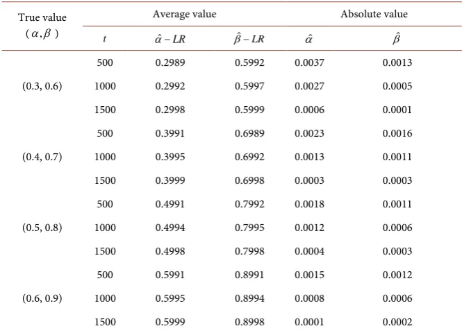
The simulation is based on (2.6) (2.7) and (2.12). First according to (2.6) and

(2.7), for given values of α β, and t such as α=0.3, 0.6β = and t=500,

we can get the sample values based on the likelihood ratio estimation and MATLAB. Then, for substituting the sample values into (2.12), the values of

( )

_{α βˆ,} ˆ _{can be obtained. Subsequently, we calculate the average values of the}

estimators. Finally, the average errors between estimators can also be calculated.

Simulation results are shown in Table 1. In Table 1, the time is represented as “t”

and likelihood ratio estimator is shown as “LR”. Table 1 lists the values of

“αˆ−LR“, “βˆ−LR “ and the average errors of “LR”. Table 1 illustrates that the

average errors of α β, depended on the size of given value of α β, . But under

the hypothesis of normal distribution, obvious difference can not be found

between estimators and true values, estimators are good. From the Table 1 we

can see clearly that the estimators become more and more close to the true value

by increasing the time t. The was of continuous time estimation is better than

the discrete observation [25]. (Those data comes from web of Statistical Data

and I use MATLAB to simulate those data to get the result. The confidence

intervals is

[

0.3 0.01, 0.3 0.01− +

]

for

α

=0.3,

[

0.6−0.01, 0.6+0.01

]

for

β

=

[image:12.595.206.539.89.329.2]

DOI: 10.4236/ojs.2017.76072 1050 Open Journal of Statistics Table 1. Likelihood ratio estimator simulation results of α β, .

True value (α β, )

Average value Absolute value

t αˆ−LR βˆ−LR αˆ _βˆ

500 0.2989 0.5992 0.0037 0.0013

(0.3, 0.6) 1000 0.2992 0.5997 0.0027 0.0005

1500 0.2998 0.5999 0.0006 0.0001

500 0.3991 0.6989 0.0023 0.0016

(0.4, 0.7) 1000 0.3995 0.6992 0.0013 0.0011

1500 0.3999 0.6998 0.0003 0.0003

500 0.4991 0.7992 0.0018 0.0011

(0.5, 0.8) 1000 0.4994 0.7995 0.0012 0.0006

1500 0.4998 0.7998 0.0004 0.0003

500 0.5991 0.8991 0.0015 0.0012

(0.6, 0.9) 1000 0.5995 0.8994 0.0008 0.0006

1500 0.5999 0.8998 0.0001 0.0002

5. Conclusion

In this paper, parameter estimation problem has been studied for the continuous time stochastic logistic diffusion model by using likelihood ratio. The explicit expressions for the estimation errors have been given and the according asymptotic properties have been proved by applying the he law of iterated logarithm, random time transformations, stationary distribution of solutions of stochastic differential equations and the law of large numbers for martingales. To get more accurate results, we use continuous observation method, and the proposed estimators are closer to the true value that be demonstrated by a simulation example. In the future research, we will consider the state estimation

problem for non-linear systems with incomplete observation [26] and

non-linear systems with random disturbance caused by Levy jump or Poisson jump [27].

References

[1] Makate, N. and Sattayatham, P. (2015) Stochastic Volatility Jump-Diffusion Model for Option Pricing. Journal of Huaiyin Teachers College, 01, 90-97.

[2] Lochstoer, L.A., Craine, R. and Syrtveit, K. (2000) Estimation of a Stochas-tic-Volatility Jump-Diffusion Model. Revista De Anlisis Econmico, 15, 61-87. [3] Intarasit, A. and Sattayatham, P. (2011) Option Pricing for a Jump Diffusion Model

with Fractional Stochastic Volatility. Journal of Nonlinear Analysis and Optimiza-tion, 11, 239-251.

[4] Roman-Roman, P. and Torres-Ruiz, F. (2012) Modelling Logistic Growth by a New Diffusion Process: Application to Biological Systems. Biosystems, 110, 9-21.

https://doi.org/10.1016/j.biosystems.2012.06.004

DOI: 10.4236/ojs.2017.76072 1051 Open Journal of Statistics of Metapopulation Dynamics. Ecological Modelling, 179, 533-550.

https://doi.org/10.1016/j.ecolmodel.2004.04.019

[6] Moller, J., Bergmann, K., Christiansen, L. and Madsen, H. (2012) Development of a Restricted State Space Stochastic Differential Equation Model for Bacterial Growth in Rich Media. Journal of Theoretical Biology, 305, 78-87.

https://doi.org/10.1016/j.jtbi.2012.04.015

[7] Knape, J. and De Valpine, P. (2012) Fitting Complex Population Models by Com-bining Particle Filters with Markov Chain Monte Carlo. Ecology, 93, 256.

https://doi.org/10.1890/11-0797.1

[8] Ji, L. (2016) Forecasting Petroleum Consumption in China: Comparison of Three Models. Journal-Energy Institute, 84, 34-37.

https://doi.org/10.1179/014426011X12901840102526

[9] Sakai, Y. (2008) Diffusion in Turbulent Pipe Flow Using a Stochastic Model.

Bulle-tin of the Jsme, 39, 667-675.

[10] Chen, J. and Chang, W. (1998) Modeling Differential Diffusion Effects in Turbulent Nonreacting/Reacting Jets with Stochastic Mixing Models. Combustion Science and

Technology, 133, 343-375. https://doi.org/10.1080/00102209808952039

[11] Pan, J., Gray, A., Greenhalgh, D. and Mao, X. (2014) Parameter Estimation for the Stochastic SIS Epidemic Model. Statistical Inference for Stochastic Processes, 17, 75-98. https://doi.org/10.1007/s11203-014-9091-8

[12] Xu, W. (2014) Parameter Estimation in Two-Type Continuous-State Branching Processes with Immigration. Statistics and Probability Letters, 91, 124-134.

https://doi.org/10.1016/j.spl.2014.04.021

[13] Zang, Q. (2016) Asymptotic Behaviour of Parametric Estimation for Nonstationary Reflected Ornstein? CUhlenbeck Processes. Journal of Mathematical Analysis and

Applications, 444, 839-851. https://doi.org/10.1016/j.jmaa.2016.06.067

[14] Zou, X. and Wang, K. (2014) Optimal Harvesting for a Stochastic Regime-Switching Logistic Diffusion System with Jumps. Nonlinear Analysis Hybrid Systems, 13, 32-44. https://doi.org/10.1016/j.nahs.2014.01.001

[15] Campillo, F., Joannides, M. and Larramendyvalverde, I. (2013) Estimation of the Parameters of a Stochastic Logistic Growth Model. Statistics, 1-30.

[16] Li, X. and Yin, G. (2016) Switching Diffusion Logistic Models Involving Singularly Perturbed Markov Chains: Weak Convergence and Stochastic Permanence.

Sto-chastic Analysis and Applications, 35, 364-389.

[17] Schurz, H. (2007) Modelling, Analysis and Discretization of Stochastic Logistic Eq-uations. International Journal of Numerical Analysis and Modeling, 4, 178-197. [18] Ovaskainen, O. (2001) The Quasistationary Distribution of the Stochastic Logistic

Model. Journal of Applied Probability, 38, 898-907.

https://doi.org/10.1017/S0021900200019112

[19] Pang, S., Deng, F. and Mao, X. (2008) Asymptotic Properties of Stochastic Popula-tion Dynamics. Dynamics of Continuous Discrete and Impulsive Systems Series A, 15, 603-620.

[20] Mao, X., Marion, G. and Renshaw, E. (2002) Environmental Brownian Noise Sup-presses Explosions in Population Dynamics. Stochastic Processes and Their

Appli-cations, 97, 95-110. https://doi.org/10.1016/S0304-4149(01)00126-0

[21] Brown, B.M. and Hewitt, J. (1975) Asymptotic Likelihood Theory for Diffusion Process. Journal of Applied Probability, 12, 228-238.

DOI: 10.4236/ojs.2017.76072 1052 Open Journal of Statistics [22] Peterson, A. (2014) Random Time Change with Some Applications. Auburn

Uni-versity, Auburn.

[23] Kailath, T. and Zakai, M. (1971) Absolute Continuity and Radon-Nikodym Deriva-tives for Certain Measures Relative to Wiener Measure. Annals of Mathematical

Statistics, 42, 130-140. https://doi.org/10.1214/aoms/1177693500

[24] Mao, X. (2008) Stochastic Differential Equations and Applications. 2nd Edition, Chichester, Horwood. https://doi.org/10.1533/9780857099402

[25] Liu, M. and Zhang, D. (2015) A Dynamic Logistic Model for Medical Resources Al-location in an Epidemic Control with Demand Forecast Updating. Journal of the

Operational Research Society,67, 841-852.https://doi.org/10.1057/jors.2015.105

[26] Sun, X. and Wang, Y. (2008) Stability Analysis of a Stochastic Logistic Model with Nonlinear Diffusion Term. Applied Mathematical Modelling, 32, 2067-2075.

https://doi.org/10.1016/j.apm.2007.07.012

[27] Liu, M., Deng, M. and Du, B. (2015) Analysis of a Stochastic Logistic Model with Diffusion. Applied Mathematics and Computation, 266, 169-182.