Computer simulation of river systems with hydro electric power stations

A report submitted in partial fulfilment of the

requirements for the degree of Master of Engineering,

at the Un.iversity of Canterbury, Christchurch,

Nm'l Zealand.

by

Bernard H··M. gBe,

:1.

ABSTRACT

This report describes the computer program "WASP" written

to test the feasibility of simulating a river

channel/lake/hydro-electric power-station system on a digital computer.

WASP is a progrruu package consisting of a main program

called CONTROL, and three principal subroutines: RIVER3 {models

open channels), JUNCTN {models channel bifurcations) and POND

(models flovlS through lakes and power-stations). To simulate

a river system using WASP, a user is required to write a new

sub-routine called SYSTEM, the statements of which consist of CALL

statements. Each of these CALL statements calls one or another

of RIVER3, JUNCTN or POND (the argument list referring to a·

particular part of the river system).

The CALL statements of subroutine SYSTEM describe the

architecture of the system.

At its present stage of development, WASP is capable of fast

and accurate simulat:.ion of open channels carrying stea.dy or slowly

fluctuating unsteady flows. Further vlork is required before :i.t

is able to satisfactorily simulate the wa·ter flow through a

ACKNOWLEDGEMENTS

I \'lish to express my appreciation of the assistance given

during 1::his study. In part:i.cular, I thank my supervisors Dr.

D.G. Elms, Dr. P.J. Moss and Professor I.R. Wood for their

guidance and assistance during the work. Also I thank Messrs

W. Fookes, J. Black, D. Goring,

s.

the Ministry of Works a.nd Messrs S. Astwood and D. Gorman of ·

the New Zealand Electricity Department for their time and effort

in providing essential information for the study,

For the production of this report I thank Drs D.G. Elms,

P.J. Moss and A.J. Sutherland for their comments on the drafts,

and Mrs. B. Stout for her patience \'lith the typing.

Bernard H-M. Gee,

iii

CONTENTS

PAGE

Abstract i

Acknowledgements ii

Contents iii

List of Figures and Tables v

Nomenclature vii

List of Symbols used in WASP diagram viii

1. HYDRODYNAMIC SIMULA'l'ION

1.1 Introduction 1

1.2 Formulation of the river system model 2

1.2.1 The Variables in a Model 4

1.2.2 Model Complexity 6

1.2.3 Program Efficiency 7

1.2.4 Experimental Design Features 7

1.2.5 Model Realism 8

2. A REVIEW O.E' SOME EXISTING OPEN CHANl\IEL FLOW PROGRAMS

2.1 Introduction 10

2.2 The Choice of a Language 12

2. 3 Existing Open Channel Flm'l Programs 13

2.3.1 The N.I.T. Unsteady Flow Computer Program 14

2.3.2 Program HYDRAC 15

2.3.3 Program ChNAL 16

3. DESCRIPTION OF THE CONFUTER PROGRAMS

3.1 Introduction 18

3.2 Choice of Algorithm 19

3. 3 Outline of the Ne·thod of Characteristics 21

3~4 RIVER2 22

3.5 RIVER4 25

3.6.1 Subroutine RIVER3

3.6.2 Subroutine JUNCTN

3.6.3 Subroutine POND

3.7 Simulating with WASP

3.8 The Problem with Meanders

3.8.1 Geometry and Flow Characteristics

3,8.2 Energy Losses

3.8.3 Numerical Considerations

3. 9 ·waterfalls, Rapids, Lateral Inflmv and Outflow

4. TEST CASES AND RESULTS

4.1 Introduction

4.2 Test Case for RIVER2 and RIVER4

4.3 Tes·t Cases for WASP

4.3.1 Test Case No. 1 for Subroutine

4.3.2 Test Case No. 2 for Subroutine

4.3.3 Test Case No. 3 for Subroutine

5. CONCLUSIONS AND RECOMMENDATIONS

5.1 Conclusions

5.1.1 General Conclusions for WASP

5.1.2 Limitations of WASP

JUNCTN and RIVER3

RIVER3

POND

5.2 Recommendations for further work on WASP

REFERENCES

BIBLIOGRAPHY

APPENDICES:

PAGE

29

29

32

34

36

36

38

39

41

42

43

46

46

50

52

56

56

57

59

61

64

A. Derivation of Ordinary Differential Equations for Unsteady Flow 67

B. Solution of Unsteady Flow Equation by the Method of Characteristics 70

c.

D. User's Manual for RIVER4 (inc. Listing)

76

Figure '1 2 3 4 5 6 7 8 9

10

c.

LIST OF FIGURES AND TABLES

Development Steps for a Simulation Model

Classification of Some Simulation Languages

Simplified Program Structure of CANAL

Decision Tree for Metl1ods of Solution

Macro Flow Chart for RIVER4

Rectangular Grid for Method of cr:_aracteristics

RIVER4 Hierarchy

The Concept of WASP

WASP Hierarchy

Rectangular Grid for Bifurcations

,JUNCTI.ON Macro !<'low Chart

POND Macro Flow Chart

Example of a Water Resource System

Meanders

Depth-:-Velocity Profiles

Ohio-Mississippi Junction

Water Surface Profiles for Test Case No. 1

Curve for Upstream Discharge

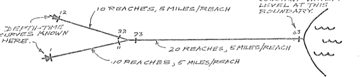
The Artificial River System

Cross Section through a Typical Hydry-Electric Power

Station

Water Level Curves

Control Volume for Unsteady Flow

c₁ and c₂ Characteristics

Rectangular Grid

+

-C and -C -Characteristics

WASP Hierarchy

An Allowable River System

Section Representation

v PAGE 3 12 16 20 23 24 25 26 27 29 31 33 34 37 45 48 49 51 52 53 54 67

70

.

73

78

79

Table

.c.4 Form of Input Data

c.S Definition of a Power-Station and Lake Variables

C.6 The System to be Simulated

C.7 Input Curves for Upstream Boundaries

C.S The Artificial River System

C.4.1 WASP-CONTROL Macro Flow Chart

D.l Section Representation

D.2 Form of Input Data

D.3 Channel Properties

1 Input and Output requirements for River System Models

2 Computer Times for Program Runs

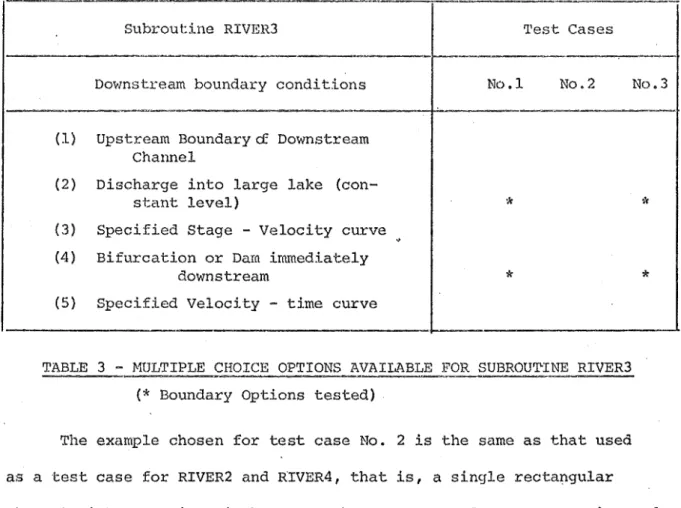
3 Multiple Choice Options Available for Subroutine RIVER3

c.l River Properties

C.2 River Properties

PAGE

82

92

96

97

98

104

115

116

120

5

44

51

97

NOMENCIJ\ 't'URE

CHANNEl~ SFTC/IONS (ARTIF/C::Irl/..1-Y .D/V/J;>f;i" THE CflAN/:1/.:::L INTO

R t-==A C II ES

J

Fig. {i) Elevation of Typical Channel

7 bed shear stress

0

S channel bed slope (angle a very small, i.e. cosd l)

0

SA'l:;:

t'SE'C:T/ON

A'RIEA.)

Fig. (ii) Typical Channel~

SHYR (section hydraulic radius) =

fix) Dx)

fit) DT)

reach length

simulation time increment SAR

p

values of depth and velocity at section P at time

=

YEP,VEP values of d~pth and velocity at section P at time

=

c+ positive characteristic

C negative characteristic

AI area at (same as SAR) section I.

NSC : number of channel section (usually t11e last downstream one).

g acceleration due to gravity

p liquid density

DEFINITION OF SYMBOLS USED IN WASP DIAGRAr--18

SYMBOJ_,

10 37

1 - - - - 1

1 >

-4'1

~8

IV-+'

DEFINITION

Represents a natural or artificial channel of a river system. This is modelled by subroutine RIVER3. The lower of the two numbers is the number of the upstream bound-ary section, whilst the other is the number of the dmvnstream boundary section.

Represents a channel bifurcation, and is

modelled by subroutine JUNCTN. Numbers are

boundary section numbers of channels forming

the bifurcation. The branches of the

bifurcation are in fact of negligible length, but have been drawn as such for clarity.

Represents an upstream boundary at \vhich the flow relationship is known and is available in RIVER3.

A downstream boundary at which the flow relationship is known and is available in RIVER3.

The open sea, in·to which the river empties. Water depth at section 96 is assumed to be constant throughout the simulation run.

Reservoir or lake with a single controlled ·

outlet. At least one inflow.

Hydro-electric power-station and reservoir with at least one inflow.

CHAPTER.I

HYDRODYNAHIC SIMUI,ATION

1.1 INTRODUCTION

Simulation is essentially a technique that involves setting

up a model of a real situation and then performing experiments on the

model, which is itself amenable to manipul~tions which would be

impossible, too expensive or impractical to perform on the entity it

portrays · (1) • This definition of simulation is extremely broad,

however, and may include seemingly unrelated things such as business

management games, physical models of major river basis,

econo-metric models and various electrical analog devices. Within the

context of this thesis, simulation will be treated as a numerical

technique for conducting experiments on a digital computer, which

involves certain types of mathematical and logical models that

describe the behaviour of a river system, over extended periods of

real time (1) •

Before any experiments can be conducted, a model of the x·iver

system must be constructed. In the past, many computer programs

which model unsteady flows in open channels have been v~itten.

Fewer have been written which model the water flow through the

pen-stocks, turbines and draft tubes of a hydro-electric power station,

but there appear to be none written which model the water flows through

a combination of both. As most systems with sizeable rivers in New

Zealand have at least one hydro-electric power station and consist of•

at least two or more reasonably large rivers (e.g. the Clutha, the

Waikato), there is a need for a computer simulation program which

is able to cater for a combination of rivers and powcr'stations.

In response to this need, three computer programs, RIVER2, RIVER4

and WASP, have been developed by the author. RIVER2, 'Jlhich models

unsteady flow in a single channel only, was written first·and was

used to test various mathematical procedures. RIVER4 is basically

a faster and more efficient version of RIVER2, and has in one case

reduced the computation time for a problem by eighty per cent of

that normally taken by RIVER2 for the sameprdblem. NASP is a

flex-ible simulation program which has been designed to model the water

flow through a river system composed of river channels1 lakes,

reservoirs. and hydro-electric power stations.

A more detailed description of >chese computer programs may

be found in Chapter III, whilst a user's manual and listings·may

be found in Appendices C and D respectively. Chapter IV discusses

the results obtained from running test case data on these programs,

and Chapter II reviews some of the computer programs written by

others to model parts of a river system, showing the limitations of

their prog:r:ams and how they have treated the difficulties inherent

in modelling a river system. The rest of this chapter is devoted

to a discussion of the formulation of the river system model,

esp-ecially the hydraulic principles involved, the mathematical techniques

used, the computer program layout and in general, the problems

involved \<Jhen modelling a river/lake/reservoir/power-station system.

1. 2 Formulation of the River System Model

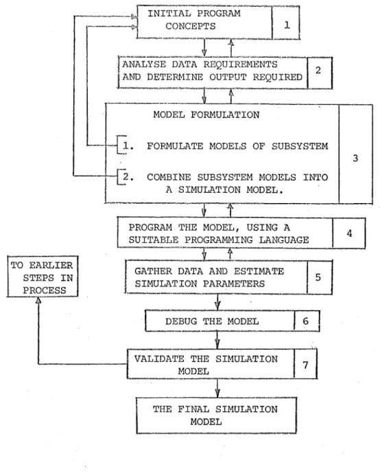
The development from initial concepts to the final computer

program model of a river system can often be traced through a series

of development steps, the number of identifiable steps and the

order in which they are carried out being highly dependent upon the

particular situation.

is shown in Figure 1.

points, the process

A flow chart of one such series of steps

Note that in this chart, at a number of given

returns to a previous step. That is, the

MODEL FORMULATION

FORMULATE HODELS OF SUBSYSTEM

~---r~ 2. COMBINE SUBSYSTEM MODELS INTO A SIMULATION MODEL.

PROGRAH 'rfiE MODEL, USING A SUITABLE PROGRAMMING LANGUAGE

TO EARLIER STEPS IN PROCESS

GATHER DATA AND ESTIMATE SIMULATION PARAMETERS

'---lrVALIDATE THE SIMULATION

L

THE FINAL

SIMULATI~N ~

MODEL

7

5

3

4

FIGURE 1 - DEVELOPMENT STEPS FOR A SIMULATION MODEL

five sections, the number of variables to be included in the model,

the complexity of the model, the computational efficiency of the

program, the amount of "realism" to be built into ·the model and the

compatibility of the models \'lith the type of experiments that are

going to be carried out with them; that is, ·the consideration of

the experimental design features that will be built into the models.

1.2.1 The Variables in a Model

One of the first considerations that enters in·to the .

formulation of a river system ~odel is the question of how many

variables are to be included in the model. Before this can be

done, the input and output requirements for the model.should be

determined. For a river system comprising river channels, river

bifurcations, lakes, reservoirs and power-stations, these are

different sets of requirements for each component of the system. For

example, a model which simulates a river will require as input data,

physical properties of the channel, initial flow conditions and water

behaviour over a selec·ted time period. On the other hand, a model

which simulates the \vater flow through a hydro-electric pov;er station

would require rating curves for penstocks, turbines, spillway sluice

gates and the like. (A complete summary of input and output

require-ments for a river system may be found in Table 1). Once these

requirements have been 'determined, then the nurnber of exogenous (or

independent or input) and the number of endogenous (or dependent or

output) variables can be finalised. For example, in a model of an

open channel, three necessary endogenous variables are the water

depth and velocity at points located along the line of the river, an

TABLE 1

INPUT AND OUTPUT ¥EQUI~MENTS FOR RIVER SYSTEM"MODELS

r---~r---·---.---·---~ Model

Components

River, canal or any other open flow channel.

Channel Junction

Lake or Reservoir

"Through-flow11

Power station with reservoir.

Input Requirements

1. Physical properties, in-cluding channel geometry.

2, Initial flow conditions.

3, Water flow behaviour over

a

{for channel boundaries).

1. Physical properties in-cluding channel geometry. 2. Initial flow conditions.

1. Physical properties in terms of volume-level curves.

2. The ratings of any inflow or outflow control struct-ures such as sluice gates, but excluding power

stations.

1. Physical properties in rel-ation to water flow

through the structure. Will be in the form of head loss-flow rate curves for penstocks, scroll ·tubes and rotating curves for spillway sluice gates and the like •

2. Initial flow conditions. 3. The behaviour of flow

through the station over a selected time period.

As for Lake & Reservoir and power stations with negligible storage.

Output Requirements

Water velocity and depth values at specified inter-vals along the channel.

Water veloQity and depth values at sections immediate-ly before the junction and at the section immed-iately after the junction.

Level and volume fluctuations, out-flow and inout-flow variations.

Flo\'/ rate 1 Head loss

variations, average electrical power produced.

Spillway flow

(it' any)

have been' fixed beforehand, then this particular endogenous

var-iable becomes a controllable exogenous·varvar-iable, that is a varvar-iable

or parameter that can be manipulated or controlled by the progran~er.

Non-controllable exogenous variables are generated by the

environ-ment in which the modeled system exists and not by the system itself.

Other endogenous variables may be the total flow past a point, the

average depth, or the deviation of the depth value at the point.

However, difficulty arises when determining the number of

exogenous variables, both controllable and uncontrollable, which

affect the endogenous variables. Too few exogenous variables may

lead to an inaccurate model, whereas too . many may make computer

simulation impossible because of an insufficient computer memory

capacity or may make computer programs unnecessarily complicated.

In models of hydro-electric power stations the latter may become a

problem, for most stations differ from each other and to allow for

these differences in a single computer program would be difficult,

Also, the consideration of things such as water hammer effects and

micro-second valve closings within the program may be necessary for

design and stress analysis purposes, but are superfluous in a program

which will model water flow over periods of days, months or years.

1.2.2 Model Complexity

The second aspect to be considered is the complexity of the

river system model. For such a model to be realistic, it must

necessarily be complicated in view of the large number of variables

and constraints inherent in any river system, and hence there is

the danger of constructing very complex programs which require an

unreasonable amount of computation time, regardless of how realistic

I

they may be. In general, any simulation program should be formulated

predictions about the behaviour of a given river system while

minim·-izing computation time. It should be tloted that the number of

variables in a model and its complexity are directly related to

computation time and validity, and altering any one of these

character-istics will result in an alteration of all the others. So in

7

the construction of a river simulation program some trade·~offs between these

characteristics will be inevitable.

1.2.3 Program Efficiency

This particular aspect is an important one, if simulation of

large river systems is to be a viable proposition. By program

efficiency or computational efficiency is meant the amount of

com--puter time required to achieve some specific numerical objective.

In relation to rj_ver system models, the main objective is the

min-imization of the amount of computer time required to generate values

of the endogenous variables over some specific time period being

simulated, such as six months or three years. Often this can be

achieved by employing a faster equation solving procedure to obtain

roots of polynomial equations, for example, in the first open channel

flow program developed by the author, replacement of the bisection

method for finding polynomial roots by the first order Newton

iter-ation procedure produced time savings of up to at least seventy per

cent. Other time savings may be made by storing oft-used values of

variables in the computer, instead of recalculating them for each

iteration loop.

1.2.4 Experimental Design Features

As these computer programs will be used in simulation

experi-ments, features should be built into them to allo>'l these experiments

example, to control water flow through a hydro-electric power station

either the turbines or spilhmys or both may be used. In this respect,

the section of the program that models a power station should have a

provision for varying spillway gate openings, the number of turbines

in the station and the flow through them. However, this means

com-plicating the program, and as stated in section 1.2.2, some

trade-offs will have to be made.

Before any simulation experiments can be run, the program has

to be validated; that is, all errors removed from it. 'l'his is

achieved by running the program on a set of data knotrm as a test case.

The correct output values for the test case are known, and for the

program to be error-free, its output and the known output values

should be identical. After the program has been validated, it ·

can'then be run on the data sets which constitute the .simulation

experiment.

1. 2.5 Realism

The remaining area of interest in model formulation is the

validity of the model or the amount of realism built into it. That

is, the adequacy of the model in describing the system of interest

or its accuracy in predicting the behaviour of the sys·tem in future

time periods. In models of a dynamic nature, such as a river system,

this realism is largely dependent upon the mathematical

representat-ions of the real-life situation. For unsteady open channel flow,

these mathematical representations are in ·the form of ordinary

differential equations. Their derivations however, were made on

the assumption that the water velocity was the same at all points

in any cross section of a river, an assumption trlhich simplified the

form of the differential equations (and hence made them easier to

solve), but \vhich introduces an error, as it is an approximation to

water-falls, tributary inflow and the like, must also be considered and

analysed to see if their inclusion or exclusion would seriously

affect the realism of the model. Difficulties arise when

attempt-ing to formulate a computer model of a power station, for realism

necessarily implies program complexity, which clashes with the need

to keep the program as simple as possible.

This conflict again emphasises the complete interdependence

of all the aspects of model formulation; that is, the nunwer of

variables to be included in the mocel, model complexity,

computat-:-ional efficiency of the program, the experimental compatibility of

the model and the model realism.

CHAPTER 'II

2.1 INTRODUCTION

After the river system model has been formulated, it then

has to be converted into a computer program. To do this a

program-ming or higher level language is normally used. One approach \.,rould

be to write the program for simulating a river system in one of the

\·;ell-known, general-purpose languages such as FOR"fRAN, ALGOL or IBM 1 _s PL/I. This offers the programmer maximum flexibility in :

(a) the design and formulation of the mathematical

model of the river system being studied;

(b) the type and format of output reports generated; and

(c) the kinds of simulation experiments carried out with

the model.

The principal shortcoming of this approach is the difficulty

encount-ered in writing simulated programs in a general purpose programming

language, for the sequencing of the interdependent actions forming the

model is often extremely complex and hence a major source of error.

Another approach \·muld be to use one of the simulation lan9uages

that are aimed at simplifying the task of writing simulation programs

for a variety of different types of models and systems. Among those

that have been developed within the last ten years are DYNAl.\10, CSMP,

GASPII, SIMSCRIP'r and GPSS (2). These languages have been developed

with the following objectives in mind ( 3 )

:-(a) to produce a generalised structure for designing

simulation models;

(b) to provide a rapid way of converting a simulation

model into a computer program;

simulation model that can be readily reflected

in the machine program;

(d) to provide a flexible way of obtaining useful

outputs for analysis; that is, outputs in a

relevant fo~-ma t.

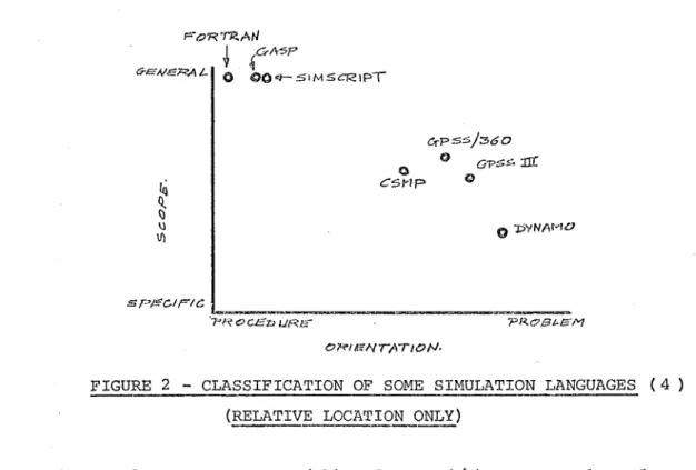
Most of these languages can be classified in terms of orientation

and scope or generality of application as in Figure 2.

Fo'RT'R.AN

.

*

G-E:N<EPAt. 0 OO<r-SIMSCRlPT

0

C~I'IP

erps:s}':360

O G'P5S. J!C

Q

FIGURE 2 -CLASSIFICATION OF SOME SIMULATION LANGUAGES (4)

(RELATIV~ LOCATION ONLY)

The two languages DYNAMO ( 2 ) and CSMP ( 4 ) are examples of

languages orientated towards models formulated in terms of non-linear

differential or difference equations, and variables that are

con-tinuous almost ever~~here in their range (some discontinuities can be

handled) are assumed. DYNAMO was originally developed for defining

models of business and CSMP for engineering design applications;

however, their applications could be interchanged. GASP and SIMSCRIPT

on the other hand, are very general, and both can do anything that can

be done in FORTRAN ( 4 ) • GASP differs from SIMSCRIPT in that the

former is not a complete language.

The simulation languages thus presented are only a fe>~ of the

many available and have been selected to shm"l' the wide spectra of

this.type of language, especially in relation to the more general

multipurpose ones such as FORTRAN or ALGOL.

2.2 THE CHOICE OF A LANGUAGE

As the simulation of river systems is mathematical in nature,

languages which are used for business data processing, such as COBOL,{5)

are automatically rejected because of their un.suitabili·ty. Also,

because of the inherent complexity of a river system.~ the choice is

further restricted to languages that are flexible and general in

application; that is, procedural rather than problem orientated,

excluding simu~ation languages which are orientated to a specific

type of problem.

In the final analysis, however, the decision whether to use a

particular language rests primarily on the following considerations

·-(i) the availability of the software, that is,

avail-ability on the desired computer;

(H) the availability of sufficient documentation;

(iii) the availability of programmers knm11ledgeable in

the particular language;

(iv) the necessary technical features, such as

trigonom-etric functions and the like, available in the

language. ·

Of the languages available on the Burroughs B6718 computer

of the University of Canterbury {ALGOL, FORTRAN IV, GASPII, DYNAMO,

SIMULA) at this time*, only FORTRAN IV and ALGOL satisfied all of

the four points previously mentioned. Of those two, FORTRAN IV

was selected by the author instead of ALGOL because of his greater

ing knmdedge of the former. Furtherrnore 1 in relation to river

systems, which are essentially dynamic in nature, specialist

languages (for example GASP) which cater for discrete event.systems

are automatically excluded.

FORTRAN IV consists of five major components: variables,

constants, subscripts, expressions and functions. The number of

different subroutines or functions available with this language is

limited only by the memory capacity of. the particular machine being

utilised. That is, the programmer has the flexibility of being

able to write almost any subroutine that he may need for a particular

simulation program, using a main program to call the specific

subroutinES when they are needed. For river/lake/reservoir/po\>ler

station systems, simulation programs. for each component of the

system \>Tould be written and combined into a single simulation program.

Needless to say, a modular approach of this type necessarily requires

that there be some degree of similarity in the basic structure of

the subprograms.

2.3 EXISTING OPEN CHANNEL FLOW PROGRAMS

To save programming time and to avoid possible duplication of

work, the author had considered modifying existing open channel flow

programs written by others.

examined on the basis of :

The programs selected by the author were

(i) the available documentation for the program;

(ii) the type of numerical procedures employed;

(iii) the simplicity of the program structure.

This last point is particularly important, for it means whether the

program can easily be altered or modified, or not. The choice in

section 2~2 of FORTRAN as a programming language placed little

written in ~ORTRAN. Of the six programs inspected (6), only three

v1ere found (RIVER, HYDRAC, CANAL) (6) that were suitable, in the

sense ·that they modeled unsteady flow in open channels. 'rhe structure,

tha·t is, the layout of the program ·logic, for two of the th:ree

programs was, on closer examination1 found to be extremely complex,

restricting alterations and modifications to very minor ones. The

third one of the group, on the other hand, had a relatively simple

s·tructure, but a limited sphere of application. This particular

program would have required extensive alteration to extend its sphere

of operations.

Thus, no suitable programs were found, although many useful

features of the programs were incorporated into RIVER2, RIVER4 and

WASP. A short review of RIVER, HYDRAC and CANAL appears in the

remaining portions of this chapter, showing why they were rejected

and any features which were utilised in RIVER2, RIVER4 and WASP.

2.3.1 The M.I.T. Unsteady Flow Computer Program (7)

This program was developed to determine "che characteristics of

flow· in open channels that resulted from hydro-electric power station

operation. To simulate open channel flow, RIVER (labelled as such

by the author for convenience) solves the differential flow equations

in Appendix A by the method of characteristics.

However, unlike the first order method detailed in Appendix B,

the method used in RIVER includes the second order terms in the

differential equations~ A large proportion of the complexity of

RIVER was due to this consideration of second order terms. Also,

unlike the other programs examined, RIVER has a complete documentation

which includes amongst other things, a derivation from first principles,

of the differential equations employed in the program.

computer runs by the author was that the programming language used

for RIVER was FORTRAN II, which is not a subset of FORTRAN IV, the

version of FORTRAN that is available on the Burroughs computer.

According to Sammett (8), FORTRAN IV is not a compatible extension

of FORTRAN II, but a new creation. To adapt RIVER to the Burroughs

computer would, therefore, require rewriting of the program.

Two features, or aspects, of this program were utilised in the

data input segments of RIVER2 and RIVER4. The first is the provision

tha·t the program has for handling irregular sec·tion geometry as well

as regular. RIVER has achieved this by requiring section tables

describing cross sectional area, hydraulic radius and water surface

width for a series of water depths for each section (refer to

nomen-clature) to be read in as part of the input data. '!'his provision

means that the program is flexible, but at the expense of input data

simplicity. The other feature is a linear int:erpolation routine for

the section tables; that is, if the properties of a channel vary

linearly, then only the tables for the end section need to be read

in, for the program interplates for the intermediate sections.

2.3.2 ~ogram HYDRAC

Written by A.G. Barnett of e1e Systems Laboratory of the Ministry

of Works, HYDRAC was designed to solve unsteady subcritical flows in

trapezoidal canals. Two alternative channel layouts are available

in this program, either a single channel with varying discharges

specified at each end, or a bifurcating system of three canals with

varying discharges specified at the three unconnected ends. The

finite difference scheme was used in HYDRAC and is an extension of

Barnett's previous work on rectangular channels (9), which is itself

an extension of the Richtmyer method (10). Bifurcation problems are

solved by a modified form of the method formulated in Stoker {11).

This program compiled and ran successfully on the Burroughs

computer, but the absence of any documentation save on input data

description, together with the intricate program structure, prevented

any detailed examination of it, and hence any modifications thereof.

For these reasons HYDRAC was shelved.

2.3.3 Program CANAL

Obtained from Mr G. Harris of Australia, this program solves

unsteady supercritical and subcritical flows in open channels, by

the method of characteristics as outlined in Streeter and Wylie (12).

CANAL (labelled as such by the author for convenience) , is restricted

to single channels of constant rectangular or trapezoidal cr~ss section.

The most notable aspect of this program was the simple, logical layout

of the program structure (see Fig. 3). This particular feature allowed

an easy understanding of the program, despite the fact that there was

very little documentation of the program.

1 INPUT DATA

r--CALCULATE MIN. VALUE OF 1 2

+I*

v AND TIME STEP DT

3 CALCULATE +VE CHARACTERISTIC

4 CALCULATE -ve CHARACTERISTIC (INC.

CHECK FOR SUPER OR SUBCRITICAL FLOW)

-

-5 OUTPUT VALUES

-6 CHECK IF SIMULATION OVER.

GO TO STEP 2 IF NOT

7 FINISH

The layout of CANAL has been incorporated into the RIVER2,

RIVER4 and WASP programs. A predominance of programming errors,

plus the absence of sufficient documentation prevented any

success-ful computer runs with CANAL.

CHAPTER III

DESCRIPTION OF THE COMPUTER PROGRAMS

3.1 INTRODUCTION

This chapter describes the computer program WASP writ·ten to test

the feasibility of simulating a river system with hydro-electric power

stations, on a digital computer. The main purpose of this program

would be to allow the user to model the flo~ pattern of a chosen system and then to appraise the effects of altering the flow pattern (e.g. by

building a hydro-electric power station across a river, increasing the

channel width, etc.) without resorting to hydraulic models or.to

experiments on the actual system itself.

A cursory ·examination o~ river systems by the author, indicated

that most of them could be viewed as a composition of natural or

artificial channels, lakes and hydro-eelectric power-stations; that

is 1 each system could be broken down into basic elemen·ts or components

common to each other. From another viewpoint, this means that providing

sufficient numbers of each of the components were available, any river

system, within reason, could be built. Designed along these lines,

WASP provides (that is, in relation to computer simulation of river

systems), the basic components in the form of three main subroutines:

RIVER3 {models unsteady flow in an open channel), JUNC'I'N (models flow

through a channel bifurcation) and POND (models the flow through a.

power-station with a storage reservoir or a lake with a controlled outlet,)

WASP itself is basically in four parts: CONTROL (main program)

and subroutines RIVER3, JUNCTN and POND. CONTROL is the key part,

for it runs the simulation of a river system; that is, it reads in

the values of the exogenous variables and the initial conditions,

starts the simulation clock, runs the system model (built up from _I

RIVER3, JUNCTN and POND), prints out the values of the endogenous

variables and stops the simulation when the allowable time limit is

In the centre portion of th:i.s chapter the four parts of WASP are

detailed, together vdth a description of how they have been combined

to form WASP. The description of two other computer programs (RIVER2

and RIVER4) which were the forerunners of subroutine RIVER3, toget.her

with an explanation of the numerical method used to model unsteady

flow in open channels 1 appears in earlier sec·tions.

Other aspects of river systems such as rapids, waterfalls, river

meanders and tributary inflov1, all of which have been tacitly ignored

in the fonaulation of the programs, will be considered further on

in the chapter.

3.2 CHOICE ALGORITHM

Of the many mathematical methods available for solving the

partial differential flow equations, two are particulaJ;ly suitable for

use on a digital computer. These are

:-(i) the method of characteristics; and

(ii) the Implicit method.

The latter method requires the differential equations to the

trans-formed into the corresonding finite difference equations. These are

then solved by setting up as many equations as there are unknown

dependent variables and then solving them simultaneously. That is,

if a channel is divided into five reaches each DX long, then the unknown

dependent variables are the values of depth and velocity at time T + 6t

at each of the six sections along the channel. With the aid of a

.digital computer, ·the resulting twelve equations could be solved by

iteration. For a large number of sections~ the computations involved

become tedious. However, the restriction on 6t as encountered in the

method of characteristics (Courant condition) is removed and larger

values of 6t help to compensate for the tedious iteration. A more

detailed description of this method may be found in Ref. 13.

The method of characteristics is a well documented method and is

popular because it gives results with a reasonably high order of

accuracy in return for relatively easy programming. The only

drmV'-back that has been found with this method is the large amount of

computer time required by the simulation program whenever lengthy

real-time periods are simulated.

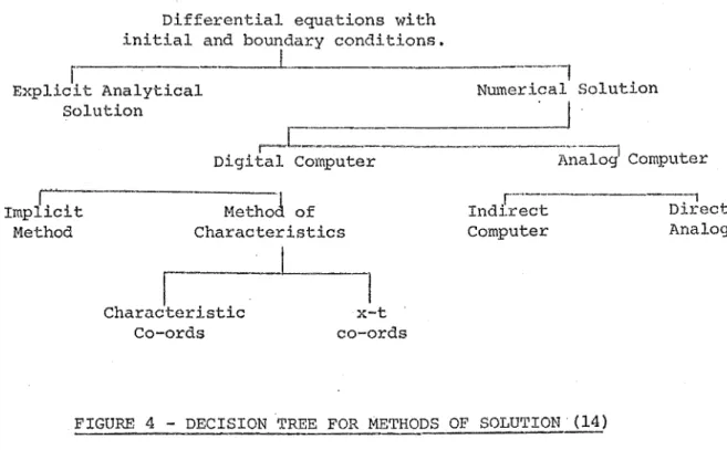
Because of the tedious computation involved with the Implicit

method and because of the extensive documentation on the method of

characteristics and a dearth of literature on the Implicit me.thod,

the method of characteristics was chosen instead of the Implicit

method. The decision tree in Fig. 4 presents these two algorithms

in relation to other procedures.

r

Differential equations with initial and boundary conditions.

Explicit Analytical Solution

---,

Nmnerical Solution

Computer Computer

I ..

Method

MethoJ of Characteristics

1....

.

l

x-t Characteristic

Co-ords co-ords

FIGURE 4 - DECISION TREE FOR METHODS OF SOLUTION (14)

;-1

D~rect

3. 3 OUTLINE OF THE METHOD OF CHARACTERIS'riCS

''l'he solution of steady flow in an open channel may be obtained

by the use of a combination of ·the specific energy, momentum,

continuity and Manning equations, depending on·whether the flow is

uniform or non-uniform. In the case of unsteady flow, the first

two equations cannot be used due to the assumption made during their

derivation (steady flow assumed). Therefore in trea·ting unsteady

flows it becomes necessary to reconsider the equations of motion in

relation to this type of flmV".

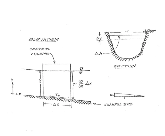
By considering a control volume of a channel with bed slope S₀

and constant shear stress T on the bottom sides, two partial diff-o

erential equations for unsteady open channel flow are obtained. These 21

two equations are transformed into the ordinary differential equations (1)

by the method of charac·teristics (Appendix A)

where A dx dt

L

=

=

.,... - + dv

dt

+~

- A I A

A dy + !.Q. -gs =

dt pR 0

=

0

...

=

To solve equations (1) a numerical step me·thod (involving finite

differences) together with initial conditions and boundary conditions

is used. Appendix B contains a derivation of the finite difference

equations from equatiorts (1) and details the solution procedure for

each of the two basic finite difference grids. For the programs

RIVER2 , RIVER4 , RIVER3 , (the latter being a WASP subroutine) 1 a

rectangular grid or net is employed in preference to a characteristic

grid. The use of a rectangular grid enables depth and velocity data

for all river sections to be calculated and printed out at one time

instead of irregular times as would be the case for a charac·teristic

3.4 RIVER2

This program was originally developed in the absence of other

suitable open channel flow programs {Chapter 2) and was later used as

a 11_{test bed}11 _{for new numerical procedures before their insertion into}

WASP. Basically, its formulation follows the mathematical procedure

outlined in Appendix B. The rest of this section is devoted to an

outline of the program structure and operation.

Referring to the macro-flow diagram (Fig.5), the main program

initially reads in the simulation ti·tle; simulation control data,

channel properties, initial conditions and boundary conditions. All

this data is then echo-·printed. The data for RIVER2 (and RIVER4)

differs from the subroutine RIVER3 of WASP in that there are no

provisions for S.I. units, and that only one value of Manning's n

for the whole channel is catered for.

The simulation time clock is then initialised and subroutine

THETA is called. This subroutine calculates the maximum time

incre-ment allowable under the Courant condition; and then sets the actual

time incremen·t to be 99% of this, i.e.

:-TH

=

Subroutine INPOL2 is used by THETA to calculate AN and TN from the

section tables. This is accomplished by a linear interpolation

between the table entries.

Next the new values of velocity and depth VE & YE) at all the

internal grid points (i.e. all sections except the upstream and

down-stream boundaries) are calculated from the previous values (VI & YI)

INPUT ';DATA. FCI+o-Pi<!Nl·

J~o

_,.

A/..'-~-- \iwy:~~$

/

I

[;;hu '"

I

I

I

...

l

l

·I

23

I

_Fl-:"':l·

: C/I·LCU)..ATI:i-

J

C:::At...c]~-A~-~-·1

I

I PaR :S~H3cg IT't cAL.. I'"' l-0\1/ FDH ~UPer-:..c~·.<<fTICAL. p:v_;\,J

I

l'*---·---~----~-1 I

I . CA!..C:Ul-AIE:

I

I

I

y~3-l----~~L_

No

C-AI:.cu l-IITE

NEJI:j--:r>EP'Tif AND

VEhC'c:: IT'( V/\I.UE.5

FOF~ UP>Tt<.DAf\11

AN'D :PPWNS'fRE:AM

'f?,ouNJ;>AR..'/

=:-r-3cnoNS • _ J

PR~·iJfcncr

1.1-J

ltMfi

.6t

1

-A B

/fi\

(""f:.~NCL~

2 3 J;- '5 ~ .• ·- NSC·-1 NSC,

UPS"/7'!/E:AN E""lJMZ:!Al<V. ::Dt?W/'/5/RC~AI'-1

Z>fEPTN AND VSLOC.I/f BoUN:l.)AR'(.

/<NOkiN ALON<r Nf;:'RfE'.

/V.l?f N:5c X:S -niE NUNB!ER <!?P IHE

X>O t:.l# :S?7<ei\M 13 OIJNPAR'/ SEC/loll/.

FIG.6 - RECTANGULAR GRID FOR METHOD OF CHARACTERISTICS

For each point P in Fig. 6, the values of VIR and YIR are

calculated first by the subroutines RPCHIC and SLOPE (see Fig. 5 ) •

A check is then made by the program to decide whether the flow at the

section is super or subcritical. Depending on the outcome of

this check either VI

8 and YI8 or VIs' and Yis' are calculated by

subroutines RNCHIC (suitably modified) and SLOPE. Finally, using

equations (5) and (7) in Appendix A, the values of VEP and YEP are

extracted.

The remaining dept.h and velocity values to be calculated are

those of the upstream and downstream boundaries. In RIVER2 the

values of depth and velocity at the upstream botmdary are known at

all times along the time axis {Fig. 6), paired values of depth and

velocity at specified time intervals having been read in as part of

the input data. The values of YE and VE are linearly interpolated

0 0

from these paired values of depth and velocity.

At the downstream end, no problems are encountered when the

flow is either super or sub-critical. Equations (7) and (8) in

I

25

used to obtain YENSC and VENsc' When all the paired values (YE₁,vE₁),

(YE₂,VE₂), ••••• (YENSC'VENSC) 1 (see Fig. 6) have been calculated, they

are printed out by the program, which afterwards resets the YE and VE

values as the new YI and VI values.

Lastly, the simulation time clock is checked against the total

time allowed (TTIME) and if 'rTIM.E is exceeded, the simulation run is

terminated, otherwise the procedure outlined above is repeated.

FIGURE 7 - RIVER4 HIERARCHY

3.5 RIVER4

This program is identical to RIVER2 except that in subroutine

CHIC has been replaced by subroutine CHIC2. CHIC uses the method of

bisection to solve for values of VIR and YIR whilst CHIC2 uses the

faster Newton iteration procedure. A listing of RIVER4 may be found

in Appendix D together with a user's guide.

3.6 WASP

Program WASP (an acronym derived from "Water Activity Simulation

modelling the flows through the hydro-electric power-stations and

doi-m the river channels; it consists of four main parts, CON'l'ROL

(main progrant) and three subroutines: RIVER3, JUNCTN and POND. To

simulate a river system, the user first writes a new subroutine SYSTEM

using the three subroutines (RIVER3, JUNCTN and POND) to describe the

system; that is, these subroutines are used as "building blocks" to

construct the river system. 'rhis relationship is shown in :b,ig. 8.

The inter-relationships between the V'lASP subroutines are shown in Fig .10.

§upplied by WASP

I

(main program)

Reads in data required for simulations.

Activates the simulation run by calling

sub-routine SYSTEM. Prints out results Terminates the simulation

n~-~r-·---~~

~:.:_:~'?_~~~nes)

j

Programmer written

'

'"""-=-"""'"---=--

· ~ (subroutine written by

user).

Calls a combina·tion of

, __ Ju~~~nd ~~

8 - THE CONCEPT OF WASP

Simulation control data, pmv-er station and channel properties,

·initial conditions and channel boundary conditions are read in and

echo-printed by CONTROL. This part of WASP then activate~ the

simulation run by calling subroutine THETA (same as that in RIVER2)

to calcula·t:e the time increment t:.t. Next, the programmer-written

· subroutine SYSTEM is activated and the \vhole network is taken through

27

\Q

lf\

.}

1--li)

1!.

.j

'I

-I

~

UJ

-l

\)

~

\l

(J

~

{),.

~

Q

~

<.

~

~

h

l-t

N

M

~~

Li

·

~

[__-~-·-:~

0

~

:t.

\j

---(YE

1,vE1), ... (YENSC'VENSC}, together with collated statistics

from each power station are printed out by CONTROL, which then

resets the YE and VE values as the new YI and VI values. Finally

as in RIVER2 the simulation time clock is checked against the total

time allocated (TTIME} and if the cumulative time is less than TTIME,

the whole procedure is repeated, otherwise the simulation run is

terminated.

Fig. 9 shows ·the WASP hierarchy, the rest of the section

contains a description of the three basic subroutines, and a detailed

description of WASP may be found in Appendix

c.

3 • 6 .1 Sub-routine RIVER3

This subroutine is a modified version o£ RIVER4 in that

only subcritical flow is allowed for (due to the limitation imposed

by subroutine JUNCTN}, and that all the data that it requires is

read in by CONTROL. Also, there is a multiple choice of both

downstream and upstream boundary conditions, ranging from specified

velocity-depth input values,.to discharge into a large volume of water

(static water level). If RIVER3 encounters supercr:i.tical flow, an

error message is printed and the simulation is stopped. subroutine

RIVER3 differs from RIVER2 in the same manner that RIVER4 differs

from RIVER2 that is, the replacement of CHIC by CHIC2 (Fig. 9 ).

3.6.2 Sub--routine JUNCTN

This subroutine has been "~:v'ritten to solve the equations

associated with two channels (not necessarily the same) meeting to

form a third. As inferred in section 3.6.1, only subcritical flow

has been provided for. It has been assumed that both upstream

branches of the junction are subcritical and that the joining of

these· two flO\'lS produces a third subcritical flow - tlfis assumption

is reasonable if

29

downstream of the junction is approximately equal

to the sum of the cross-sectional areas immediately

upstream of the junction;

(b) the flow 'in both upstream channels is well into the

subcritical range;

(c) the included angle between the two joining channels

is small.

JUNCTN solves the bifurcation equations formulated in

Stoker (16) by the 1st order Newton i·teration procedure.

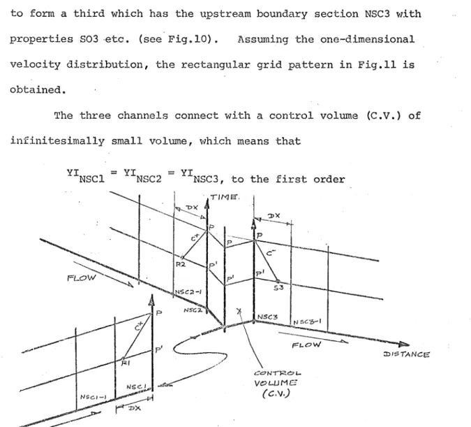
A Brief Description of the Formulation:

Consider two channels with downstream boundary sections NSCl

and NSC2, and with properties SOl, S02 (reach slopes) etc. joining

to form a third which has the upstream boundary section NSC3 -v1ith

properties S03 ·etc. (see Fig.lO). Assuming the one-dimensional

velocity distribution, the rectangular grid pattern in Fig.ll is

obtained.

The three channels connect with a control volume (C.V.) of

infinitesimally small volume, 'Vlhich means that

YINSCl = YINSC2

=

Solving for YIRl' VIRl' YIR_{2, VIR2 , YI83 , VI83 by the 1st order}

Newton iteration procedure and by substituting in equations

(5) and (7) in Appendix B, three equations (one for each branch) in

four unknowns (VENSCl' VENSC_{2 ,} VENSCJ' YENSCl = YENSC₂ = YENSCJ) are

obtained.

= VINSCl -

·;g

•rRI

ARI (YENSCl -YIR1)-g(SF1- SOl) ~t ·

...

VENSC2 = VINSC2 - _AR2 TR2 (YENSC₂ -YIR₂) -g (SE'2 - S02) ·~t (3)

VE

=

+

I

NSC3 NSC3 AS3 (YENSCJ -YIS3) -g (SF3- S03) ~t .•• (4)

where SOl, S02, S03 are the bed slopes of reaches 1, 2 and 3, SFl,

SF2, SF3 are the friction slopes calculated from Nanning's equation

by SLOPE, and TRl, ARl, TR2, etc. are the top widths and section areas

corresponding to YIRl' YIR

2, YI83• volume gives the fourt~ equation

:-Applying continuity to the control

FN - VINSCl Al

+

+

where Al, A2 and A3 are the section areas calculated by INPOL2 for YE

at NSCl, NSC2 and NSC3 respectively. The value of YE 'is obtained by

the procedure outlined in Fig. 11.

If the flow is unsteady, then the values of YENSCl' VENsel'

VENSC 2 , and VENSCJ will not be the same as YINSCl' VINSCl, VINSCZ'

and VINSCJ" Hence the procedure uses the method of bisection to

find YP. As FN is a function of YP, it is used as an indicator for

when the correct value of YP is obtained (i.e. when FN

=

Problems arise when supercritical flow is present in the

channels. For example, in the calculation of YIS

3and

vr

indicated in Appendix B, the point S3 moves upstream for supercritical

NIE' W CDE?TH ,·s

G"I"TI-/JE'J< VTKA_,>'.J'J(B

01< Y./J<c. CALC111..AIE:

/VF-'h/ VF-/-OC 17/l-i:S.

y ?'__. y P -"< _, 'l.T I<A .)

YTI<EJ../ Y:TI<C. J FNA..~

FNB All.l">FIVC ARe·

"DLJMf1Y VAT,...1Al3L€$.

: YTI<A = YPX

YYKB ""(YP+Y?X)/.Z

""'yr

L

---t-=1>/A-= PN (y:r KA) rNB"'-;t=N (YJJ:J3) t=/V C =rtl fJ<C

31

SET-'

NO Y.T..CCA "' YJ!<A

Y::rJ<c""" Y.r.KB Y..7f.<B "'(Yfi<Ar

---]

Se:T:

'J::n<A""' Y:n<B · Y:rt<c~ Y.7k8'

present, there has been lit·tle accomplished concerning the

converg-ence ·of two supercritical flows, or of one supercr:i.tical and one

subcritical. For this reason, WASP has been restricted to

sub-critical channel flows.

3.6.3 Subroutine POND

Subroutine POND was originally written to simulate the water

flow through a po;qer station and reservoir; but later was expanded

to cope with

a lake or reservoir which has no power station associated with it, but

which has a controlled outflow.

For the power station and reservoir option, the following

-· procedure calculates the approximate water flow through the station.

(a) Initially, the nett inflow into the reservoir over

time period At is calculated. This inflow produces

an increase in lake level.

(b) Subroutine I~WOL3 calculates the allowed flow rate

·through the turbines (and therefore the total flow

over At), and together with any spillway flow, the

total outflow from the reservoir for At is obtained.

However, the effective or nett head changes as the

lake level changes, so the new reservoir level is

taken as an-average of the level calculated in (a)

and the final level. The difference beb.reen this

level and the level of the previous time step is

printed out as a reservoir storage or deficit depending

on the sign.

(c) Finally, values of depth and velocity at the downstream

sections of inflowing rivers and at the upstream section

of outflowing rivers (from the stilling basin) are

8

_r

CALC:UL/+TL--

TOTAL-1/VF.Lotv p·o7c.: 'PI"Er-:.lo.D .b.·t, A N:D /VF!W LAkE OR

R.E 5 r::·1-? V..-:71:~ L

.:c;·

2

TW<BINP-G.

C /\-/.... C i.J/....AT/3' · o urr-= L-OW 7HP,.c.?UC:.H GA7'l~o·.s.

CA LCUL/\IE! SIC':RACTE:::

IN LAI<E' 0~ 7<. L!.SEi" VOIR.

c

c u

LJ P".-c:. "7""T: r: AM AN b

:DOW!VSTR IEAt1 RIV!E'R

B auNt::> A "RI e: .s.

33

NGO::/: POWcR-5/ATJON

W!TJ-} RE5£ERVOIR.

NG-0:: '2: LA!<~ W lrJi

Co~OLI-F-'.:D OUTJ. .. P-7:

The lake-only option uses half of the first optioni the

power-station section being side-stepped by the program.

The whole POND subroutine is an attempt ·to produce a program

which is not merely a water level-power outpu·t relationship, nor a

complicated mathematical procedure involving micro-second valve

closing times and water hammer effects, but a compromise between the

two types. Naturally, wa·ter hammer effects and valve closing times

are essential for design purposes1 but not so for a simulation program

involving time periods of days. A macro-flow diagram of POND is

presented in Figure 12.

3,7 SIMULATING WITH WASP

As indicated beforehand, the progrrumaer is required to write

subroutine SYSTEM by using the three "building block" subroutines

supplied by WASP, to simulate the desired water resource system.

For example, consider the following system (E'ig .13 ) of two j1.mctions,

seven stretches of channel, one power-station and reservoir, and

one lake with a controlled outflow.

.PoWt::R :5TATICIN -r 7<ESEi"F-<:~t:?l.~ •

FIGURE 13 - EXAMPLE OF A WATER

CCNST,ANT ,5-r/Jo·c

.:5ro~A GG!'

Where R7 enters the sea, the stage has been assumed to be constant

because of the negligible effect of the river discharge upon the

sea level.

For this system, subroutine SYSTEM woul~ be as follows:

(FORTRAN IV) :

SUBROUTINE SYSTEM

35

CALL RIVER3 (argument list) + with correct options for boundaries of Rl

CALL RIVER3 +with correct options for boundaries of R2

CALL JUNCTN (boundary· sections of Rl, R2 and R4) + for Jl

CALL RIVER3 ( - - - ) +ditto for R3

CALL RIVER3 ( - - - - ) · ~- ditto for R4 CALL JUNCTN

CALL RIVER3

C---~--- R3, R4 & R5) + for J2

+ ditto for R5

CALL POND (Reservoir and Power station option) + for Pl

CALL RIVER3 + ditto for R6

only) +.for P2

+ ditto for· R7 CALL POND ( Reservoir

CALL RIVER3

RE'fURN

END

The data which 'Vlould have to be read in for a simulation run

for the above system would be as follows: (in addition to the control

data) :

1 .. Section geometry· for all sections in Rl to R7

2. Initial conditions at all sections in Rl to R7.

3. Section geometry and initial conditions for Jl and J2.

4. Rating curves for the peustocks, turbines, generators,

spill-way gates and tailwater level for Pl.

5. Reservoir level rating curve for Pl and P2.

6. Initial turbine flow rate for· P:t

level for Pl and P2.

7. Pai~ed values of depth-velocity against time or depth

against time for the upstrem boundaries of Rl, R2 and R3,

8. Discharge-time values for turbine flo\'l for Pl.

A detailed exa~ple of a simple water system showing input data and output values may be found in Appendix

c.

3.8 THE PROBLEM OF MEANDERS

Throughout the formulation of RIVER4 (and RIVER3), the effects

of a channel bend upon the water flO\v had been tacitly ignored. In

this section some of these effects are examined: their nature, the

extent of their influence and possible numerical representation.

3.8.1 Geometry and Flow Characteri~ics

The most characteristic features of all natural channels (and

some artificial ones), regardless of size, is the absence of long

straight reaches and the presence of frequent sinuous reversals of

curvature (15), which are comrnonly knm-m as river bends or meanders. (Strictly speaking the name meander is usually associated vlith river

bends which exhibit regular reversals as well as an overall path

symmetry). A statistical study by Leopold and Wolman (16) showed

that bends tended to be scaled versions of a given set of proportions,

that is, large rivers tended to have large bends and small rivers to

have small bends. An interesting aspect of this trend is that most

rivers tend to look similar on planimetric maps due to the ratio

of curvature to width (rw/w} for these rivers being close to each other.

Fig. 15b shows three examples in which the scales have been chosen such

that meander length is equal on the page.

A cross-section of a typical meander at A-A (Fig. 15c) would

show an asymmetrical shape which would be deepest near the concave