An analysis and study of decision tree
induction operating under adaptive mode to
enhance accuracy and uptime in a dataset
introduced to spontaneous variation in data
attributes
Uttam ChauhanDepartment of Information Technology,Charotar University of Science and Technology, Changa Amit Ganatra, Amit Thakkar & Yogeshwar P.Kosta
Charotar University of Science and Technology, Changa
ABSTRACT
Many methods exist for the purpose of classification of an unknown dataset. Decision tree induction is one of the well-known methods for classification. Decision tree method operates under two different modes: non-adaptive and non-adaptive mode. The non non-adaptive mode of operation is applied when the data set is completely mature and available or the data set is static and their will be no changes in dataset attributes. However when the dataset is likely to have changes in the values and attributes leading to fluctuation i.e., monthly, quarterly or annually, then under the circumstances decision tree method operating under adaptive mode needs to be applied, as the conventional non-adaptive method fails, as it needs to be applied once again starting from scratch on the augmented dataset. This makes things expensive in terms of time and space. Sometimes attributes are added into the dataset, at the same time number of records also increases. This paper mainly studies the behavioral aspects of classification model particularly, when number of attribute in dataset increase due to spontaneous changes in the value(s)/attribute(s). Our investigative studies have shown that accuracy of decision tree model can be maintained when number of attributes including class increase in dataset which increases the number of records as well. In addition, accuracy also can be maintained when number of values increase in class attribute of dataset. The way Adaptive mode decision tree method operates is that it reads data instance by instance and incorporates the same through absorption to the said model; update the model according to value of attribute particular and specific to the instance. As the time required to updating decision tree can be less than introducing it from scratch, thus eliminating the problem of introducing decision tree repeatedly from scratch and at the same time gaining upon memory and time.
Keywords: decision tree induction, classification
1. Introduction
predefined accuracy is achieved, model can be used to derive unknown values. The problem of this approach is that once decision tree classification model is built up, than it cannot be modified for some new instances though they are related with the dataset. Since the aim behind including new instances is to achieve better classification model, those instances to must combined with existing instances and then decision tree classification model can be derived from scratch. There might be the case that training data set is too large to fit in main memory. The method should be able to eliminate the constraint of space.
2. Modes of Decision tree induction
An approach in which the decision tree classification model is derived from fixed set of training instances and cannot be updated is called non-adaptive mode of decision tree induction. The existing decision tree induction method is based on non-adaptive mode. A non-adaptive mode is appropriate for learning task in which a single fixed set or training set is provided. But it is not possible that a dataset, on which the decision tree has been inducted, remains static forever. Data are generated periodically and needs to be considered. This would lead to approach that provides facility to update or restructure existing model for new data instances. The cost of inducting tree from scratch may be too expensive to apply a non-adaptive method to serial learning task. Using adaptive approach, new decision tree can be inducted based on data set and existing decision tree can be updated as well.
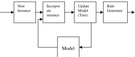
Figure 1. bBlock diagram for adaptive mode of decision tree induction
2.1. Gain ratio calculation
In to the process of decision tree induction, at every test node, there would be some test attribute based on which whole dataset is partitioned repeatedly. There would be a question that which attribute is to be select as test attribute. There are several attribute selection measure exists like information gain, gain ratio etc. can be used to select test attribute at the particular node. Information gain is one of the widely used methods for attribute selection, but it bias towards the number of distinct values in the attribute.[ Chawla] Gain ratio is the measure which eliminates this limitation. The procedure for calculating gain ratio is described here. The gain ratio measure is used to select the test attribute at each node in the tree. Such a measure is referred to as an attribute selection measure or a measure of the goodness of split. The attribute with the highest gain ratio (or greatest entropy reduction) is chosen as the test attribute for the current node. This attribute minimizes the information needed to classify the samples in the resulting partitions and reflects the least randomness or impurity in these partitions. Such an information-theoretic approach minimizes the expected number of tests needed to classify an object and guarantees that a simple (but not necessarily the simplest) tree is found. Let S be a set consisting of s data samples. Suppose the class label attribute has m distinct values defining m distinct classes, Ci (for i = 1; : : :;m). Let si be the number of samples of S in class Ci. The expected information needed to classify a given sample is given by:
mi i i
m
P
P
S
S
S
I
(
1,
2,...,
)
1log
2
(
)
(1)
where pi is the probability than an arbitrary sample belongs to class Ci and is estimated by si/s. Note that a log function to the base 2 is used since the information is encoded in bits.
Let attribute A have v distinct values, {a1, a2,av}. Attribute A can be used to partition S into v subsets, {S1, S2,
Sv}, where Sj contains those samples in S that have value a j
of A. If A were selected as the test attribute (i.e., best attribute for splitting), then these subsets would correspond to the branches grown from the node
New Instance
Incorpor ate instance
Update Model (Tree)
Rule Generator
containing the set S. Let sij be the number of samples of class Ci in a subset Sj . The entropy, or expected information based on the partitioning into subsets by A is given by:
)
,....,
(
...
)
(
1
S
I
Sij
Smj
Smj
Sij
A
E
vj
(2)The smaller the entropy value is, the greater the purity of the subset partitions. The encoding information that would be gained by branching on A is
Gain(A) = I(S1,S2,……….,Sm) – E(A) (3)
The algorithm computes the information gain of each attribute. The attribute with the highest information gain is chosen as the test attribute for the given set S. A node is created and labeled with the attribute, branches are created for each value of the attribute, and the samples are partitioned accordingly. To achieve gain ratio of attribute A, divide information gain by split information of that attribute.
Gain ratio = Information Gain (A)/Split info (A) (4)
3. Implementation of Adaptive Decision Tree (ADT)
The proposed system is about construct the decision tree incrementally. An adaptive approach is appropriate for learning tasks in which there is a stream of data. Adaptive algorithm allows updating the existing decision tree for new instance or set of instances. It eliminates the need of induction decision tree from scratch. If supposes the data is so large that it cannot be held in main memory. This causes no difficulty if the learning scheme works in an adaptive fashion, processing one instance at a time when generating model. An instance can be read from the input file, the model can be updated, and the next instance can be read, and so on – without ever holding more than one training instance in main memory. Normally, resulting model is small compared with the dataset size, and amount of available memory does not impose any serious constraints on it.
3.1 Include a Training Instance
The initial tree is the empty tree. When an instance is to be incorporated into a tree, if the tree is empty then the tree is replaced by a leaf node that indicates the class of the leaf, and the instance is attached to the leaf node. Whenever an instance is to be incorporated, the branches of the tree are followed according to the values in the instance until a leaf is reached. If the instance has the same class as the leaf, the instance is simply added to the set of instances saved at the node. If the instance has a different class label from the leaf, the algorithm attempts to turn the leaf into a decision node, picking the best attribute according to entropy or E-score calculation metric. The instances saved at the former leaf are then incorporated by sending each one down its proper branch according to the new test. Whenever an instance is missing the value that is needed for the test at a decision node, the instance is simply saved at the decision node, without passing it down either branch.
3.2 Deciding a Best Test at Each split Node
Immediately after an instance has been incorporated into the tree, the tree is traversed from the root, recursively ensuring that the best test possible at a node is the one that is tested at a node. As usual, a test is considered best if it has the most favorable value of the attribute-selection metric. For the order of the training instances to remain immaterial, a tie for the best test should be broken deterministically, such as by lexicographic order. With each new training instance, various frequency counts at each node traversed by the instance will change. Because the attribute-selection metric is a function of particular probabilities that are based on these frequency counts, the attribute-selection-metric value for each test will also change, which may in turn change the assessment of which test is considered to be best at the node.
3.3 Available Information at split node
At every decision node, the ADT algorithm maintains a list of possible tests that could be used as the test at the decision node. For each binary test based on a symbolic variable, a table of frequency counts for each class and value combination is maintained. For each numeric variable, a sorted list of the values seen, each tagged with its class, is maintained with the variable, along with the best cutpoint for the variable. The best cutpoint is calculated by considering the midpoints between each adjacent pair of values as a possible cutpoint. Only values between adjacent values that are tagged with differing classes need be considered. By storing the best cutpoint for the numeric variable, one is effectively encoding just the best binary test based on the numeric variable.
3.4 Transposing tree
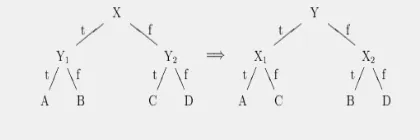
One of the two tree revision operators employed by ADT is to transpose a tree. When a different test should replace the current one at a decision node, each non-leaf subtree is first recursively revised so that the new test occurs at the root of each subtree. Then the tree is transposed at the decision node, as illustrated in Figure 2. One would rather not force a decision node into existence just for the sake of complying with the preconditions for the tree transposition operator. Instead, the tree transposition operator has been enhanced to handle the cases in which either subtree is a leaf.
An important observation is that the subtrees of the children of a node (A, B, C, and D in the figure 2) do not need to be examined or revised during tree transposition. Each subtree corresponds to a set of instances, and because that set has not changed during the transposition, the subtree does not need to be changed in any way. Similarly, the set of instances corresponding to the root of the tree being transposed does not change, and the test information maintained at that decision node does not change. For these reasons, only the information kept at the nodes of the two children (X1 and X2 in the figure) needs to be revised. This is done inexpensively,
without re-examining training instances, by simply combining the information kept in the each child's children nodes. For symbolic variables, one adds the frequency counts, and for numeric variables, one merges the two sorted value lists. Instances that may have been stored at each child node are simply removed and reincorporated at their parent node so that they find their way down to the proper node, typically a leaf.
Figure 2. Tree Transposition Operator
3.5 How to Ensure a Best Test Everywhere
We have seen how to bring a desired Boolean test to the root of a tree via transposition and by slewing. The general procedure for bringing a desired test, symbolic or numeric, to the root of a given subtree can now be stated. If the desired test is based on the current numeric variable, but the wrong cutpoint, then slew the cutpoint. Otherwise, if the desired test is based on the wrong variable, recursively bring the desired test to the root of each immediate nonleaf subtree and then transpose the tree. Finally, recursively ensure the best test for each of the two subtrees. As discussed above, one need not make the recursive call for a subtree that is not marked stale.
4. Experiments and results
4.1 Performance Study for updating model on various size of dataset
Table 1 shows the performance study of the update cost of the tree provided different size of datasets. The model is built on 10,000 instances dataset. The parameter values used to generate the dataset are as follows. The total number of attributes are 15 (including 5 numerical and 9 categorical). There are basically two class values for the class variable. The experiment result is shown in the Table 1. The experiments shows that update time would be affected by the number of instances applied for model update.
Table 1. Update time for the various size of dataset
No. of Records
No. of Records
added adaptively
C4.5 (in
seconds) Using ADT ( In Seconds)
10000
500 72.22 6.25 1000 76.45 10.73 1500 80.68 13.51 2000 86.17 16.95 2500 91.83 20.24
4.2 Scale up on number of attributes
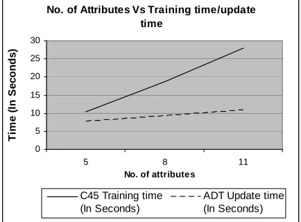
The experimental result is shown in Figure 2 which shows that with the increase in the number of attributes would increase in time for building tree from scratch. But once it has been built, then update time would be independent or nearly so, of number of attributes on which model built. The time increases because it requires more number of test to be carried out for testing at decision node. Once it is decided that which attribute is best at that node, then only instance to be incorporated in the dataset.
No. of Attributes Vs Training time/update time
0 5 10 15 20 25 30
5 8 11
No. of attributes
T
im
e
(
In
S
e
c
o
nd
s
)
C45 Training time (In Seconds)
ADT Update time (In Seconds)
Figure 3. scale up performance for various number of attributes
Table 2. scale up perforname for various number of attributes
no of attributes (10000 Records )
C4.5 training time ( In Seconds)
ADT Update time ( In Seconds)
5 10.33 7.61
8 18.61 9.23
11 28.04 10.78
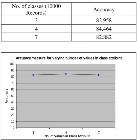
attribute. It is observed that accuracy can be achieved up to good level even though multiple classes to be handled by the method.
Table 3. discrete values in class attribute
No. of classes (10000
Records) Accuracy
3 82.958 4 84.464 7 82.882
Accuracy measure for varying number of values in class attribute
0 10 20 30 40 50 60 70 80 90 100
3 4 7
No. of Values in Class Attribute
A
ccu
rac
y
Figure 4. Performance study for accuracy for dataset with multiple classes
5. Conclusion
The ADT algorithm builds a decision tree incrementally, by restructuring the tree as necessary so that a best test attribute is at each decision node. Although the algorithm retains training instances within the tree structure, the instances are used only for restructuring purposes; they are not reprocessed. The notion of being able to revise a tree inexpensively makes searching the space of decision trees much more tractable because one can step from tree to tree more cheaply than one can generate each tree from scratch. The ADT algorithm can be viewed as an incremental variant of the ID3 tree building routine. The ADT algorithm takes very less time to make tree up to date then to induct tree from scratch on augmented dataset.
Several improvements for the ADT algorithm are possible. To improve the performance of the tree one should group values of a variable that have similar distribution of instances. This avoids excessive partitioning, generally reducing size and improving accuracy. Groping of variable can be done on symbolic and numerical type of variable.
6. References
[1] John Shafer, Rakesh Agrawal and Manish Mehta SPRINT: A Scalable Parallel Classifier for Data Mining. IBM Almaden Research Center,650 Harry Road,San Jose, CA 95120 [page no. 2-5]
[2] John Shafer, Rakesh Agrawal and Manish Mehta SLIQ : A fast scalable classifier IBM Almaden Research Center,650 Harry Road, San Jose, CA95120. [page no. 1-6]
[3] Lawrence O. Hall, Nitesh Chawla and Kevin W. Bowyer Decision tree learning on very large data set Department of Computer Science and Engineering, ENB 118, University of South Florida 4202 E. Fowler Ave.Tampa, Fl 33620 [page no. 2-4]
[4] Machine learning dataset http://www.ics.uci.edu/~mlearn/MLRepository.html
[5] Paul E. Utgoff. Decision Tree Induction Based on Efficient Tree Restructuring Department of Computer Science, University of Massachusetts, Amherst, MA 01003 Neil [email protected] Corvid Corporation, 779 West Street, Carlisle, MA 01741 [page no.1- 10]
[6] Saher Esmeir & Shaul Markovitch. Lookahead-based Algorithms for Anytime Induction of Decision Trees Department of Computer Science, Technion Israel Institute of Technology, Haifa 32000, Israel [page no. 2-6]