University of New Hampshire Scholars' Repository
Earth Sciences Scholarship
Earth Sciences
4-28-2016
Estimating Tropical Forest Structure Using a
Terrestrial Lidar
Michael W. Palace
University of New Hampshire - Main Campus, [email protected]
Franklin B. Sullivan
Earth System Research Center, Institute for the Study of Earth, Oceans, and Space, University of New Hampshire
Mark Ducey
Department of Natural Resources, University of New Hampshire, Durham, New Hampshire
Christina Herrick
Earth System Research Center, Institute for the Study of Earth, Oceans, and Space, University of New Hampshire
Follow this and additional works at:
https://scholars.unh.edu/earthsci_facpub
This Article is brought to you for free and open access by the Earth Sciences at University of New Hampshire Scholars' Repository. It has been accepted for inclusion in Earth Sciences Scholarship by an authorized administrator of University of New Hampshire Scholars' Repository. For more
information, please [email protected].
Recommended Citation
Palace, Michael W.; Sullivan, Franklin B.; Ducey, Mark; and Herrick, Christina, "Estimating Tropical Forest Structure Using a Terrestrial Lidar" (2016).PLOS ONE. 617.
Estimating Tropical Forest Structure Using a
Terrestrial Lidar
Michael Palace1,2*, Franklin B Sullivan1, Mark Ducey3, Christina Herrick1
1Earth System Research Center, Institute for the Study of Earth, Oceans, and Space, University of New
Hampshire, Durham, New Hampshire, United States of America,2Department of Earth Sciences, University
of New Hampshire, Durham, New Hampshire, United States of America,3Department of Natural
Resources, University of New Hampshire, Durham, New Hampshire, United States of America
Abstract
Forest structure comprises numerous quantifiable biometric components and characteris-tics, which include tree geometry and stand architecture. These structural components are important in the understanding of the past and future trajectories of these biomes. Tropical forests are often considered the most structurally complex and yet least understood of for-ested ecosystems. New technologies have provided novel avenues for quantifying biomet-ric properties of forested ecosystems, one of which is LIght Detection And Ranging (lidar). This sensor can be deployed on satellite, aircraft, unmanned aerial vehicles, and terrestrial platforms. In this study we examined the efficacy of a terrestrial lidar scanner (TLS) system in a tropical forest to estimate forest structure. Our study was conducted in January 2012 at La Selva, Costa Rica at twenty locations in a predominantly undisturbed forest. At these locations we collected field measured biometric attributes using a variable plot design. We also collected TLS data from the center of each plot. Using this data we developed relative vegetation profiles (RVPs) and calculated a series of parameters including entropy, Fast Fourier Transform (FFT), number of layers and plant area index to develop statistical rela-tionships with field data. We developed statistical models using a series of multiple linear regressions, all of which converged on significant relationships with the strongest relation-ship being for mean crown depth (r2= 0.88, p<0.001, RMSE = 1.04 m). Tree density was found to have the poorest significant relationship (r2= 0.50,p<0.01,RMSE= 153.28 n ha-1). We found a significant relationship between basal area and lidar metrics (r2= 0.75,
p<0.001,RMSE= 3.76 number ha-1). Parameters selected in our models varied, thus indi-cating the potential relevance of multiple features in canopy profiles and geometry that are related to field-measured structure. Models for biomass estimation included structural can-opy variables in addition to height metrics. Our work indicates that vegetation profiles from TLS data can provide useful information on forest structure.
a11111
OPEN ACCESS
Citation:Palace M, Sullivan FB, Ducey M, Herrick C (2016) Estimating Tropical Forest Structure Using a Terrestrial Lidar. PLoS ONE 11(4): e0154115. doi:10.1371/journal.pone.0154115
Editor:RunGuo Zang, Chinese Academy of Forestry, CHINA
Received:January 7, 2016
Accepted:April 8, 2016
Published:April 28, 2016
Copyright:© 2016 Palace et al. This is an open access article distributed under the terms of the
Creative Commons Attribution License, which permits
unrestricted use, distribution, and reproduction in any medium, provided the original author and source are credited.
Data Availability Statement:Data are all contained within the paper, additional raw data (not part of the minimal underlying dataset) is available by contacting the author due to the immense storage volume.
Introduction
Forest structure is a reflection of the principles of forest growth and disturbance, influenced by the spatial and temporal variability of resource availability, disturbance rates, and management [1–4]. The three dimensional architecture of a forest is a direct indication of ecosystem func-tion, carbon and nutrient cycling, disturbance regimes, and the coupling between forests and regional and global climate [5]. Tropical forests have additional complexity in regard to species diversity and are thought to be among the most structurally complex of all forested ecosystems [6]. Tropical forest structure characterization is important in understanding ecological and earth system processes, knowledge of which proves vital in efforts to mitigate climate change through the reduction of greenhouse gases emissions. The ability to quantify forest structure beyond standing biomass is critical to efforts such as Reducing Emissions from Deforestation and Forest Degradation (REDD+), which depends on characterization of forest structure to provide insight into the previous carbon dynamics and the potential future storage capabilities of a forest [7–10]. Ground-based measurements allow for accurate mapping of vegetation structure, but only on very limited spatial and temporal scales, and with high costs and unknown biases [11].
The spatial variability of forest structure at the landscape scale is difficult to capture without remote sensing methods because proper evaluation of variability across the landscape would require extensive field campaigns, which can be cost prohibitive. To extract information related to changes in forest structure, measurements on the ground must be associated with those inferred from airborne and space-based remote sensing data [12–13]. Research and field sites that have both extensive field-based biometric data as well as remote sensing data are vital in estimating forest biometric properties. New technologies, such as LIght Detection And Ranging (lidar), offer the possibility of reducing inventory costs and increasing accuracy [14]. Lidar remote sensing has been used to estimate the horizontal and vertical heterogeneity in forest structure [15–19] and can be deployed from space, aircraft, and on the ground. Previous stud-ies have demonstrated that airborne lidar-derived canopy vegetation profiles compare well with ground-based profiles [20–21]. Canopy vegetation profile metrics have been shown to be useful in predicting biomass and other structural forest properties [8,17,22–32]. A majority of effort has been to use discrete airborne lidar, yet ground-based lidar deployment may provide additional insight and is currently being deployed in many forested settings [33–37].
Ground-based imaging lidar systems often gather a detailed, three-dimensional digital model of forest stands and individual trees from an understory perspective [38]. These systems can be deployed quickly in multiple locations and gather information often faster than those collected by field crews and measure unique attributes often complementing field-based sur-veys [39–40]. In particular, ground-based lidar may be useful for reducing uncertainty associ-ated with the generalized allometric equations used to convert standard tree measurements to biomass or carbon; error in allometrics is a key source of uncertainty in large-scale inventories, and does not decline with increased sampling intensity or number of plots [11,41]. Terrestrial laser scanners were originally designed for precision surveying applications; applications to for-est ecosystem measurement are just emerging [42]. Algorithms to estimate aboveground forest biomass, its components (foliage, stemwood, and branchwood), and their three-dimensional distribution are in their infancy but show great promise [43–45].
In this study, we focused on the utility of canopy profiles derived from TLS data for develop-ing relationships to field data, similar to approaches that use airborne lidar scanners. Method-ology for the calculation of RVPs is described in detail. We evaluated statistical relationships between TLS canopy profiles and associated metrics with field-measured biometric properties for twenty plots within La Selva Biological Station, Costa Rica. We used multivariate linear
regression with stepwise variable selection to develop models of forest biometric properties from a suite of canopy profile metrics.
Methods
Study site and data sets
La Selva. We conducted our research at the La Selva Biological Station (10° 26’N, 83° 59’ W), operated by the Organization for Tropical Studies and located in the Atlantic lowlands of Costa Rica [46]. We determined the location of twenty plots that were randomly selected to measure field-based biometric properties and collect ground-based terrestrial lidar scans. We selected our plot locations using a set ofa prioriconstraints based on GIS data layers (trails existing studies, water bodies, vegetation type) provided by the La Selva (http://www.ots.ac.cr). Criteria for our plot selection included ease of access, with sites being chosen that were within 100 m and greater than 30 m of established trails. Sites were selected within 50 m from rivers and water bodies to minimize the influence of local topography and additional effort required when measuring forested plots in wetlands. There are also a great deal of permanent plots at La Selva, so to avoid disturbing ongoing long term research, we selected plots that they were at least 25 m away from established study areas. Locations of random plots did not require spe-cific permission by the reserve, nor did our field research involve any endangered or protected species. Field plots were located using a Garmin 76CSx GPS.
Field biometric measurements. For each of the twenty plots we measured stand and tree attributes using a variable plot design. Trees were counted using a Spiegel-relaskop using a basal area factor (BAF) of 4 m2ha-1at the plot center and at four satellite plots spaced 30 m from the plot center on each of the cardinal directions [47]. We chose this sampling method because the variable plot radius design allows for a stratified sampling of trees that are more likely to contribute to the canopy above a specific point. For sampled trees, we measured diam-eter at breast height (dbh) using a diamdiam-eter tape, total height, and height to the base of the live crown for all trees using a Vertex hypsometer (Haglof Inc.). Buttressed trees that proved diffi-cult in the measurement of dbh at the usual height (1.37 m) were measured directly above the buttresses optically using the Spiegel-relaskop at a known distance from the tree [48]. This method has been found to be more efficient and just as accurate in estimating DBH [48].
We conducted our field measurements in January 2012. We sampled plots located in old growth, abandoned pasture (approximately 70 years), and logged and secondary forest types. Basal area (area of the cross section of trees at breast height per total area) was measured on all 20 plots and four additional plots for each of the twenty primary plots for a total of 80 satellite plots. These 80 satellite plots also used the same variable size plot design. Our stratified sam-pling design yielded trees of all dbh sizes classes, thus providing a good indication of canopy contribution for comparison with lidar data. The quadratic stand diameter (QSD) was also cal-culated from plot-level summary data. This is determined from the equation from [49]:
QSD¼
ffiffiffiffiffiffiffiffiffiffiffiffiffiffiffiffiffiffiffiffiffiffiffiffiffiffiffiffi
BA
N
4
p s
which is a plot-level basal area weighted mean height. Plot locations and measured biometric properties were presented in [19].
Terrestrial Laser Scanner (TLS). We used a FARO Focus 3D for our TLS scans, with a narrow beam width (~5mm at 50m range). The TLS returns approximately 40 million points per plot. Scans were conducted in the center of our field measured plots. Examples of terrestrial lidar scans are presented inFig 1. This instrument weighs 5.2 kg, and is deployed on a light-weight carbon fiber tripod. It is self-contained and transported in a weatherproof field case,
Fig 1. Terrestrial based lidar (TLS) scans of tropical forest on a hillslope at La Selva Biological Reserve, Costa Rica.Top-Color indicates distance from scanner, while saturation indicates laser reflectivity. Distortion of canopy elements near the top of the image is due to cylindrical reprojection of a
hemispherical scan. Note that the image here is a 100x downsampling of the original scan, which includes over 40 million (x,y,z) coordinates. Bottom-Higher
resolution TLS image focusing on the understory, white indicates closer objects, black indicates more distant returns.
and capable of operating on a single internal rechargeable battery to conduct multiple scans over a full field day. Data is collected on a Secure Digital card (SD), allowing for an entire day of field data to be stored.
Scans were recorded in the center of our field-plots. When single-scan TLS is employed to recover the size, characteristics, and position of individual tree stems, occlusion by other vege-tation can present significant challenges, leading to non-detection bias ([53–54] for corrective techniques). However, in this study, the focus is on the recovery of bulk canopy attributes, and we employ a statistical approach based on a modified MacArthur and Horn estimator [55], that specifically accounts for occlusion, described in section 2.2.1 Relative vegetation profiles.
Processing
Relative vegetation profiles. To construct vertical profiles of plant surface area from TLS scans, we adopted a quasi-likelihood approach, following [56]. The approach builds on the connection between the MacArthur-Horn estimator [55] and the family of statistical tech-niques known as survival analysis [57].
Consider a volume element defined in 3-dimensional space, penetrated bynTLS probes. Letβidenote the angle of elevation of the ithprobe above the horizontal plane. We model the
distribution of plant surfaces using a set ofmdiscrete classes; denote the inclination of thejth class relative to the horizontal asαj, and its density (m2/m3of projected surface area) asρj. We
assume either that the distribution of surface angles is radially symmetrical, or that the distri-bution of probes is; the latter assumption is appropriate for tripod-mounted TLS with volume elements centered over the tripod position. Then the apparent density of surfaces, normal to a probe with angleβi, is
Fbi¼X
j
gaj;birj
where (following [58])
gaj;bi ¼ cosajsinbi ajbi
gaj;bi¼
2
psinajcosbisiny0þ 1 y0 90
cosajsinbi ajbi
and
y0¼cos1ðcotajtanbiÞ
Now, let libe the length of the ithprobe within the volume element (originating at the TLS
unit, or on a boundary surface of the volume element; and terminating either on contact with a surface, or by exiting the volume element). Let di= 0 indicate that the ithprobe contacted a
sur-face, and di= 1 indicate that it exited the volume element without contact. Then, treating then
probes as independent observations, following the general model of [56] the log-likelihood of the observed data can be written as
lnL¼X
n
i¼1
liFbiþ ðldiÞlnðFbiÞ
equation, subject to the constraint thatρj0 for all classes, using m = 9 angle classes (centered
on 5, 15, 25,. . ., 85 degrees from the horizontal). The horizontal projection of the surfaces within each angle class was then summed to yield the vertical distribution of horizontally-pro-jected plant surfaces.
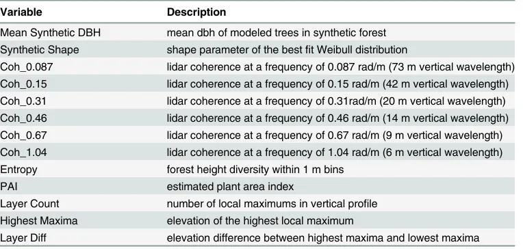
Parameters from RVPs. From RVPs, we calculated a series of metrics for developing sta-tistical relationships between lidar data and field-based vegetation structural components (Table 1), which we used previously in a study comparing canopy profiles developed from air-borne lidar [19]. The metrics we used for our analysis include a profile layer count, peak max-ima (i.e. height above ground of the largest maximum), highest maxmax-ima (i.e. height above ground of the highest maximum), profile median height, and a ratio of median height to maxi-mum height of each profile. In addition, we calculated entropy [19,59], and lidar coherence of Fourier transforms, using Fast Fourier Transforms (FFT) at frequencies of 0.087 rad m-1, 0.15 rad m-1, 0.31 rad m-1, 0.46 rad m-1, 0.67 rad m-1, and 1.04 rad m-1[60], which have been shown to be correlated with biomass when using airborne lidar data. These frequencies corre-spond to so-called vertical wavelengths of 73, 42, 20, 14, 9, and 6m, respectively. FFT parame-ters do not include phase.
Theoretical stands, synthetic forests and vegetation profiles. Tree height, crown geome-try, light dynamics, and canopy foliage have been linked to tree trunk diameters through allo-metric equations [59,61–65]. Through the comparison of tree trunk diameter groups, specific insight may be gleaned in regard to growth and disturbance dynamics [1,66]. Ratios compar-ing successive diameter classes tend to be consistent for a forest that is considered to be at or near a steady state [67–68]. These ratios are often termed q-ratios because of the "quotient of diminution" or rate of change between diameter classes [68–69]. A constant q-ratio is also expressed as an exponential diameter distribution [11,67,68,70]. It was determined that q var-ied within stands [69], despite much literature focusing on a constant q in mixed age states or exponential distribution. The Weibull distribution includes the constant-q as a special case when the shape parameter is set to one [71].
Previously, we developed synthetic forest algorithm that uses geometric series to generate forest stands [19,72]. Our model uses allometric equations that relate crown size to dbh [12,
73]. Using a random tree trunk size pulled from a Weibull distribution, we place the tree on the landscape (horizontal location). For each tree placed on the landscape, we generate an ellipsoid in three dimensional space based on these parameters (dbh and crown geometry) to develop a
Table 1. Description of lidar-derived vertical profile metrics.
Variable Description
Mean Synthetic DBH mean dbh of modeled trees in synthetic forest
Synthetic Shape shape parameter of the bestfit Weibull distribution
Coh_0.087 lidar coherence at a frequency of 0.087 rad/m (73 m vertical wavelength)
Coh_0.15 lidar coherence at a frequency of 0.15 rad/m (42 m vertical wavelength)
Coh_0.31 lidar coherence at a frequency of 0.31rad/m (20 m vertical wavelength)
Coh_0.46 lidar coherence at a frequency of 0.46 rad/m (14 m vertical wavelength)
Coh_0.67 lidar coherence at a frequency of 0.67 rad/m (9 m vertical wavelength)
Coh_1.04 lidar coherence at a frequency of 1.04 rad/m (6 m vertical wavelength)
Entropy forest height diversity within 1 m bins
PAI estimated plant area index
Layer Count number of local maximums in vertical profile
Highest Maxima elevation of the highest local maximum
Layer Diff elevation difference between highest maxima and lowest maxima
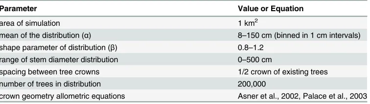
forest canopy. If there is too much overlap, i.e. crown shying or light competition, we deter-mine another random horizontal location for the tree and repeat the check on crown overlap. Crown overlap of less than half of the horizontal radius of any crown was used in our model and results in field-based measurements of gap values [72,74]. Parameters used in our syn-thetic forest model are found inTable 2. Our method for developing a vegetation profile based on theoretical stand information is still novel and is explored in [19,21], and utilized for stand metrics in [72]. We note that other scientific disciplines have used theoretical models of physi-cally based systems to interpret observed phenomena, such as exoplanet ring systems [75–76].
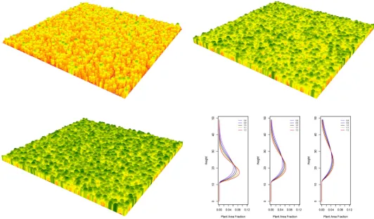
Three-dimensional synthetic forest canopies were aggregated to represent vertical profiles derived from Weibull attributes (Fig 2). We generated thousands of synthetic forests and their resulting vertical profiles. Once normalized the relative vegetation profiles were compared with the lidar RVPs. A goodness-of-fit was used to determine which synthetic vegetation profiles best matched a lidar RVP. The Weibull distribution parameters represented by the best fit syn-thetic forest profile were then used in the development of multiple linear regressions along with other parameters (entropy, PAI, FFT, etc.). We stress that these parameters were represen-tative of theoretical forests and provided an additional means to characterize terrestrial lidar information. Currently, our model is able to ingest spatial point data from field plots and develop a three dimensional canopy. In our efforts to develop theoretical forests stands, we rely on randomly pulling a tree diameter from a distribution and then randomly placing it across the landscape, using crown overlap as the spacing mechanism. There are other approaches to modeling efficient tree and crown spacing, such as spatial point processes, but we have opted for a simpler approach for this model.
Statistics and Computational Coding
Our estimates of theoretical forests and the associated synthesized vegetation profile utilized code developed in Python 2.7 (Python Software Foundation, Python version 2.7,www.python. org). Multiple regression models using forward stepwise regression with Bayesian information criteria (BIC) for variable inclusion in the model were developed using field-measured forest structure and terrestrial lidar metrics [19,77], including estimates of forest gappiness, canopy layers, and comparisons with our theoretical forest vegetation profile. We also used the FFT analysis for in our model development. Numerous other variables were calculated for this study, such as percentile scores for the RVP, however we specifically chose variables to explore that could be interpreted as biophysical attributes of the vegetation profile. Python 2.7 was used to derive lidar metrics and for a least-squares analysis to compare theoretical profiles with TLS derived profiles. We used JMP10 Pro (www.jmp.com) for regression model development. Multiple regression analysis is specifically designed to accommodate correlated variables; there is no requirement that the variables be orthogonal. We used Bayesian information criterion in
Table 2. Synthetic forest parameterization.
Parameter Value or Equation
area of simulation 1 km2
mean of the distribution (α) 8–150 cm (binned in 1 cm intervals)
shape parameter of distribution (β) 0.8–1.2
range of stem diameter distribution 0–500 cm
spacing between tree crowns 1/2 crown of existing trees
number of trees in distribution 200,000
crown geometry allometric equations Asner et al., 2002, Palace et al., 2003
our stepwise variable selection. This is a method to allow for variable inclusion, but not at the expense of overfitting, by including a penalty term for the number of parameters in the model. The use of stepwise should only select variables that add to building a more significant model and parameters that are highly correlated may only have one of the variables included due to the second correlated variable not contributing to the model’s performance.
Results
Field-based Measurements
Field-measured forest structural data for the twenty plots were presented in [19]. We note that the forests examined in [19] and in this paper are high biomass and tall statured ranging in bio-mass from 190.3 to 362.4 Mg ha-1and average tree height from 10.12 to 39.20 m.
Lidar Metrics
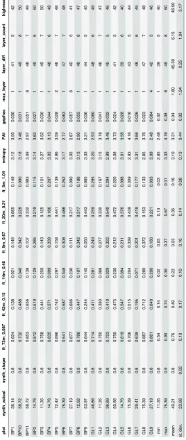
Metrics derived from the RVPs generated from the terrestrial lidar point cloud data are pre-sented inTable 3. Metrics are discussed here in the range of estimates, as well as the mean and standard deviation. Metrics derived from synthetic profiles developed from our theoretical for-est model for mean dbh ranged from 11.35 to 75.39 cm and the shape of the profile showed lit-tle different with only plot BP8, not being a 0.8, but rather 0.9. We stress that these values are
Fig 2. Examples of synthetic forests, with areas representing 1 km2.Colors indicate height at top of the canopy. Shown here are forests and profiles with mean diameters of 15 cm (left), 30 cm (middle) and 55 cm (right), with the shape parameter of the Weibull distribution varied from 0.8 to 1.2 in increments of 0.1.
not specifically comparable to field measured values, but provide a method to cull more infor-mation from the RVP generated from the ground-based terrestrial lidar data.
Transformed RVPs were used for lidar metrics except the FFT analysis which used untrans-formed data. This was done to follow the methodology used in [60] and then in [19]. Fourier transforms for a coherence of 0.087 rad m-1coherence (vertical wavelength of 73 m) ranged from 0.54 to 0.90. At a frequency of 0.15 rad m-1coherence (vertical wavelength of 42 m) ran-ged from 0.14 to 0.74. Values ranran-ged from 0.02 to 0.39 for a frequency of 0.46 rad m-1 coher-ence (vertical wavelength of 14 m). Fourier amplitudes for a cohercoher-ence of 0.67 rad m-1 coherence (vertical wavelength of 9 m) ranged from 0.05 to 0.37. Values ranged from 0.13 to 0.67 for a frequency of 0.31 rad m-1coherence (vertical wavelength of 20 m). Amplitudes from the Fourier transforms for a coherence of 1.04 rad m-1(vertical wavelength of 6 m) ranged from 0.03 to 0.31.
Entropy estimates from the lidar derived and transformed RVP ranged from 2.85 to 3.33, with the higher value indicating both a canopy that has more depth and that is more complex in layering. PAI ranged from 2.48 to 4.16 with the upper bound indicating more plant material over a given plot in the trees and canopy, but with no differentiation between leaves, stems, or branches. Gap fraction ranged from 0.02 to 0.08 with the higher value indicating a greater change of canopy penetration of light and the possibility of either disturbances or multi-layered nature of the forest. The number of estimated canopy layers ranged from 1 to 8, with the higher value representing a more complex canopy with a number of different tree crowns at differing heights. The height difference in the layers in meters ranged from 39 m to 49 m, with this met-ric being an indication of canopy depth. If only one layer was estimated this was the depth of that layer, and if multiple layers were found, this was the depth of all layers combined. Finally, we found that the height of the highest layer ranged from 40 to 50 m, indicating a rather tall statured forest.
Multiple Linear Regressions
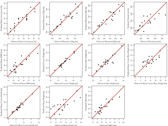
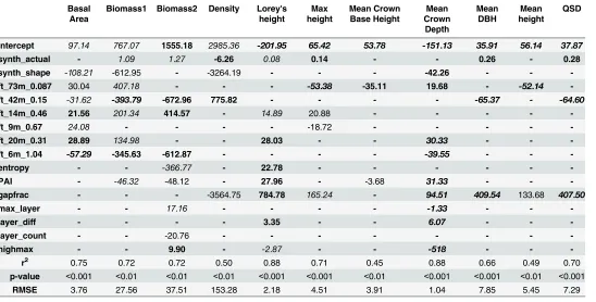
We developed a multiple linear regression using forward stepwise variable selection with BIC criteria for variable inclusion (Fig 3). A regression was developed for each of the field-measured or derived forest structural properties (Table 2). Model results are presented inTable 4and present estimators of lidar metrics, adjusted r-squared values, significance of the model, and root mean squared error (RMSE). Moderate to strong relationships between field-measured traits and a suite of metrics derived from the vegetation profiles we developed using lidar data (lidar metrics) were found with all models converging on a statistically significant model to estimate specific forest structural attributes.
significant relationship was found for mean crown depth (r2= 0.88,p<0.001,RMSE= 1.04 m). Lidar metrics for quadratic stand diameter and mean dbh were found to develop significant relationships (r2= 0.70,p<0.001,RMSE= 7.29 cm;r2= 0.49,p<0.01,RMSE= 5.45 m2).
Discussion
In this study, we collapsed the three-dimensional point cloud from a TLS into a two-dimen-sional canopy profile. We were able to predict many forest structural attributes, thus confirm-ing the usefulness of a TLS for forest inventory (Fig 3). Our work indicates that a terrestrial lidar sensor can provide useful information on forest structure [19] and comparison can be readily made between different sensors, in this case TLS, and field-measurements as shown in [21]. Still, the reduction to a two-dimensional data source loses a great deal of spatial informa-tion that might be useful for discerning addiinforma-tional forest structure, particularly in the under-story. TLS data can be reanalyzed with new algorithms and statistical analysis and can prove useful to examine new avenues of scientific questioning. This provides a unique opportunity to
Fig 3. Observed verses predicted forest biometric properties based on multiple linear regression models using stepwise variable selection.
provide a snapshot of a forest inventory plot, allowing for reexamination, analysis, and check on recorded information.
The three dimensional canopy can be integrated and expressed in two dimensions using a vegetation profile, which is a model of the distribution of vegetation as a function of height. We found that metrics derived from these profiles provide insight into biometric properties, rang-ing from biomass to density of trees. We were able to develop significant relationships between these profile metrics and forest structural attributes. There were numerous variables that could be used for the development of multiple regression models, but for this analysis we chose to examine information derived from our theoretical stand model and lidar profile parameters not typically used in forest biometric studies.
The variable radius plot design with a stratified sampling approach that we used in this study proved advantageous both for developing relationships between TLS data and biometric properties, and for conducting field measurements. We stress that the variable radius plot design provides a rapid and rigorous assessment of the forest structure. This is because it does not over sample smaller trees, allows for the inclusion of trees that contribute to canopy struc-ture, and provides estimates of basal area and its related properties, such as Lorey’s height, which are often used in remote sensing efforts. This approach made field work efficient and effective, evidenced by rapid field data collection (approx. 1 hour per plot). The TLS took
Table 4. Forest biometric properties and estimators from lidar metrics.
Basal Area
Biomass1 Biomass2 Density Lorey's height
Max height
Mean Crown Base Height
Mean Crown
Depth
Mean DBH
Mean height
QSD
Intercept 97.14 767.07 1555.18 2985.36 -201.95 65.42 53.78 -151.13 35.91 56.14 37.87 synth_actual - 1.09 1.27 -6.26 0.08 0.14 - - 0.26 - 0.28 synth_shape -108.21 -612.95 - -3264.19 - - - -42.26 - - -ft_73m_0.087 30.04 407.18 - - - -53.38 -35.11 19.68 - -52.14 -ft_42m_0.15 -31.62 -393.79 -672.96 775.82 - - - - -65.37 - -64.60 ft_14m_0.46 21.56 201.34 414.57 - 14.89 20.88 - - - -
-ft_9m_0.67 24.08 - - - - -18.72 - - - -
-ft_20m_0.31 28.89 134.98 - - 28.03 - - 30.33 - - -ft_6m_1.04 -57.29 -345.63 -612.87 - - - - -39.55 - -
-entropy - - -366.77 - 22.78 - - -
-PAI - -46.32 -48.12 - 27.96 - -3.68 31.33 - -
-gapfrac - - - -3564.75 784.78 165.24 - 94.51 409.54 133.68 407.50
max_layer - - 17.16 - - - - -1.33 - -
-layer_diff - - - - 3.35 - - 6.07 - -
-layer_count - - -20.76 - - - - - - -
-highmax - - 9.90 - -2.87 - - -518 - -
-r2 0.75 0.72 0.72 0.50 0.88 0.71 0.45 0.88 0.66 0.49 0.70
p-value <0.001 <0.01 <0.01 <0.01 <0.001 <0.001 <0.01 <0.001 <0.001 <0.01 <0.001
RMSE 3.76 27.56 37.51 153.28 2.18 4.51 3.91 1.04 7.85 5.45 7.29
p<0.001
p<0.01
p<0.05
p>0.05
r2values presented are adjusted r2values because of inclusion of additional variables.
fifteen minutes to collect, with new instruments providing high resolution and faster collection times. We suggest that the TLS is a highly useful and robust technique for quantifying forest structure, specifically in a tropical forest, where field effort is often high. We also note the use-fulness of a TLS in conjunction with field plot measurements.
Field-based measurements were presented in [19] and are on par with those found from other studies at La Selva [60,78–80]. In addition, our measured canopy height was consistent with that found in [28]. We found that many of the geometric canopy properties have not been measured in the field at La Selva, but were comparable to results from tropical forests in Ama-zonia and the pan-tropical regions [12,63,64,73]. We stress that measurements other than just height are important in the understanding of forest dynamics and should be included in inventory efforts [19,78,80]. We note that the forests examined in [19] and in this paper are higher biomass tropical forests with less range in biomass than some other studies. The limited range in both height and biomass complicated our efforts, but nevertheless we were able to develop significant statistical models. We suggest that our approach could be used to improve and refine biomass estimation for REDD+ efforts.
Theoretical forest stands and synthetic vegetation profile
The synthetic vegetation profile allowed for theoretical stand distributions to be compared with vegetation profiles developed from discrete return lidar data. This was specifically used to retrieve additional information about stand size class distributions from the lidar profile. In essence, the synthetic forest algorithm develops numerous vegetation profiles based on two parameters from a theoretical model. The two parameters (shape and mean of a forest dbh dis-tribution) drive the modeled stand conditions, and therefore the thickness of the vegetation profile and the overall height. This is because dbh and height of vegetation are related, but other forest structural properties are more complex than just maximum height. The distribu-tion of trees in various dbh classes represented by the Weibull distribudistribu-tion used in our syn-thetic forest model represent the canopy structure and vegetation profile of hyposyn-thetical forests.
old-growth forests. The alteration of the proportion of tree stand size classes may indicate a distur-bance [66]. Other regressions that utilized the shape parameter for the synthetic profile are the basal area, biomass2, and mean crown depth. The results of this study with regard to theoretical forest stand profiles warrant further investigation of the use of this approach for interpretation of forest disturbance and past human activity. We suggest the use of this model comparison approach to aid in the possible interpretation of forest disturbance and past human activity.
Fast Fourier Transforms and other Canopy Profile Metrics
Magnitudes of coherence of Fast Fourier Transforms of canopy height profiles provide insight into the canopy structure [19,81]. The frequencies used in this study correspond to wave-lengths that are structurally significant in La Selva and have been shown to be particularly use-ful for estimating biomass using airborne lidar and radar [60]. For example, mean canopy depth at La Selva averages around 7 m and mean canopy height averages around 22 m [19]. The coherence of the frequencies corresponding to these wavelengths were significant in our analysis, as has been shown in previous studies [19,60,81]. This can provide some indication of the structurally significant features that are present in the canopy height profile. In terms of biomass estimation, characterizing the structure of the canopy by coherence of frequencies cor-responding to features like depth and canopy height can serve as an analog for the amount of canopy material present. In previous studies, lidar coherence was calculated using canopy pro-files derived from airborne lidar data. It is notable that in this study we achieved similar results using terrestrial-based lidar systems, which implies that structural features present in canopy profiles can be observed using above or below canopy sensors. Our analyses included frequen-cies corresponding to vertical wavelengths of 73, 42, 20, 14, 9, and 6m, respectively. These echo strong forest height signals of approximately mean crown depth and mean tree height in our study.
Merits of Multiple Linear Regressions
We found that the TLS provides good estimates of canopy properties when modeled using multiple linear regression of metrics derived from canopy profiles. The best performing model developed in this study was for mean crown depth (r2= 0.88,p<0.001,RMSE= 1.04 m). This model also includes the most variables in the construction of all of our multiple regressions. Although regression models containing many parameters are thought to be problematic due to overfitting, we stress that with BIC variable selection, this was not the case. BIC variable selec-tion favors the exclusion of unnecessary variables from models. Model performance provided insight into the complexity of forest structure as measured using terrestrial lidar scans, and also hinted at how canopies are organized in forested ecosystems.
The regression model developed to estimate stand density (number per hectare) only include two lidar metrics, shape of the synthetic profile diameter distribution (synth_shape) and FFT coherence (0.087). The model also had a significant, but rather low r2value compared to other models (r2= 0.50,p<0.01,RMSE= 153.28 n ha-1). The coherence at a frequency of 0.087 rad/m, corresponding to a vertical wavelength of 73 meters, was positively related to stand density. A taller forest in a primary forest often has more stems because the complex gal-lery forest allows for smaller trees to begin growing underneath in a multi-aged and tiered for-est and canopy when compared to an even-aged forfor-est of similar average height.
variables indicates the importance of looking at FFTs in the estimation of biomass in tropical forests using TLS. These variables represent the relative layering and complexity of the forest canopy, with a mixed age stand exhibiting a more complex canopy and containing higher bio-mass due to the optimal space packing of canopy architecture. Improvements in the disordered packaging using ellipsoids have been explored and may be comparable to the crown geometric space filling of tree canopies [82–83]. Supporting this is also the inclusion of entropy of the RVP for the biomass1 model, which is indicative of the complexity of canopy vegetation distri-bution. PAI and maximum layer height were included for both biomass estimates. Biomass1 also included a negative relation with layer count and a positive relation with maximum height. The estimated dbh from the synthetically derived RVP was used in both regressions and bio-mass2 also included a negative relation with the shape of the synthetic RVP.
Biomass is often the structural characteristic of forests that is of highest interest due to REDD+ efforts, but this focus neglects additional forest structural information that can be used to infer the past and future trajectory of forest stands. The estimation of such characteristics, such as basal area, areal density, crown geometry, and size class distribution, are within reach using either airborne or terrestrial lidar systems. We focus on biomass because it is easier to estimate across a broad range of values, ranging from lower secondary estimates to higher full stature forests. However, much of the focus of biomass estimation efforts has been in higher biomass tropical forests, where remote sensing efforts can fall short due to instrument limita-tions (e.g. saturation) or issues with linking plot level estimates with moderate scale remote sensing image data. The estimation of biomass even within and across high biomass forests is possible with lidar data, but requires quality field-data for statistical model development. Fur-ther, lidar data are particularly amenable to biomass estimation in high biomass forests because of the wealth of information about forest stands that can be retrieved from lidar-derived vege-tation profiles, which we presented in this paper.
Conclusions
Acknowledgments
This research was supported by NASA New Investigators in Earth Science (NNX10AQ82G), NASA Terrestrial Ecology (NNX08AL29G), NASA IDS (NNX14AD31G) and USAID (12DG11132762416). We thank La Selva Research Station for accommodations and use of their GIS data. We also thank Julia Shimbo and Jonas Mota e Silva for aid in field work. We also thank three anonymous reviewers for their effort and time that made this paper much improved.
Author Contributions
Conceived and designed the experiments: MP MD. Performed the experiments: MP MD CH. Analyzed the data: MP FBS MD. Contributed reagents/materials/analysis tools: MP MD FBS CH. Wrote the paper: MP FBS MD.
References
1. Oliver CD, Larson BC. Forest Stand Dynamics, Updated edition. New York: Wiley; 1996.
2. Franklin JF, Spies TA, Van Pelt R, Carey A, Thornburgh D, Berg DR, et al. Disturbances and the
struc-tural development of nastruc-tural forest ecosystems with some implications for silviculture. For Ecol
Man-age. 2002; 155: 399–423.
3. Palace M., Keller M, Hurtt H, Frolking S. A review of above ground necromass in tropical forests. In:
Sudarshana P, Soneji Nageswara-Rao, editors. Tropical Forests. InTech; 2012.
4. Espírito-Santo FDB, Gloor M, Keller M, Malhi Y, Saatchi S, Nelson B, et al. Size and Frequency of
Natu-ral Forest Disturbances in Amazonia. Nat Commun 2014; doi:10.1038/ncomms4434
5. Tang H, Dubayah R, Brolly M, Ganguly S, Zhang G. Large-scale retrieval of leaf area index and vertical
foliage profile from the spaceborne waveform lidar (GLAS/ICESat). Remote Sens Environ 2014; 154:
8–18.
6. Whitmore TC. On pattern and process in forests. In: Newman EI, editor. The Plant Community as a
Working Mechanism. Blackwell Scientific Publications, Oxford; 1982. pp. 45–59.
7. Asner GP. Painting the world REDD: addressing scientific barriers to monitoring emissions from tropical
forests. Environ Res Lett 2011; 9(2): doi:10.1088/1748-9326/6/2/021002
8. Asner GP, Mascaro J, Anderson C, Knapp DE, Martin RE, Kennedy-Bowdoin T, et al. High-fidelity
national carbon mapping for resource management and REDD+. Carbon Balance and Management
2013; doi:10.1186/1750-0680-8-7
9. Berenguer E, Ferreira J, Gardner TA, Aragão LEOC, De Camargo PB, Cerri CE, et al. A large-scale
field assessment of carbon stocks in human-modified tropical forests. Glob Chang Biol 2014; doi:10.
1111/gcb.12627
10. Bustamante MC, Roitman I, Aide T, Alencar A, Anderson L, Aragão LE, et al. Towards an integrated
monitoring framework to assess the effects of tropical forest degradation and recovery on carbon
stocks and biodiversity. Glob Chang Biol 2015; doi:10.1111/gcb.13087
11. Keller M, Palace M, Hurtt G. Biomass estimation in the Tapajos National Forest, Brazil: Examination of
sampling and allometric uncertainities. For Ecol Manage 2001; 154(3): 371–382.
12. Palace M, Keller M, Asner GP, Hagen S, Braswell B. Amazon forest structure from IKONOS satellite
data and the automated characterization of forest canopy properties. Biotropica 2008; 40(20): 141–
150.
13. Frolking S, Palace M, Clark DB, Chambers JQ, Shugart HH, Hurtt GC. Forest disturbance and recovery
—a general review in the context of space-borne remote sensing of impacts on aboveground biomass
and canopy structure. J Geophys Res 2009; 114: G00E02, doi:10.1029/2008JG000911
14. Chambers JQ, Asner GP, Morton DC, Anderson LO, Saatchi SS, Espírito-Santo FDB, et al. Regional
ecosystem structure and function: Ecological insights from remote sensing of tropical forests. Trends
Ecol Evol 2007; 22(8): 414–423. PMID:17493704
15. Vierling LA, Rowell E, Chen X, Dykstra D, Vierling K. Relationships among airborne scanning lidar,
high resolution multispectral imagery, and ground-based inventory data in a ponderosa pine forest.
Geoscience and Remote Sensing Symposium, 2002. IGARSS‘02. 2002 IEEE International (vol. 5)
Toronto, Canada.
16. Jensen JR, Humes KS, Vierling LA, Hudak AT. Discrete return lidar-based prediction of leaf area index
17. Tang H, Dubayah R, Swatantran A, Hofton M, Sheldon S, Clark DB, et al. Retrieval of vertical LAI pro-files over tropical rain forests using waveform lidar at La Selva, Costa Rica. Remote Sens Environ
2012; 124: 242–250.
18. Whitehurst AS, Swatantran A, Blair JB, Hofton MA, Dubayah R. Characterization of canopy layering in
forested ecosystems using full waveform lidar. Remote Sens 2013; 5: 2014–2036.
19. Palace M, Sullivan FB, Ducey MJ, Czarnecki C, Zanin Shimbo J, Mota e Silva J. Estimating forest
struc-ture in a tropical forest using field measurements, a synthetic model and discrete return lidar data.
Remote Sens Environ 2015; 161: 1–11. doi:10.1016/j.rse.2015.01.020
20. Harding DJ, Lefsky MA, Parker GG, Blair JB. Laser altimeter canopy height profiles: Methods and
vali-dation for closed-canopy, broadleaf forests. Remote Sens Environ 2001; 76(3): 283–297.
21. Sullivan FB, Palace M, Ducey MJ. Multivariate statistical analysis of asynchronous lidar data and
vege-tation models in a neotropical forest. Remote Sens Environ 2014;
22. Lefsky MA, Cohen WB, Acker SA, Parker GG, Spies TA, Harding D. Lidar remote sensing of the canopy
structure and biophysical properties of Douglas-fir western hemlock forests. Remote Sens Environ
1999; 70(3): 339–361.
23. Means JE, Acker SA, Harding DJ, Blair JB, Lefsky MA, Cohen WB, et al. Use of large-footprint scanning
airborne lidar to estimate forest stand characteristics in the western Cascades of Oregon. Remote
Sens Environ 1999; 67(3): 298–308.
24. Nelson R, Short A, Valenti M. Measuring biomass and carbon in Delaware using airborne profiling lidar.
Scand J For Res 2004; 19(6): 247–267.
25. Garcia M, Riano D, Chuvieco E, Danson FM. Estimating biomass carbon stocks for a Mediterranean
forest in central Spain using lidar height and intensity data. Remote Sens Environ 2010; 114(4): 816–
830.
26. Drake JB, Dubayah RO, Clark DB, Knox RG, Blair JB, Hofton MA, et al. Estimation of tropical forest
structural characteristics using large-footprint lidar. Remote Sens Environ 2002; 79(2): 305–319.
27. Drake JB, Dubayah R, Knox R, Clark D, Blair JB. Sensitivity of large-footprint lidar to canopy structure
and biomass in a neotropical rainforest. Remote Sens Environ 2002; 81(2–3): 378–392.
28. Hurtt G, Xiao X, Keller M, Palace M, Asner GP, Braswell B, et al. IKONOS Imagery for the large scale
biosphere atmosphere experiment in Amazonia (LBA). Remote Sens Environ 2004; 88: 111–127.
29. Lefsky MA, Harding DJ, Keller M, Cohen WB, Carabajal CC, Espirito-Santo FD, et al. Estimates of
for-est canopy height and aboveground biomass using ICESat. Geophys Res Lett 2005; 32(22): L22S02,
doi:10.1029/2005GL023971
30. Lefsky MA, Harding DJ, Keller M, Cohen WB, Carabajal CC, Espirito-Santo FD, et al. Correction to
“Estimates of forest canopy height and aboveground biomass using ICESat”. Geophysical Research
Letters 2006;32(5): L05501, doi:10.1029/2005GL025518.607–622
31. Green GM, Ahearn SC, Ni-Meister W. A multi-scale approach to mapping canopy height. Photogramm
Eng Remote Sens 2013; 79(2): 185–194.
32. Detto M, Asner GP, Muller-Landau HC, Sonnetag O. Spatial variability in tropical forest leaf area
den-sity from multireturn lidar and modeling. J. Geophys. Res. Biogeosci. 2015; 120: 294–309.
33. Lovell JL, Jupp DLB, van Gorsel E, Jimenez-Berni J, Hopkinson C, Chasmer L. Presented atSilviLaser
2011, Oct. 16–20, 2011. Hobart, Australia
34. Strahler AH, Jupp DLB, Woodcock CE, Schaaf CB, Yao T, Zhao F, et al. Retrieval of forest structural
parameters using a ground-based lidar instrument (Echidna1). Can J Remote Sens 2008; 34: 5426–
5440
35. Douglas E, Strahler AH, Martel J, Cook T, Mendillo C, Marshall R, et al. DWEL: A dual-wavelength
Echidna1lidar for ground-based forest scanning. Proceedings of International Geoscience and
Remote Sensing Symposium 2012; pp 1–4. Munich, Gemany
36. Yang X, Schaaf C, Strahler A, Li Z, Wang Z, Yao T, et al. Studying canopy structure through 3-D
recon-struction of point clouds from full-waveform terrestrial lidar. IEEE Geoscience and Remote Sensing
Symposium (IGARSS) 2013: 3375–3378
37. Calders K, Armston J, Newnham G, Herold M, Goodwin N. Implications of sensor configuration and
topography on vertical plant profiles derived from terrestrial LiDAR. Agric. For. Meteorol. 2014; 194:
104–117
38. Srinivasan S, Popescu SC, Eriksson M, Sheridan RD, and Ku N-W. Multi-temporal terrestrial laser
scanning for modeling tree biomass change. For Ecol Manage 2014; 318: 304–317
39. Yao T, Yang XY, Zhao F, Wang ZS, Zhang QL, Jupp DLB, et al. Measuring forest structure and
bio-mass in New England forest stands using Echidna ground-based lidar. Remote Sens Environ 2011;
40. van Leeuwen M, Coops NC, Hilker T, Wulder MA, Newnham G, and Culvenor DS. Automated recon-struction of tree and canopy structure for modeling the internal canopy radiation regime. Remote Sens
Environ 2013; 136: 286–300.
41. MacLean RG, Ducey MJ, Hoover CM. A comparison of carbon stock estimates and growth projections
for the northeastern United States. For Sci 2014; 60(2): 206–213
42. Vierling KT, Vierling LA, Gould WA, Martinuzzi S, Clawges RM. LIDAR: shedding new light on habitat
characterization and modeling. Front Ecol Evol 2008; 6(2): 90–98
43. Henning JG, Radtke PJ. Detailed stem measurements of standing trees from groundbased scanning
lidar. For Sci 2006; 52: 67–80
44. Henning JG, Radtke PJ. Ground-based laser imaging for assessing three-dimensional forest canopy
structure. Photogr Eng Remote Sens. 2006; 72(12): 1349–1358
45. Ducey MJ, Astrup R, Seifert S, Pretzsch H, Larson BC, Coates KD. Comparison of forest inventory and
canopy attributes derived from two terrestrial LIDAR systems. Photogramm Eng Remote Sens 2013;
79(3): 245–258
46. McDade LA, Hartshorn GS. La Selva Biological Station. In McDade LA, Bawa KS, Hespenheide HS,
Hartshorn GS, editors. La Selva: ecology and natural history of a neotropical rain forest. Chicago: The
University of Chicago Press; 1994. pp. 6–15
47. Gregoire TG. Design-based and model-based inference in survey sampling: appreciating the
differ-ence. Can J For Res 1998; 28: 1429–1447
48. Bitterlich W. The relascope idea: relative measurements in forestry. 1st ed. Slough, UK:
Common-wealth Agricultural Bureaux; 1984.
49. Husch B, Beers TW, Kershaw JA Jr. Forest mensuration. 4th ed. New York: John Wiley & Sons; 2003.
50. Brown S. Estimating biomass and biomass change of tropical forests: A primer. FAO, Rome, Italy. FAO
Forestry Paper; 1997.
51. Chave J, Andalo C, Brown S, Cairns M, Chambers JC, Eamus D, et al. Tree allometry and improved
estimation of carbon stocks and balance in tropical forests. Oecologia 2005; 145(1): 87–89 PMID:
15971085
52. Marshall DD, Iles K, Bell JF. Using a large-angle gauge to select trees for measurement in variable plot
sampling. Can J For Res 2004; 34(4): 840–845
53. Ducey MJ, Astrup R. Adjusting for nondetection in forest inventories derived from terrestrial laser
scan-ning. Can J Remote Sens 2013; 39(5): 410–425
54. Astrup R, Ducey MJ, Granhus A, von Lüpke N, Ritter T. Approaches for estimating stand-level volume
using terrestrial laser scanning in a single-scan mode. Can J For Res 2014; 44: 666–676
55. MacArthur RH, Horn HS. Foliage profiles by vertical measurement. Ecology 1969; 50(5), 802–804
56. Ducey MJ. Maximum likelihood parametric reconstruction of forest vertical structure from inclined laser
quadrat sampling. pp. 5052–5055 in Proc. International Geoscience and Remote Sensing Symposium
(IGARSS), Quebec City, July 13–18, 2014. IEEE XPlore, doi:10.1109/IGARSS.2014.6947632
57. Maynard DS, Ducey MJ, Congalton RG, Hartter J. Modeling forest canopy structure and density by
combining point quadrat sampling and survival analysis. For Sci 2014; 59(6): 681–692
58. Wilson JW. Inclined point quadrats, New Phytologist 1960; 59: 1–7.
59. Stark SC, Leitold V, Wu JL, Hunter MO, de Castilho CV, Costa FRC, et al. Amazon forest carbon
dynamics predicted by profiles of canopy leaf area and light environment. Ecology Letters 2012; 15
(12): 1406–1414 doi:10.1111/j.1461-0248.2012.01864.xPMID:22994288
60. Treuhaft RN, Goncalves FG, Drake JB, Chapman BD, dos Santos JR, Dutra LV, et al. Biomass
estima-tion in a tropical wet forest using Fourier transforms of profiles from lidar or interferometric SAR.
Geo-phys Res Lett 2010; 37(23): doi:10.1029/2010GL045608
61. Terborgh J. The Vertical Component of Plant Species Diversity in Temperate and Tropical Forests. The
American Naturalist 1985; 126(6): 760–776.
62. Montgomery RA, Chazdon RL. Forest structure, canopy architecture, and light transmittance in tropical
wet forests. Ecology 2001; 82(10): 2707–2718
63. Broadbent EN, Asner GP, Peña-Claros M, Palace M, Soriano M. Spatial partitioning of biomass and
diversity in a lowland Bolivian forest: linking field and remote sensing measurements. For Ecol Manage
2008; 255: 2602–2616
64. Feldpausch T, Banin L, Phillips OL, Baker TR, Lewis SL, Quesada CA, et al. Height-diameter allometry
65. Banin L, Feldpausch TR, Phillips OL, Baker TR, Lloyd J, Affum-Baffoe K, et al. What controls tropical forest architecture? Testing environmental, structural and floristic drivers. Glob Ecol Biogeogr 2012;
21: 1179–1190
66. Rice AH, Pyle EH, Saleska SR, Hutyra L, Camargo PB, Portilho K, et al. Carbon balance and
vegeta-tion dynamics in an old-growth Amazonian forest. Ecol Appl 2004; 14(sp4): s55–s71
67. Meyer HA. Management without rotation. J For 1943; 41(2): 126–132
68. Meyer HA, Stevenson DD. The structure and growth of virgin beech-birch-maple-hemlock forests in
northern Pennsylvania. J Agric Res 1943; 67(12): 465–484
69. de Liocourt, F. De l'amanagement des sapinieres. Bull. Soc. For., Franche-Compte Belfort, Besancon;
1898. pp. 396–409
70. Meyer HA. Structure, growth, and drain in balanced uneven-aged forests. J For 1952; 50(12): 85–92
71. Bailey RL, Dell TR. Quantifying diameter distributions with the Weibull function. For Sci 1973; 19(2):
97–104
72. Morton DC, Nagol JR, Rosette J, Carabajal CC, Harding DJ, Palace MW, et al. Seasonal green up of
Amazon forests is an Infra-Red herring. Nature 2014; 506(7486)
73. Asner G, Palace M, Keller M, Pereira M, Silva J, Zweede J. Estimating canopy structure in an Amazon
forest from laser rangefinder and IKONOS satellite observations. Biotropica 2002; 34(4): 483–492
74. Hanus ML, Hann DW, Marshall D. Reconstructing the spatial pattern of trees from routine stand
exami-nation measurements. For Sci 1998; 44: 125–133
75. Kenworthy MA, Mamajek EE. Modeling giant extrasolar ring systems in eclipse and the case of
J1407b: sculpting by exomoons? The Astronomical Journal 2015; 800: 126
76. Mamajek EE, Quillen AC, Pecaut MJ, Moolekamp F, Scott EL, Kenworthy MA, et al. Planetary
con-struction zones in occultation: discovery of an extrasolar ring system transiting a young Sun-like star and future prospects for detecting eclipses by circumsecondary and circumplanetary disks. The Astro-nomical Journal 2012; 143(3): 72
77. Claeskens G, Hjort NL. Model selection and model averaging (Vol. 330). Cambridge: Cambridge
Uni-versity Press; 2008.
78. Clark DB, Clark DA. Landscape-scale variation in forest structure and biomass in a tropical rain forest.
For Ecol Manag 2000; 137(1): 185–198
79. Dubayah RO, Sheldon SL, Clark DB, Hofton MA, Blair JB, Hurtt GC, et al. Estimation of tropical forest
height and biomass dynamics using lidar remote sensing at La Selva, Costa Rica. J Geophys Res:
Bio-geosci 2010; 115: doi:10.1029/2009JG000933
80. Hunter MO, Keller M, Victoria D, Morton DC. Tree height and tropical forest biomass estimation.
Bio-geosciences 2013; 10: 8385–99. doi:10.5194/bg-10-8385-2013
81. Treuhaft R, Gonçalves F, Roberto dos Santos J, Keller M, Palace M, Madsen S, et al. Tropical-Forest
Biomass Estimation at X-Band from the Spaceborne TanDEM-X Interferometer. IEEE Geosci Remote
Sens Lett 2014; 12: 239–243
82. Donev A, Cisse I, Sachs D, Variano EA, Stillinger FH, Connelly R, et al. Improving the Density of
Jammed Disordered Packings using Ellipsoids. Science 2004; 303: 990–993 PMID:14963324