R E S E A R C H
Open Access
Oriented relative fuzzy connectedness:
theory, algorithms, and its applications in
hybrid image segmentation methods
Hans Harley Ccacyahuillca Bejar and Paulo AV Miranda
*Abstract
Anatomical structures and tissues are often hard to be segmented in medical images due to their poorly defined boundaries, i.e., low contrast in relation to other nearby false boundaries. The specification of the boundary polarity can help alleviate a part of this problem. In this work, we discuss how to incorporate this property in the relative fuzzy connectedness (RFC) framework. We include a theoretical proof of the optimality of the new algorithm, named oriented relative fuzzy connectedness (ORFC), in terms of an oriented energy function subject to the seed constraints, and show its usage to devise powerful hybrid image segmentation methods. The methods are evaluated using medical images of MRI and CT of the human brain and thoracic studies.
Keywords: Relative fuzzy connectedness; Image foresting transform; Graph cut segmentation; Graph search algorithms
1 Introduction
Manipulating large amounts of data efficiently with high performance is today a complex task investigated by var-ious scientific communities, as well by private sector corporations and government entities. Within this con-text, computational methods that make use of graphs as a basic element of study have played a key role in get-ting innovative solutions in various fields of knowledge, in particular in problem areas of computer vision and infor-mation visualization. Recent examples of applications that employ graph analysis in their processing pipelines are easily found in the literature such as: segmentation and classification of images via large-scale graphs [1,2], rear-rangement and removal of overlaps in visual layouts, visualization and high-dimensional data clustering [3,4], among others. Thus, the modern theory of graphs is seen today as an indispensable tool to explore, analyze, and process large volumes of information, especially when it comes to digital images and high-dimensional data visualization, in view of its strong theoretical and mathe-matical support [5].
*Correspondence: [email protected]
Department of Computer Science, University of São Paulo (USP), R. do Matão 1010, Block C, Room 203, 05508-090 São Paulo, Brazil
In this work, we explore graphs by modeling neigh-borhood relationships of picture elements from digital images for the purposes of image segmentation, such as to extract an object from a background, by assign-ing different labels to its picture elements. This labellassign-ing process is useful for many applications, such as medical and biological image analysis and digital matting, being a well-pursued topic in image processing and computer vision.
One important class of graph-based image segmenta-tion methods comprises interactive seed-based methods, where the user provides a partial labelling of the image by placing hard region-based constraints (known as seeds). After that, the seed’s labels are propagated to all unla-beled regions by following some optimum criterion, such that a complete labeled image is constructed. This class encloses many of the most prominent methods for general purpose segmentation, which are usually easier to extend to multi-dimensional images, including frameworks, such as watershed from markers [6,7], random walks [8], fuzzy connectedness [9,10], graph cuts (GC) [11], distance cut [12], image foresting transform [13], and grow cut [14]. The study of the relations among different frameworks, including theoretical and empirical comparisons, has a
vast literature [15-19], which allowed many algorithms to be described in a unified manner according to a com-mon framework, which we refer to as generalized GC (GGC) [18,20]. Within this framework, in the discrete labelling case, there are two important classes of energy formulations, theε1- andε∞-minimization problems (and so, the associated algorithms), as discussed in [20].
In this work, we are interested in fast seed-based methods to efficiently deal with large amounts of data but which must also be versatile enough to support the inclusion of high-level, soft constraints. A soft con-straint imposes a penalty on certain labelling assignments rather than prohibiting them. The penalty values allow the customization of the segmentation to different objects according to their expected high-level features (shape con-straints, boundary polarity), which can be learned from a training dataset.
The most time-efficient seed-based approaches of the GGC framework are the ones that fall within the ε∞ -minimization problem, which have linear time imple-mentationsO(N) with respect to the image sizeN [17], while the run time for the ε1-minimization problem is O(N2.5) for sparse graphs [21]. Recently, some meth-ods from theε∞-minimization family were extended to support the boundary polarity constraint, by exploring directed weighted graphs, leading to the method named oriented image foresting transform(OIFT) [22,23]. While the introduction of combinatorial graphs with directed edges on other frameworks increases considerably the complexity of the problem [24], the OIFT still runs in linear time. The boundary orientation/polarity helps to resolve between very similar nearby boundary seg-ments with opposite transitions (dark to bright/bright to dark). The usage of directed weighted graphs also allows the incorporation of shape constraints as demonstrated in [25].
In this work, we discuss how to incorporate this ori-entation information, by exploring digraphs, in another member of the ε∞-minimization family, a region-based approach called relative fuzzy connectedness (RFC) [26]. RFC is an important method, which presents some nice theoretical properties, such as the robustness with respect to the seed choice [26]. The regions where the seeds are free to move without affecting the segmentation are called in some works as thecores[10]. In RFC, the cores for each seed coincide with its corresponding delineated regions by RFC. The cores of RFC are key elements in theoretical analysis to support effective semi-automatic correction (i.e., to fix a poor automatic segmentation in an interac-tive tool [27,28]), by finding a suitable set of seeds that assembles a given segmentation [10]. The RFC also has the advantage of producing a low false positive rate, which allows it to be combined with other methods in powerful hybrid approaches [29,30].
A short version of this work was published in a con-ference paper [31]. Here, the proposed method, named oriented relative fuzzy connectedness (ORFC), is pre-sented in more details, including experiments involving large three-dimensional datasets, and showing the run-ning time curves. We also extend the hybrid approach [29] to directed weighted graphs, incorporating the boundary polarity by combining the strengths of oriented relative fuzzy connectedness and graph cut. The novel hybrid approach is more robust than the original graph cut with respect to the seed choice (thus, avoiding ‘shrinking prob-lem’ of GC), and it also outperforms the previous hybrid method [29] and OIFT, with running times close to linear. Section 2 explains the basic concepts on image graphs and introduces the terminology and notation to be used throughout the text. Section 3 shows the original RFC. Section 4 presents the related oriented image forest-ing transform. The proposed extension of RFC, named oriented relative fuzzy connectedness, is presented in Section 5, and its applications in hybrid image segmen-tation (ORFC and graph cut) are shown in Section 6. Sections 7 and 8 discuss the experimental results and conclusions.
2 Background
A multi-dimensional and multi-spectral imageˆIis a pair (I,I)whereI⊂Znis the image domain andI(a)assigns a set ofmscalarsIi(a),i=1, 2,. . .,m, to each pixela∈I.
The subindexiis removed whenm=1.
An image can be interpreted as a weighted digraphG= V,E,wwhose nodesV are the image pixels in its image domainI⊂Znand whose arcs are the ordered pixel pairs a,b ∈ E. For example, one can takeE to consist of all pairs of pixelsa,bin the Cartesian productI×I such that d(a,b) ≤ ρ anda = b, whered(a,b) denotes the Euclidean distance andρ is a specified constant (e.g., 4-neighborhood, whenρ = 1, and 8-neighborhood, when ρ=√2, in case of 2D images). The digraphGis symmet-ric if for any of its arcsa,b, the pairb,ais also an arc ofG. Each arca,b ∈ Ehas a fixed weightw(a,b) ≥ 0, between neighboring pixels, which is ideally designed to have lower values in the boundary transitions of the object of interest (e.g.,w(a,b) = K− |I(a)−I(b)|, whereKis the greatest difference in image brightness for a single-channel image with values given by I(a)). A symmetric digraph is undirected weighted if w(a,b) = w(b,a) for all a,b ∈ E; otherwise, we have a directed weighted digraph.
The transposeGT = V,ET,wTof a weighted digraph
is symmetric and undirected weighted ifGis the same as its transpose.
For a given image graphG = V,E,w, a path πa =
t1,t2,. . .,tn=ais a sequence of adjacent pixels with
ter-minus at a pixela. A path istrivialwhenπa= a. A path
πb=πa· a,bindicates the extension of a pathπaby an
arca,b. When we want to explicitly indicate the origin of a path, the notationπab = t1 = a,t2,. . .,tn = b
may also be used, whereastands for the origin andbfor the destination node. More generally, we can useπSb=
t1,t2,. . .,tn=bto indicate a path with origin restricted
to a setS(i.e.,t1∈S). A digraph is said to bestrongly con-nectedif there is a path from every vertex to every other vertex. Aconnectivity functioncomputes a valuef(πa)for
any pathπa, usually based on arc weights. A pathπa is
optimumiff(πa)≥f(τa)for any other pathτainG.
For every weighted digraphG= V,E,w, consider the spaceX˜of all functionsx:V →[0, 1], referred to asfuzzy subsets of V, with the valuex(a) indicating a degree of membership with whicha belongs to the set. The fam-ilyX of all functionsx∈ ˜X with the only allowed values of 0 and 1 (i.e.,x: V → {0, 1}) will be referred to as the family of allhard subsetsofV. Eachx ∈ X is identified with the true subsetP = {c ∈ V: x(c) = 1}ofV. Notice that, in such a case,xis thecharacteristic functionχP of
P ⊂ V. We usually restrict the collectionX of all allow-able objects by indicating two disjoint sets, referred to as seeds:So ⊂Vindicating the object andSb⊂Vindicating
the background.
This restricts the collection of allowable outputs of the algorithm to the familyX(So,Sb)of allx∈Xwithx(a)=
1 for alla ∈ So andx(b) = 0 for allb ∈ Sb. Note that X(So,Sb)= {χP:So⊂P⊂V\Sb}.
3 RFC
3.1 The original definition by connectivity functions Next, we show the original RFC definition as proposed in [32] for undirected weighted graphs. Consider the fol-lowing connectivity function:
fminS (a) =
wmax+1 ifa∈S
−∞ otherwise
fminS (πa· a,b) = min{fminS (πa),w(a,b)}
wherewmax = maxa,b∈Ew(a,b). Two connectivity maps
are computed by using two executions of the image forest-ing transform (IFT) [13]:
Vo(a)= max
πa∈(G,a) {fSo
min(πa)}, (1)
Vb(a)= max
πa∈(G,a) {fSb
min(πa)}, (2)
where (G,a) is the set of all possible paths in the graphGwith terminus at the nodea. The segmentation ARFC(So,Sb)of the RFC method is obtained by
compar-ing the two maps of connectivityVoandVb, such that each
pixela ∈ V is labeled as belonging to the object only if Vo(a) >Vb(a)(Figure 1).
ARFC(So,Sb)=χO:O= {a∈V:Vo(a) >Vb(a)} (3)
3.2 RFC as aε∞-optimizer
The RFC method can also be seen as an optimum cut in the undirected weighted graph according to an appropriate objective function of graph cut, as discussed in [17,19,33].
Forq∈[1,∞] consider the energy functionalεq:X˜ →
[0,∞), where, for every x ∈ ˜X, εq(x) is defined as the
q-norm of the functional Fx: E → R, given by the
for-mulaFx(a,b) = w(a,b)|x(a)−x(b)|fora,b ∈E. That
is,εq(x) = ||Fx||q = q a,b∈E
(w(a,b)|x(a)−x(b)|)q, for
q<∞.
Notice that lim
q→∞εq(x) = ε∞(x), since q-norms con-verge, asq→ ∞, to the∞-norm.
ε∞(x)= ||Fx||∞ = max
c,d∈Ew(c,d)|x(c)−x(d)| (4)
Figure 1Example of RFC following the definition based on paths.(a)The object seed×, wherefSo
min(πa)=8,fminSo(πb)=1,fminSo(πc)=6 , and fSo
Restricting the analysis to only binary solutions x = χP∈X, we have:
ε∞(x)= ||Fx||∞= max
c,d∈Ew(c,d)|x(c)−x(d)|
= max
a,b∈C(x)w(a,b),
(5)
whereC(x) = {a,b ∈E :x(a) =x(b)}is a set of cutting edges.
Let ε∞↓ be the minimum of the energy ε∞(x) over all allowable objects x ∈ X(So,Sb), that is,
ε∞↓ = min{ε∞(x): x ∈ X(So,Sb)}. Any element of X∞(So,Sb) = {x ∈ X(So,Sb) : ε∞(x) = ε∞↓} will
be referred to as an optimum energy solution ofε∞ in X(So,Sb). Any algorithmAthat, given a graph and seed
setsSo andSb, returns an object, denoted byA(So,Sb),
fromX∞(So,Sb)will be referred to as anε∞-minimizing
algorithm. The RFC algorithm is anε∞-minimizing algo-rithm, that is,ARFC(So,Sb)∈X∞(So,Sb)[29]. In the case
of a single internal seeds1(Figure 2), we have the following alternative definition of RFC based on graph cut:
ARFC({s1},Sb)=χO∈X∞({s1},Sb): |O|
=min{|P|:χP ∈X∞({s1},Sb)}
(6)
The case of multiple internal seeds is then treated using the following equation:
ARFC(So,Sb)=χO:O= ⎡
⎣
si∈So
P:χP =ARFC({si},Sb) ⎤ ⎦
(7)
4 OIFT
A directed weighted graph is computed, wherew(a,b)is a combination of a regular undirected similarity measure δ(a,b), multiplied by an orientation factor, as follows:
w(a,b) =
⎧ ⎨ ⎩
δ(a,b)×(1−α) ifI(a) >I(b) δ(a,b)×(1+α) ifI(a) <I(b)
δ(a,b) otherwise
(8)
Several different procedures can be adopted forδ(a,b), such as the complement of the absolute value of the differ-ence of image intensities (i.e.,δ(a,b)=K− |I(a)−I(b)|),
or the affinity functions discussed in [34,35]. Note that we have a directed weighted graph (w(a,b) = w(b,a)) when α >0.
The oriented image foresting transform is build upon the IFT framework by considering the following path function in a symmetric digraph:
fS1,S2 OIFT(a)=
wmax+1 ifa∈S1∪S2
−∞ otherwise
fS1,S2
OIFT(πca.a,b)= ⎧ ⎨ ⎩
minfS1,S2
OIFT(πca), 2·w(b,a)
ifc∈S1
minfS1,S2
OIFT(πca), 2·w(a,b)+1
otherwise
OIFT has two versions:AinOIFT(So,Sb)which favors
tran-sitions from dark to bright pixels, andAoutOIFT(So,Sb)which
has the opposite orientation.AinOIFT(So,Sb)is obtained by
computing one IFT with connectivity functionfSo,Sb OIFT, and by taking as object pixels the set of pixels that were con-quered by paths rooted in So. AoutOIFT(So,Sb) is similarly
computed, but usingfSb,So OIFT.
One important thing to note is that the functionfS1,S2 OIFT is a non-smooth connectivity function, as shown in [22]. When a path-value function is not smooth, the IFT will still return a spanning forest, but the paths may not be optimum [13]. However, the optimality of OIFT is still supported by an energy criterion of cut in graphs [22,23].
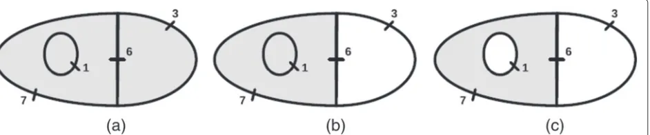
5 ORFC
Differently from RFC, the definitions of ORFC based on paths and based on cuts in the digraph lead to different results (Figures 3a,b). The different obtained algorithms will be denoted as Ain,ORFC and Aout,ORFC for the path-based definition andAin,ORFCQ andAout,ORFCQ for the cut-based definition.
5.1 ORFC definition by reverse connectivity functions Based on the previous works [22,23], we consider the following new connectivity function in digraphs:
Figure 3Example of the different ORFC definitions.(a)ORFC by reverse connectivity functions, with orientation from dark to bright pixels (Ain,ORFC).
(b)ORFC as a directed cut in the digraph (Ain,Q
ORFC).(c)The region of seed robustness (core) ofA in,Q ORFC.
fminS(a) =
wmax+1 ifa∈S
−∞ otherwise
fminS(πa· a,b) = min{fminS(πa),w(b,a)}
whereb,ais an anti-parallel arc.
Note thatfminS is a smooth function, and therefore,Vo
andVb are optimum connectivity maps. These two con-nectivity maps are generated by executing the IFT with anti-parallel connectivity functions:
Vo(a)= max πa∈(G,a)
{f So
min(πa)} (9)
Vb(a)= max πa∈(G,a)
{f Sb
min(πa)} (10)
Following the same key idea from [22] (i.e., to con-sider reversed connectivity functions for one of the seed sets), we have the following natural definition for ORFC: The segmentationAout,ORFC(So,Sb) favoring
transi-tions from bright to dark pixels is obtained by comparing the connectivity mapsVo(a) and Vb(a), such that each
pixela ∈ V is labeled as belonging to the object only if Vo(a) >Vb(a).
Aout,ORFC(So,Sb)=χO: O= {a∈V:Vo(a) >Vb(a)}
(11)
The segmentation AinORFC,(So,Sb) favoring transitions
from dark to bright pixels is obtained by comparing the connectivity mapsVo(a)andVb(a), such that each pixel
a∈Vis labeled as belonging to the object only ifVo(a) >
Vb(a).
Ain,ORFC(So,Sb)=χO:O= {a∈V:Vo(a) >Vb(a)}
(12)
Note that although this ORFC version is based on opti-mum connectivity maps, its practical results have undesir-able characteristics, such as the presence of disconnected regions and high false-positive rates, leading to unsatisfac-tory results (Figure 3a).
5.2 ORFC as a directed cut in the digraph
Given that the previous ORFC definition (Section 5.1) presents undesirable results, in this section, we present an alternative definition supported by a graph cut optimal-ity criterion, which is motivated by the definitions from Section 3.2.
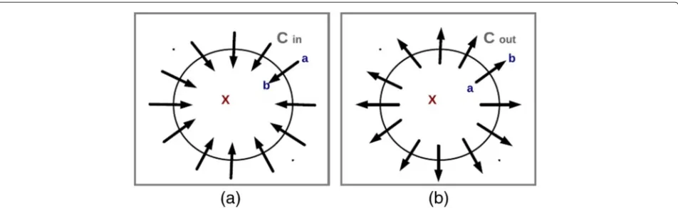
Differently from Section 3.2, in the case of directed graphs, we have two possible sets of cuts (Figure 4):
Cout(x)= {a,b ∈E:x(a)=1∧x(b)=0} (13)
Cin(x)= {a,b ∈E:x(a)=0∧x(b)=1} (14) So we have two possible formulations for the energy functional of theε∞-minimizing problem.
εout
∞ (x)=a,bmax∈Cout(x)w(a,b) (15)
εin
∞(x)= max
a,b∈Cin(x)w(a,b) (16)
Letεout∞↓ be the minimum value of the energy εout∞(x), that is:
εout
∞↓=min{εout∞ (x):x∈X(So,Sb)} (17)
Similarly, forεin∞(x), we have:
εin
∞↓=min{εin∞(x):x∈X(So,Sb)} (18)
Figure 4The two possible sets of cuts. The inner and outer cuts for a candidate object showing the input and output arcs(a,b).
Xout
∞ (So,Sb)=
x∈X(So,Sb):ε∞out(x)=ε∞↓out
(19)
Xin
∞(So,Sb)=
x∈X(So,Sb):εin∞(x)=ε∞↓in
(20)
The ORFC algorithms on digraphs have the following definitions based on cut in graph:
For the outer cut ‘out’ with one internal seeds1,
Aout,ORFCQ({s1},Sb)=χO∈X∞out({s1},Sb):|O|
=min{|P|:χP ∈X∞out({s1},Sb)}
(21)
and in the case of multiple internal seeds,
Aout,ORFCQ(So,Sb)=χO:O=
⎡
⎣
si∈So
P:χP=Aout,ORFCQ({si},Sb)
⎤ ⎦
(22)
For the inner cut ‘in’ with one internal seeds1,
Ain,ORFCQ ({s1},Sb)=χO∈X∞in({s1},Sb):|O|
=min{|P|:χP ∈X∞in({s1},Sb)}
(23)
and in the case of multiple internal seeds,
AinORFC,Q (So,Sb)=χO:O=
⎡
⎣
si∈So
P:χP=Ain,ORFCQ ({si},Sb)
⎤ ⎦
(24)
5.3 ORFC algorithm based on graph cut
In order to show the proposed algorithms, we need the following definition:
Definition 1 (Directed connected component).For a
given vertexxof a digraphG, thedirected connected com-ponent of basepoint x is the set, denoted by DCCG(x),
of all the successors ofxinG(i.e., all the nodes that are reachable from vertexxby some path).
Algorithm 1:
Algorithm to computeAin,ORFCQ ({si},Sb):
1. Compute the value of the mapVb(si)for the functionfSb
min.
2. Remove from the digraphG all arcs with weight≤εin∞↓=Vb(si), obtaining a new digraphG≤.
3. Assign to the object the pixels that belong to the directed connected component of basepointsiin the transpose graph of
G≤(i.e.,AinORFC,Q ({si},Sb)=χO:O= DCCGT
≤(si)).
Figure 5 illustrates the steps of Algorithm 1.
Algorithm 2:
Algorithm to computeAout,ORFCQ({si},Sb):
1. Compute the value of the mapVb(si)for the functionf Sb
min.
2. Remove from the digraphG all arcs with weight≤εout∞↓=Vb(si), obtaining a new digraphG≤.
3. Assign to the object the pixels that belong to the directed connected component of basepointsiin the graphG≤(i.e.,
AoutORFC,Q({si},Sb)=χO: O=DCCG≤(si)).
To prove the correctness of the above algorithms, we need the following lemma:
Lemma 1.For a given weighted digraph G, and sets of
seeds Soand Sb, such that So = {si}, we have thatε∞↓in =
Figure 5AlgorithmAin,ORFCQ (So= {si},Sb).(a)Image as a digraph.(b)Initialization of IFT with background seedSbfor computing the connectivity valueVb(si)using the connectivity functionfminSb.(c)Result of Step 1: The valueVb(si)=1 is computed by the IFT.(d)Step 2: The graphG≤.(e,f)
Step 3: The transpose graph ofG≤and finally, the object’s pixels from the DCC.
Figure 7AlgorithmAout,Q
ORFC+GC(So,Sb).(a)Input image with seedsSoandSb.(b)P:χP=Aout,ORFCQ(So,Sb).(c)Q:χQ=Ain,ORFCQ(Sb,So).(d)AoutOGC(P,Q).
Proof. We will prove Lemma 1 forε∞↓in =Vb(si), but the
caseεout∞↓ =Vb(si)has an essentially identical proof. The
proof is based on the following statement: (1) For the given strongly connected digraphG, if we remove all arcsa,b, such that w(a,b) < ε∞↓in , we then obtain a new digraph Gwhere there still exists a path fromSbtosi(i.e.,∃πtsi wheret∈Sb).
This statement can be proven by contraction. Let T be the set of pixels reachable from Sb in G (i.e., T =
x∈SbDCCG(x)). If there is no path fromSbtosi inG , then we have thatsi ∈/ T. Therefore, we have a partition
of the vertices into two disjoint sets T and V\T. Note that its corresponding cutting arcsa,b ∈ Cin(χV/T)all
have w(a,b) < ε∞↓in in G. Consequently, Cin(χV/T) has
a better cut value thanεin∞↓, which is a contradiction by Equation 18.
From statement (1), we may conclude that there is a path fromSbtosi inG, which is composed only by arcs
a,b:w(a,b)≥εin∞↓. Hence, the connectivity valueVb(si)
of an optimum path fromSbtosi(Equation 2) cannot be
lower thanεin∞↓, i.e.,Vb(si)≥εin∞↓(2).
Consider the set of cutting arcsCin(xopt)of an optimum solutionxopt ∈ X∞in({si},Sb). By definition (Equations 16
and 18), we have that w(a,b) ≤ εin∞↓ for all a,b ∈
Cin(xopt). An optimum path πSbsi, fromSb tosi, must necessarily pass through some arc ofCin(xopt). So its con-nectivity valuefSb
min(πSbsi) = Vb(si) cannot be greater thanεin∞↓, i.e.,Vb(si)≤εin∞↓(3).
From the above conditions (2) and (3), we may conclude that the only valid configuration isVb(si)=ε∞↓in .
For the sake of simplicity, we will only discuss here the proof of correctness of theAin,ORFCQ ({si},Sb)algorithm,
in terms of Equation 23, where s1 = si and εin∞↓ =
Vb(si) (Lemma 1). The algorithm forAORFCout,Q({si},Sb)has
an essentially identical proof.
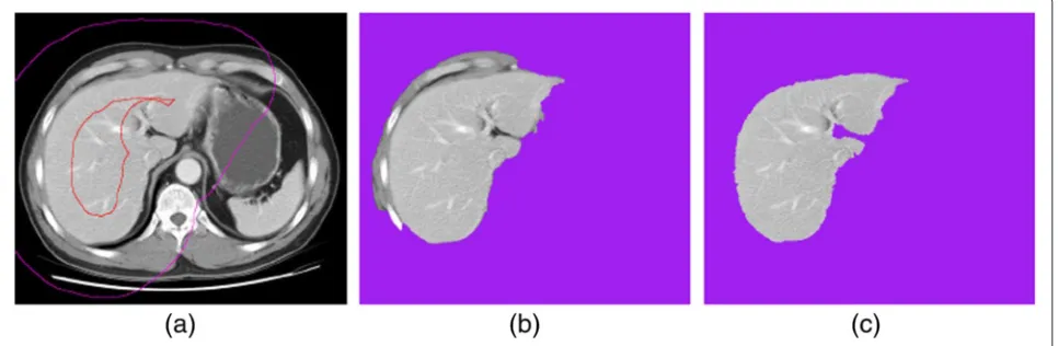
Figure 8Example result by OIFT and ORFC.(a)A CT slice image of the liver with seeds obtained by eroding and dilating the true segmentation.
First, we need to prove that the characteristic function
χO of O = DCCGT
≤(si) is an optimum solution in
Xin
∞({si},Sb). Note that, in the digraphGT≤, there are no
arcs from pixels in DCCGT
≤(si)to pixels inV\DCCGT≤(si); otherwise, the list of successors of si in GT≤, given by DCCGT
≤(si), would not be complete. These arcs were
removed in Step 2 of the Ain,ORFCQ ({si},Sb) algorithm and,
therefore, have no values greater thanεin
∞↓, so the char-acteristic function of DCCGT
≤(si) must be an optimum solution inX∞in({si},Sb).
The other conditions in Equation 23 force
Ain,ORFCQ ({si},Sb) to constitute the smallest object in Xin
∞({si},Sb). Note that any object composed by a set
of pixels T, such that there are arcs from pixels in T to pixels inV\T in the digraphGT≤, cannot be an optimum solution in Xin
∞({si},Sb) because these arcs have
corre-sponding anti-parallel arcs inG≤, pointing toward object pixels, with values greater thanεin∞↓, leading to a worse inner cut. Since all proper subsets of DCCGT
≤(si)still have
some outgoing arcs in the digraphGT≤and, consequently, incoming arcs inG≤, we have that they are not optimum. Therefore, DCCGT
≤(si)is the smallest optimum solution. To solve the case ofAin,ORFCQ (So,Sb)with multiple
inter-nal seeds, according to Equation 24, we need to repeat the execution of Algorithm 1 for each internal seed. How-ever, the following proposition applies in the case of Ain,ORFCQ (So,Sb):
Proposition 1. For a given digraph G = V,E,w
and seed si ∈ So, consider the residual digraph Gsi = G≤ = V,{a,b ∈ E: w(a,b) > Vb(si)},w (step 2 of
Algorithm 1). For any arbitrary seeds s1∈Soand s2∈So,
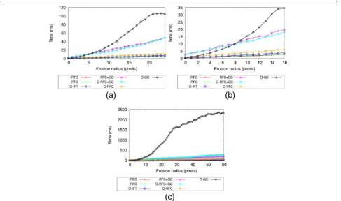
Figure 11 The running time curves for the 2D datasets. The computational time using non-equally eroded-dilated seeds, for segmenting:
(a)calcaneus,(b)talus, and(c)liver.
if Vb(s1)≤Vb(s2)and s2∈DCCGT
s1(s1), then we have that DCCGT
s2(s2)⊂DCCGTs1(s1).
If we sort the seeds si in So according to theirVb(si)
values, then we can process the seeds in increasing order of values, allowing us to avoid the reprocessing of pixels by skipping the seeds that were already assigned to the object, greatly improving the running time.
One important thing to note is that ORFC encompasses RFC as a particular case whenever the parameterαis set to zero.
6 Hybrid segmentation: ORFC and graph cut In this section, we follow the same key ideas from [29], which proposes a hybrid approach combining the strengths of relative fuzzy connectedness and min-cut/max-flow algorithm.
The GC natively supports the soft constraint of bound-ary polarity and will be denoted as oriented graph cut (OGC). It (AoutOGC(So,Sb)) solves theε1-minimization
problem by considering the arcs that limit the flow from the source to the sink and consequently minimizes the sum of the arcs pointing from object to background pix-els (i.e., the outer cut) [11]. The minimization of the sum
of the arcs of the inner cut (AinOGC(So,Sb)) can be obtained
by inverting the source and sink nodes or by reversing all arcs by computing GC over the graph’s transposeGT.
Basically, by considering in [29] a directed weighted graph, with ORFC in place of RFC, we have the ORFC+GC hybrid approach (Figure 6) as follows:
Algorithm 3:
Algorithm to computeAin,ORFC+GCQ (So,Sb):
1. ComputeP:χP =AORFCin,Q (So,Sb). 2. ComputeQ: χQ=AORFCout,Q(Sb,So). 3. Compute and returnAinOGC(P,Q).
Algorithm 4:
Algorithm to computeAout,ORFC+GCQ (So,Sb):
1. ComputeP:χP =AORFCout,Q(So,Sb). 2. ComputeQ: χQ=AORFCin,Q (Sb,So). 3. Compute and returnAoutOGC(P,Q).
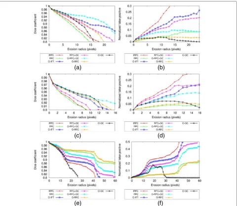
7 Experimental results
In the first experiment, we used 40 slice images from real MR images of the foot. We performed the segmenta-tion of the bones calcaneus and talus for all the methods (IRFC [9], RFC [26], OIFT [23], RFC+GC [29], OGC [11] -the graph cut with boundary polarity, ORFC, and -the pro-posed hybrid method ORFC+GC), for different seed sets automatically obtained by eroding and dilating the ground truth at different radius values. By varying the radius value, we can repeat the segmentation for different seed sets and trace accuracy curves using the dice coefficient of similarity and error curves of false positive (normal-ized by the object size). However, in order to generate a more challenging situation, we considered a larger radius of dilation for the external seeds (twice the value of the inner radius), resulting in an asymmetrical arrangement of seeds. In the second experiment, 40 slice images from CT thoracic studies of 10 subjects were used to segment the liver following the same procedure for seed selec-tion (Figure 8). In all cases, the ground truth data was obtained from an expert of the Radiology Department at the University of Pennsylvania.
Several different procedures can be adopted for δ(a,b)[34,35]. For example, Figures 3 and 9 show some results for user-selected markers using the image-based weight assignment from [36]. For the sake of simplicity,
in the quantitative experiments, we adopted the weight assignment δ(a,b) = K − |G(a) + G(b)|, where G(a) denotes the gradient magnitude of the Sobel operator. In Equation 8,α could be in the range of [ 0, 1], we consid-eredα = 0.5 in all experiments involving OIFT, OGC, ORFC, and ORFC+GC andα = 0.0 in the case of undi-rected approaches. The valueα = 0.5 is the default value adopted in experimental results [22,23], which is a more well balanced configuration. For low values (α ≈ 0.0), the oriented methods (e.g., ORFC) degenerate into their counterpart undirected approaches (e.g., RFC), and for high values, the oriented methods may become more sen-sitive to noise. We usedAin,ORFCQ for the foot bones, since they present transitions from dark to bright pixels and Aout,ORFCQ for the liver, since it has the opposite orientation.
Figure 10 shows the accuracy and error curves, and Figure 11 shows the running time curves for all the meth-ods. Since the considered objects are not expected to have holes, we considered a post-processing by closing of holes (CoH) [37] for RFC and ORFC. Indeed, RFC is known to potentially exclude regions inside the object that are surrounded by strong edges. Note that its oriented counterpart method, ORFC, also inherits this property.
In general, the results show that ORFC can achieve higher accuracy values than RFC, with low false positive errors. Hence, it could be combined with other methods in
Figure 14The running time curves for the 3D datasets. The computational time using non-equally eroded-dilated seeds, for segmenting:
(a)cerebellum dataset and(b)skull stripping dataset.
powerful hybrid approaches. Indeed, the hybrid approach ORFC+GC showed the best results for the calcaneus bone, being more robust than the graph cut with respect to the seed choice. OGC presents a drop of accuracy for higher radius values due to the known ‘shrinking problem’ of graph cut. ORFC presented the best results for the liver segmentation, taking advantage of its homogeneous inte-rior. For the talus, ORFC showed a similar accuracy than ORFC+GC, but with a lower false positive rate and being less time-consuming.
We also repeated the experiments using two three-dimensional datasets. In the former case, a MRI-T1 dataset of the human brain was used to segment the cere-bellum. The images were taken from 20 normal subjects from both genders, in the age range from 16 to 49 years. The images were acquired with a 2T Elscint scanner and at a voxel size of 0.98×0.98×1.00 mm3. The cerebellum is connected to the rest of the brain through the brain stem and through its top due to partial volume. The absence of a clear boundary between these structures poses a signif-icant challenge for segmentation. For the second dataset, we considered a skull stripping task (Figure 12) (i.e., to eliminate background, bones, eyes, skin, and blood ves-sels) using ten 3 Tesla MRI-T1 images, that include the head and, at least, a small portion of the neck of male and female adults with normal brains.
Figures 13 and 14 show the experimental curves. The RFC and ORFC methods performed poorly on these datasets due to the lack of a clear contrast between the structures. Nevertheless, the hybrid approach ORFC+GC showed the overall best results, demonstrating the impor-tance of hybrid methods, and making clear that, even in these cases, ORFC can help to improve the graph cut delineation and to reduce its running time.
8 Conclusions
In this paper, we introduced the ORFC technique and showed that it can effectively exploit the boundary
polarity improving the results in relation to its predeces-sor RFC. We also presented a powerful hybrid approach, which outperforms the previous works [29,30]. As future work, we plan to investigate the theoretical relations between ORFC and OIFT, the usage of shape constraints in the ORFC (similar to what was done in [25]), and to combine the proposed methods with fuzzy object mod-els[38-41] in order to get a fully automatic segmentation result.
Competing interests
The authors declare that they have no competing interests.
Acknowledgements
The authors thank CNPq (305381/2012-1, 486083/2013-6, FINEP 1266/13), FAPESP grant # 2011/50761-2, CNPq, CAPES, NAP eScience - PRP - USP, and Dr. J. K. Udupa (MIPG-UPENN) for the images.
Received: 6 January 2015 Accepted: 31 March 2015
References
1. J Deng, N Ding, Y Jia, A Frome, K Murphy, S Bengio, Y Li, H Neven, H Adam, inComputer Vision - ECCV 2014.Lecture Notes in Computer Science, ed. by D Fleet, T Pajdla, B Schiele, and T Tuytelaars. Large-scale object classification using label relation graphs, vol. 8689 (Springer, Zurich, Switzerland, 2014), pp. 48–64
2. KS Camilus, VK Govindan, A review on graph based segmentation. Intl. J. Image, Graphics Signal Process.4(5), 1–13 (2012)
3. C Vehlow, T Reinhardt, D Weiskopf, Visualizing fuzzy overlapping communities in networks. Vis. Comput. Graphics, IEEE Trans.19(12), 2486–2495 (2013). doi:10.1109/TVCG.2013.232
4. O Chum, J Matas, Large-scale discovery of spatially related images. Pattern Anal. Mach. Intell. IEEE Trans.32(2), 371–377 (2010). doi:10.1109/TPAMI.2009.166
5. O Lézoray, L Grady,Image processing and analysis with graphs: theory and practice. (CRC Press, California, USA, 2012)
6. J Cousty, G Bertrand, L Najman, M Couprie, Watershed cuts: thinnings, shortest path forests, and topological watersheds. IEEE Trans. Pattern Anal. Mach. Intell.32, 925–939 (2010). doi:10.1109/TPAMI.2009.71 7. RA Lotufo, AX Falcão, F Zampirolli, inProceedings of the XV Brazilian
Symposium on Computer Graphics and Image Processing. IFT-watershed from gray-scale marker, (2002), pp. 146–152.
doi:10.1109/SIBGRA.2002.1167137
9. KC Ciesielski, JK Udupa, PK Saha, Y Zhuge, Iterative relative fuzzy connectedness for multiple objects with multiple seeds. Comput. Vis. Image Underst.107(3), 160–182 (2007)
10. R Audigier, RA Lotufo, inProceedings of the XX Brazilian Symposium on Computer Graphics and Image Processing (SIBGRAPI). Seed-relative segmentation robustness of watershed and fuzzy connectedness approaches (IEEE CPS Belo Horizonte, MG, 2007), pp. 61–68 11. Y Boykov, G Funka-Lea, Graph cuts and efficient N-D image
segmentation. Intl. J. Comp. Vis.70(2), 109–131 (2006)
12. X Bai, G Sapiro, inProc. of the IEEE Intl. Conf. on Image Processing. Distance cut: interactive segmentation and matting of images and videos, vol. 2 (IEEE Computer Society, Washington D.C., 2007), pp. 249–252 13. AX Falcão, J Stolfi, RA Lotufo, The image foresting transform: theory,
algorithms, and applications. IEEE Trans. Pattern Anal. Mach. Intell.26(1), 19–29 (2004)
14. V Vezhnevets, V Konouchine, inProc. Graphicon. "GrowCut" - interactive multi-label N-D image segmentation by cellular automata (Moscow State University, Moscow, 2005), pp. 150–156
15. AK Sinop, L Grady, inProc. of the 11th Intl. Conf. on Computer Vision. A seeded image segmentation framework unifying graph cuts and random walker which yields a new algorithm (IEEE, Washington D.C., 2007), pp. 1–8 16. PAV Miranda, AX Falcão, inXXIV Conference on Graphics, Patterns and
Images. Elucidating the relations among seeded image segmentation methods and their possible extensions (Maceió, AL, 2011), pp. 289–296. doi:10.1109/SIBGRAPI.2011.13
17. KC Ciesielski, JK Udupa, AX Falcão, PAV Miranda, Fuzzy connectedness image segmentation in graph cut formulation: a linear-time algorithm and a comparative analysis. J. Math. Imaging Vis.44(3), 375–398 (2012) 18. C Couprie, L Grady, L Najman, H Talbot, Power watersheds: a unifying
graph-based optimization framework. IEEE Trans. Pattern Anal. Mach. Intell.99(7), 1384–1399 (2010). doi:10.1109/TPAMI.2010.200
19. PAV Miranda, AX Falcão, Links between image segmentation based on optimum-path forest and minimum cut in graph. J. Math. Imaging Vis. 35(2), 128–142 (2009)
20. KC Ciesielski, JK Udupa, AX Falcão, PAV Miranda, inProc. of SPIE on Medical Imaging: Image Processing. A unifying graph-cut image segmentation framework: algorithms it encompasses and equivalences among them, vol. 8314, (2012). doi:10.1117/12.911810
21. Y Boykov, V Kolmogorov, An experimental comparison of min-cut/max-flow algorithms for energy minimization in vision. IEEE Trans. Pattern Anal. Mach. Intell.26(9), 1124–1137 (2004)
22. PAV Miranda, LAC Mansilla, Oriented image foresting transform segmentation by seed competition. IEEE Trans. Image Process.23(1), 389–398 (2014)
23. LAC Mansilla, PAV Miranda, in18th Intl. Conf. on Digital Signal Processing, Greece. Image segmentation by oriented image foresting transform: handling ties and colored images (IEEE Computer Society, Washington D.C., 2013), pp. 1–6
24. D Singaraju, L Grady, R Vidal, inIntl. Conf. on Computer Vision and Pattern Recognition. Interactive image segmentation via minimization of quadratic energies on directed graphs (IEEE, Washington D.C., 2008), pp. 1–8 25. LAC Mansilla, PAV Miranda, in15th International Conference on Computer
Analysis of Images and Patterns (CAIP),vol. 8047. York, UK. Image segmentation by oriented image foresting transform with geodesic star convexity (Springer, Berlin Heidelberg, 2013), pp. 572–579
26. PK Saha, JK Udupa, Relative fuzzy connectedness among multiple objects: theory, algorithms, and applications in image segmentation. Comp. Vision Image Underst.82(1), 42–56 (2001)
27. PAV Miranda, AX Falcão, GCS Ruppert, FAM Cappabianco, inProc. of the IEEE Intl. Symp. on Biomedical Imaging (ISBI). How to fix any 3D segmentation interactively via image foresting transform and its use in MRI brain segmentation (IEEE Computer Society, Washington D.C., 2011), pp. 2031–2035
28. PAV Miranda, AX Falcão, G Ruppert, in23rd SIBGRAPI: Conf. on Graphics, Patterns and Images. How to complete any segmentation process interactively via image foresting transform (IEEE Computer Society, Washington D.C, 2010), pp. 309–316
29. KC Ciesielski, PAV Miranda, AX Falcão, JK Udupa, Joint graph cut and relative fuzzy connectedness image segmentation algorithm. Med. Image Anal. (MEDIA).17(8), 1046–1057 (2013)
30. KC Ciesielski, PAV Miranda, JK Udupa, AX Falcã, inProc. of the International Conference on Image Processing. Image segmentation by combining the strengths of relative fuzzy connectedness and graph cut (IEEE, Orlando, Florida, USA, 2012), pp. 2005–2008
31. HHC Bejar, PAV Miranda, inXXVII SIBGRAPI - Conference on Graphics, Patterns and Images. Oriented relative fuzzy connectedness: theory, algorithms, and applications in image segmentation (IEEE Computer Society, Rio de Janeiro, Brazil, 2014), pp. 304–311
32. JK Udupa, PK Saha, RA Lotufo, Relative fuzzy connectedness and object definition: theory, algorithms, and applications in image segmentation. IEEE Trans. Pattern Anal. Mach. Intell.24, 1485–1500 (2002)
33. K Ciesielski, J Udupa, inBiomedical Image Processing.Biological and Medical Physics, Biomedical Engineering, ed. by TM Deserno.
Region-based segmentation: fuzzy connectedness, graph cut and related algorithms (Springer, Berlin, Germany, 2011), pp. 251–278
34. KC Ciesielski, JK Udupa, Affinity functions in fuzzy connectedness based image segmentation I: equivalence of affinities. Comput. Vision Image Underst.114(1), 146–154 (2010)
35. KC Ciesielski, JK Udupa, Affinity functions in fuzzy connectedness based image segmentation II: defining and recognizing truly novel affinities. Comput. Vision Image Underst.114(1), 155–166 (2010)
36. PAV Miranda, AX Falcão, JK Udupa, Synergistic arc-weight estimation for interactive image segmentation using graphs. Comput. Vision Image Underst.114(1), 85–99 (2010)
37. AX Falcão, BS da Cunha, RA Lotufo, inProceedings of SPIE on Medical Imaging. Design of connected operators using the image foresting transform, vol. 4322 (SPIE, Bellingham, 2001), pp. 468–479
38. JK Udupa, D Odhner, L Zhao, Y Tong, MMS Matsumoto, KC Ciesielski, AX Falcao, P Vaideeswaran, V Ciesielski, B Saboury, S Mohammadianrasanani, S Sin, R Arens, DA Torigian, Body-wide hierarchical fuzzy modeling, recognition, and delineation of anatomy in medical images. Med. Image. Anal.18(5), 752–771 (2014). doi:10.1016/j.media.2014.04.003
39. JK Udupa, D Odhner, AX Falcã, KC Ciesielski, PAV Miranda, S Mishra, GJ Grevera, B Saboury, DA Torigian, inProceedings of SPIE on Medical Imaging: Image-Guided Procedures, Robotic Interventions, and Modeling. Automatic anatomy recognition via fuzzy object models, vol. 8316 (SPIE, San Diego, California, USA, 2012)
40. PAV Miranda, AX Falcão, JK Udupa, inProceedings of the IEEE International Symposium on Biomedical Imaging (ISBI). Cloud bank: a multiple clouds model and its use in MR brain image segmentation (IEEE, Boston, MA, 2009), pp. 506–509
41. PAV Miranda, AX Falcão, JK Udupa, inProceedings of the IEEE International Symposium on Biomedical Imaging (ISBI).CLOUDS: a model for synergistic image segmentation (Paris, France, 2008), pp. 209–212
Submit your manuscript to a
journal and benefi t from:
7Convenient online submission
7Rigorous peer review
7Immediate publication on acceptance
7Open access: articles freely available online
7High visibility within the fi eld
7Retaining the copyright to your article

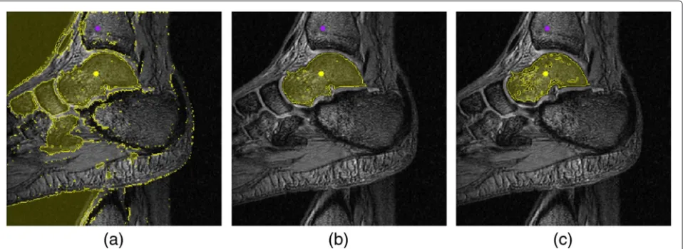
![Figure 6 An example result of ORFC+GC. The segmentation of the wrist by: (a) IRFC [9], (b) OIFT [22], (c) RFC+GC [29], and (d) ORFC+GC.](https://thumb-us.123doks.com/thumbv2/123dok_us/910705.1588848/7.595.57.548.87.383/figure-example-result-orfc-segmentation-wrist-irfc-orfc.webp)
![Figure 9 Example results for the different methods.weight assignment from [36]. (a) A talus bone in an MRI slice of a foot with user-selected markers](https://thumb-us.123doks.com/thumbv2/123dok_us/910705.1588848/9.595.61.542.155.698/figure-example-results-different-methods-assignment-selected-markers.webp)