Solving the dynamic equations of a 3-PRS Parallel Manipulator for efficient model-based designs

www.mech-sci.net/7/9/2016/ doi:10.5194/ms-7-9-2016

© Author(s) 2016. CC Attribution 3.0 License.

Solving the dynamic equations of a 3-PRS Parallel

Manipulator for efficient model-based designs

M. Díaz-Rodríguez1, J. A. Carretero2, and R. Bautista-Quintero2,3

1_{Departamento de Tecnología y Diseño, Facultad de Ingeniería, Universidad de los Andes,} Mérida, 5101, Venezuela

2_{Department of Mechanical Engineering, University of New Brunswick, Fredericton, NB, E3A 5A3, Canada} 3_{Departamento de Ingeniería Mecánica, Instituto Tecnológico de Culiacán, Sinaloa, 80220, Mexico}

Correspondence to: M. Díaz-Rodríguez ([email protected])

Received: 6 December 2014 – Revised: 14 October 2015 – Accepted: 14 December 2015 – Published: 18 January 2016

Abstract. Introduction of parallel manipulator systems for different applications areas has influenced many researchers to develop techniques for obtaining accurate and computational efficient inverse dynamic mod-els. Some subject areas make use of these models, such as, optimal design, parameter identification, model based control and even actuation redundancy approaches. In this context, by revisiting some of the current computationally-efficient solutions for obtaining the inverse dynamic model of parallel manipulators, this paper compares three different methods for inverse dynamic modelling of a general, lower mobility, 3-PRS parallel manipulator. The first method obtains the inverse dynamic model by describing the manipulator as three open kinematic chains. Then, vector-loop closure constraints are introduced for obtaining the relationship between the dynamics of the open kinematic chains (such as a serial robot) and the closed chains (such as a parallel robot). The second method exploits certain characteristics of parallel manipulators such that the platform and the links are considered as independent subsystems. The proposed third method is similar to the second method but it uses a different Jacobian matrix formulation in order to reduce computational complexity. Analysis of these nu-merical formulations will provide fundamental software support for efficient model-based designs. In addition, computational cost reduction presented in this paper can also be an effective guideline for optimal design of this type of manipulator and for real-time embedded control.

1 Introduction

Seminal research in Parallel Manipulators (PMs) described architectures of 6 degrees of freedom (DOF) which are mainly used to perform industrial tasks. Nevertheless, not all applications (e.g., commercial, space exploration, enter-tainment or even industrial) require full 6-DOF capabilities, thus, cost-effective PMs with less than 6 DOF (i.e., lower-mobility) have been developed. One such architecture is the 3-PRS manipulator which has a platform and a fixed base connected through three identical sets of links and joints (i.e., legs). Each leg has a slider attached to the base by an actu-ated prismatic joint (P), a coupler connected to the slider by a passive rotational joint (R) and to the platform by a pas-sive spherical joint (S). The 3-PRS manipulator was first

Lagrangian formulations allowed to develop the inverse dynamics model of the 3-PRS manipulator (Li and Xu, 2004). The formulation uses the Lagrange multiplier to in-clude the constraints forces that lead to a modelling approach not only intricate but also computationally complex. Li and Xu (2004) applied the Principle of Virtual Work (PVW), but they simplify the dynamics of the coupler link by dividing its mass into two portions located at its extremes. Tsai and Yuan (2010) solved the inverse dynamic model along with the reaction forces through a special decomposition of the reaction forces at the joints that connect the leg with the plat-form. A similar approach was used in Yuan and Tsai (2014) for solving direct dynamics including friction effect. How-ever, the later approach considers the calculation of reaction forces which are may be needed for structural design of a ma-nipulator but its computation increases computational com-plexity which is unnecessary for parameter identification or model-based control. Staicu (2012) analyses and compares the power consumption of the 3-PRS vs. the 3-PRS configu-ration using the PVW with recursive modelling. The method obtains the Jacobian by differentiating the vector loop equa-tion. Carbonari et al. (2013) solved the inverse dynamics of a 3-DOF parallel manipulator via screw theory and the PVW. On the other hand, the 3-RPS manipulator presents simi-lar characteristics to the 3-PRS manipulator, in this respect, Mata et al. (2008) implement recursive velocity equations used in serial manipulator analysis to find the Jacobian of the manipulator for the inverse dynamic modelling, and Ibrahim and Khalil (2007) exploit architectural characteristics of the 3-RPS to give a closed form solution for the inverse and di-rect dynamics modelling.

The inherent complexity of the dynamic models lies on the way the system is modelled and how the Jacobian matrix is put forward. In this context, this paper compares the compu-tational number of operation of three formulations for inverse dynamic modelling of a 3-PRS. The first formulation applies the general solution of PMs dynamic modelling proposed in Khalil and Ibrahim (2007). The second method considers the manipulator as a set of open kinematic chains and finds the Jacobian in joint space coordinates by taking into account the vector loop constraints at the split joints (Mata et al., 2008). The third method relies on the modelling approach originally presented in Li and Xu (2004).

The ultimate goal of contrasting these numerical formula-tions is focused on supporting the implementation of emerg-ing model-based designs which not only depends of the dis-crete inverse dynamic model but also the numerical finite realization in a given computational platform (Williamson, 1991). In fact, software architecture, for model based con-trol (Díaz-Rodríguez et al., 2013), relies on minimizing com-putational task timing commonly constrained by fast sam-pling periods (Goodwin et al., 1992). Similarly, in other ap-plications, such parameter identification (Mata et al., 2008), and internal redundancy (Parsa et al., 2013) few papers have focused on revisiting and comparing

computationally-inexpensive methods in order to obtain the dynamic model of the 3-PRS configuration for cost-effective real-time appli-cations.

To this end, this paper is organized as follows: Sect. 2 presents in general terms how the dynamic model for a paral-lel manipulator is developed for the three approaches inves-tigated in this paper. Section 3 presents the implementation of the approaches for solving the dynamics problem of a 3-PRS spatial parallel manipulator. Section 4 summarizes and discusses the complexity and the computational load of these three formulations. Finally, the conclusions are drawn.

2 Development of the dynamic models

The dynamic model of a closed chain mechanical system such as a parallel manipulator can be obtained by virtually cutting or splitting the manipulator at one or more of its joints until the complete dynamic model of a tree-like system with several open chains is obtained. Newton–Euler formulations are then used for solving the dynamics of each serial chain. Finally, constraint equations obtained by means of the La-grange Multipliers are incorporated to include the necessary forces at the splitting points as to ensure the kinematic chains remain closed. On the other hand, the Lagrangian approach can be applied by using the Lagrange equation with respect to a minimum set of generalized coordinates. Yiu et al. (2001) showed that either application of Lagrange Equation or tree-like system analysis are equivalent to one another and lead to the same set of equations when applied to a parallel ma-nipulator. Moreover, similar results were obtained by Murray and Lovell (1989) using the D’Alembert’s principle and the principle of virtual work.

Regardless, of the dynamics equation (Newton–Euler, La-grange or Principle of Virtual Work) used for developing the model, the dynamics of closed chain system can be written as:

τ=GTh. (1)

This equation establishes that the generalized forces corre-sponding to an open chain system (h) are related to the ac-tuated forces of a closed chain system (τ) by a linear trans-formation GT. This linear transformation is based on the Jacobian matrix. Thus, the dynamics equation of a parallel manipulator essentially relies on finding the Jacobian matrix that relate the passive generalized coordinates to the actuated ones.

differences in the number of algebraic operations to compute each. The objective of this work is mostly revisiting these approaches to find the cost-effectiveness of each when solv-ing the inverse dynamics through an example. This is of par-ticular interest as inexpensive computer models are essential when adaptive control algorithms are used to control manip-ulator at fast update rates. For instance, in the fields of param-eter identification and actuation redundancy, a fast estimation of the inverse model implies cost-effectiveness for real-time applications.

2.1 Dynamics considering the legs and platform as subsystems

This approach is based on the general formulation for mod-elling parallel manipulators presented by Khalil and Ibrahim (2007), which is based on the following aspects: (1) the ma-nipulator is split open at the spherical joints so that the mov-ing platform is separated from the legs and (2) the local joint coordinates systems q can be used to develop the dynamic equations of each leghi while the Cartesian coordinates x

are used to obtain the dynamic equations of the platform

hp. Then, the dynamic equations are combined and projected onto the active joint space as follows:

τ =JT_php+

m X

i=1

_δq˙ i

δq˙a

T

hi, (2)

where Jp is the Jacobian projecting the task space coordi-nates (6 in the general case) to thenactive joint coordinates, whilemis the number of joints for each leg. Likewise,

hp=

"

mpg−mpap

−Ipω˙p−ωp× Ipωp

#

, (3)

wheremp is the mass of the platform, Ipdenotes the iner-tial matrix of the moving platform about its centre of mass,

apstands for the acceleration of the end effector, andωp,ω˙p respectively denote the angular velocity and angular acceler-ation of the platform.

2.1.1 Method I

In order to develop the model in actuated joint space one has to project the passive joint variables to the active ones. That is:

τ =ha_i+JT_php+GTIh p

i, (4)

where indices a and p stand for the active and passive joints, respectively, while GIis al×nmatrix projecting the dynam-ics from the passive to the active joints. Here, l represents the number of passive joints whilenis the number of active joints on each leg.

{O}

l

s

l

Figure 1.Closed chain equation for finding GI.

Equation (4) can be written in the form of Eq. (1). That is:

τ=

I JT_p GT_I 

 

ha_i hp

hp_i 

 =G

T_{h, (5)}

where I is the identity matrix with dimension equal to the degree of freedom of the manipulator.

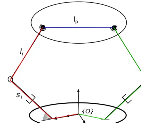
In Eq. (4), matrix GI can be obtained by considering the fact that the distance among spherical joints at the platform is constant due to the rigid body assumption. This distance is calculated based on the norm of the vector obtained by subtracting the position vector identifying the location of the spherical joints. The partial derivatives of each equation with respect to the joints coordinates yields matrix GI. Figure 1 shows how to establish the closed chain equations.

Note that in Eq. (4),hpis a 6×1 vector and, in the partic-ular case of a 3-PRS parallel manipulator,τ is a 3×1 vector. Therefore, matrix Jp is not square and cannot be obtained using previous methods for solving the inverse kinematics of this kind of manipulator. For instance, when developing the inverse dynamics model using the Principle of Virtual Work, Li and Xu (2004) found a 3×3 square matrix Jp. They did so by only considering three of the components of the plat-form inertial forces; they considered those associated with the desired degrees of freedom of the end effector. In Sect. 3 a method obtaining Jpconsidering the 6 components ofhp for the particular case of the 3-PRS manipulator is shown.

2.1.2 Method II

space, and then, project them back to the active joint space so that:

τ =ha_i+J_pThhp+GTIIh p

i i

, (6)

where GIIis al×6 matrix that holds new definition that can be written as follow:

GT_II=JT_v iJ

−T

qi , (7)

where Jviand J −T

qi can be obtained respectively from the di-rect Jacobian Jxand the inverse Jacobian Jq of the

manipu-lator.

Equation (6) can be written in the form of Eq. (1). That is:

τ = h

I JT

p GIIJpT

i 

 

ha_i hp

hp_i 

 =G

T_{h. (8)}

2.2 Dynamics considering the manipulator as open kinematic chains

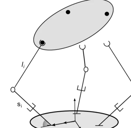
A parallel manipulator can be split open into m−1 joints yieldingmopen chain systems. In this approach the platform is attached to one of the legs, see Fig. 2. Algorithms for ob-taining the dynamics model of serial manipulators may now be applied to obtain the dynamics of each leg.

The cut joints introduce constraint forces, which can be in-cluded into the model by means of the Lagrange multipliers:

τ =hi+Aλi, (9)

where A is the Jacobian that can be found by analysing the constraint equations. Mata et al. (2008) presented a method for the Jacobian matrix by considering the linear velocity at the split joints. The velocities can be computed through the Jacobian analysis of each leg. Then, the velocity obtained at the split joint following each leg are the same. In this approach, recursive modelling of the velocity analysis from conventional serial manipulator methods can be applied for each leg.

Once the Jacobian matrix is found, the Lagrange multi-pliers in Eq. (9) are eliminated by multiplying matrix C, so that, CA=0. One way to find C is by obtaining the natural orthogonal complement of C. On the other hand, the matrix can be found by separating matrix A=0 into the passive and the active joints. That is:

τ =ha+GT_IIIhp, (10) where GIIIhas dimensionsl×nand can be computed as fol-lows:

GIII=A−p1Aa, (11)

where subscripts p and a respectively refer to the passive and active variable terms in Jacobian A. Equation (10) can be

l

s

Figure 2.Several open chains obtained after cutting open the par-allel manipulator.

written in the form of Eq. (1). That is:

τ= I GIII

" ha_i hp_i #

=GTh. (12)

As Eqs. (5), (8) and (12) show, the three methods estab-lish a linear relation between the cut-open model (h) to the original system. The different lies in how matrix GT _and

vec-torhare solved in each model. This is illustrated in the next section for the particular case of a general 3-PRS parallel manipulator.

3 Inverse dynamics of the 3-PRS PM

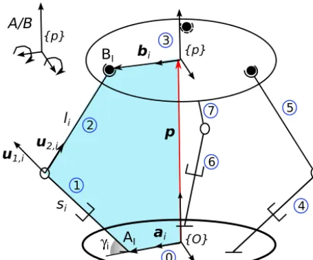
A schematic representation of the 3-PRS PM is shown in Fig. 3 where the 7 moving rigid bodies are shown. There, links 0, 1, and 2 can be seen as 2-DOF serial manipulator with PR joints, also it applies to links 0, 4, and 5 as well as links 0, 6, and 7. The platform is indicated by the number 3. The manipulator is a lower mobility (i.e., less that 6-DOF) spacial PM with 3-DOF. This manipulator holds the charac-teristic of zero torsion at its platform because the three spher-ical joints move in vertspher-ical planes intersecting at a common line (Liu and Bonev, 2008). In addition, the topology of its legs provides 2-DOF of angular rotation (2R) in two axes (A/Baxis, rolling and pitching) and 1-DOF translation (1T) motion (heave) at the end effector.

{p}

{O}

u_1,i u2,i l_i

a_i bi

p

si

gi AI BI 1 2 3 4 7 6 5 0 {p} A/B

Figure 3.Sketch of a general 3-PRS manipulator.

at the platform form an equilateral triangle circumscribed in a circle with centre p and radiusrp. The line of action of

the prismatic joints intersects the baseOxy plane atAi also

forming an equilateral triangle. The distance fromOtoAi is

the base platform radiusrb.

In order to take advantage of the dynamic equation al-gorithms developed for serial manipulators, when modelling the manipulator with leg and platform as subsystem, the joint coordinatesqcan be used to develop the dynamics equations of each leg (Mata et al., 2002). To this end, a local coordi-nate system {Oi,0}is defined at the bottom of legi where the leg meets the based plane. Table 1 lists the Denavit– Hartenberg (D–H) parameters, according to Craig’s notation (Craig, 2005), of each legifrom{Oi,0}up to the location of the axis{Oi,2}at the revolute joint.

The rotation matrixOi,0_{Rocan be found as:}

Oi,0_R O=





−sin (ξi) 0 cos (ξi)

cos (ξi) 0 sin (ξi)

0 1 0



, (13)

whereξ=

0 2/3π 4/3πT.

In addition, the roll-pitch-yaw (α,β andφ) Euler angles represent the orientation of the moving frame {p}with re-spect to the global coordinate system{O}. The rotation ma-trixORpis defined as:

O_R

p=





cαcβ cαsβsφ−sαcφ cαsβcφ+sαsφ

sαcβ sαsβsφ+cαcφ sαsβcφ−cαsφ −sβ cβsφ cβcφ



, (14)

wherec∗=cos (∗) ands∗=sin (∗).

Table 1.D–H parameters for a 3-PRS PM when modelling the ma-nipulator with leg and platform as subsystem.

i θi,1 di,1 ai,1 αi,1 θi,2 di,2 ai,2 αi,2

1 π/2 s1 0 γ1 θ1 0 0 −π/2

2 π/2 s2 0 γ2 θ2 0 0 −π/2

3 π/2 s3 0 γ3 θ3 0 0 −π/2

The task space (x) and joint space (q_i) coordinates are given by:

x=xp yp zp φ β αT, (15)

q=hqT₁ qT₂ qT₃i, (16)

q₁=

s1

θ1

, q₂=

s2

θ2

, and q₃=

s3

θ3

, (17)

wheresi represents the displacement along the axis of the

prismatic jointi, andθithe angle of the link 2 and the axis of

the prismatic jointiin the plane of movement of the legi. The components ofbi with respect to the local coordinate

system{p}are given by:

p_b 1= " _r p 0 0 #

, pb2=



  

−1

2rp √

3 2 rp

0



  

,andpb3=



  

−1

2rp −

√ 3 2 rp 0     (18)

while the components ofai with respect to the global

coor-dinate system{O}are given by:

a1=

  rb 0 0 

,a2=

     −1 2rb √

3 2 rb

0     

,anda3=

     −1 2rb

− √

3 2 rb

0      . (19)

The position problem for the considered PM is not in-cluded in this paper since it can be found in Carretero et al. (2000b), Tsai et al. (2002), Li and Xu (2004), Mata et al. (2008). The following subsections focus on the computation of the Jacobian matrix for the aforementioned approaches.

3.1 Jacobian matrix for Model I

Matrices Jpand G for computing Eq. (4) are found following the approach presented in Li and Xu (2004). The vector loop equation of theith leg can be written as:

p+bi=ai+siu1i+liu2i, (20) whereu1i andu2iare unit vectors,liis the distance between the rotational joint and the spherical joint,bi is the position

each leg. Differentiating Eq. (20) with respect to time and af-ter some algebraic manipulation, the following equation can be obtained:

Jqq˙=Jxx˙ (21)

where:

Jq= 

 

uT₂₁u11 0 0

0 uT

22u12 0

0 0 uT

23u13





 (22)

and

Jx= 

  

uT₂₁ (b1×u21)T

uT₂₂ (b2×u22)T

uT

23 (b3×u23)

T     . (23)

Due to the constraints imposed by the fact that each legs moves on a plane, the following set of equations holds:

xp= −rpsαcβ,

yp= − 1

2rp cαcβ−sαsβsφ−cαcφ

, (24)

tan (α)= sβsφ

/ cφ+cβ

.

From these equations, a 6×3 Jacobian matrix mapping the dependent task space coordinates to the independent ones can be found such that:

˙

xp y˙p z˙p φ˙ β˙ α˙

T =J∗_r

˙

zp φ˙ β˙

T

(25)

It is important to note that x˙=

˙

xp y˙p z˙p ωpx ωyp ωzp T

. In order to apply Eq. (25), one has to find the angular velocity of the platform through the rate of change of the generalised coordinates

˙

α β˙ φ˙T. That is:





ωpx

ωyp

ωzp 

= 



cαcβ −sα 0

sαcβ cα 0 −sβ 0 1     ˙ φ ˙ β ˙ α 

. (26)

After some algebraic manipulation the following equation can be obtained:

Jp=JrJ−c1 (27)

where Jc= h

J−_q1JxJr i

.

The 3×3 matrix GIis found by considering the fact that the distance among spherical joints at the platform is constant due to the rigid body assumption. That is:

l2_p− ||ai+siu1i+liu2i−ai+1−si+1u1i+1

−li+1u2i+1|| =0 (28) withi=1,2,3 and wheni=3,i+1=1.

Thus, by obtaining the partial derivatives of the above set of equation matrix GIcan be written as:

           

δ

θ

˙

δ

s1

˙

δ

θ

˙

δ

s1

˙

δ

θ

˙

δ

s1

˙

δ

θ1

˙

δ

s

˙

δ

θ2

˙

δ

s

˙

δ

θ2

˙

δ

s

˙

δ

θ1

˙

δ

s

˙

δ

θ2

˙

δ

s

˙

δ

θ3

˙

δ

s

˙

           

=X−_p1Xa=GI. (29)

3.2 Jacobian matrix for Model II

Another approach to compute matrices Jpand G is to con-sider that the spherical joints in each leg is constrained to move on a plane normal to the revolute joint. The motion of each leg at pointBi can be found in terms of the joint

co-ordinates. Moreover, it can also be expressed with respect to

Oi,2. Due to the constraints provided by the P–R pair, the third row of the Jacobian matrix consist of zero entries. That is:

i,2_v

Bi= i_Jqq

i, (30)

where

i_J q=





−sin (θi) 0 −cos (θi) li

0 0



. (31)

The linear velocity of the end effector can be related to the linear velocity of pointsBias follows:

i,2_v

Bi=

i_{Jvv= i,2}

RO −i,2RO ORppebi

v, (32)

where

v= vT

p ωTp

T

= vpx vpy vpz ωx ωy ωz T

, eb

stands for the skew symmetric matrix substituting the cross productbi×, and

i,2_R p=



 

−cσisγi+θi −cσicγi+θi sσi −sσisγ1+θi −sσicγ1+θi −cσi

cγ+θi −sγi+θi 0 



. (33)

The first two rows of Eqs. (31) and (32) relate the task space to the joint spaces coordinates. That is:

Jqq˙=Jxv, (34)

where

Jq= 



1_J

q 0 0

0 2Jq 0 0 0 3Jq



Table 2.D–H Parameters for the first leg of the 3-PRS PM when modelling as a three open chains.

j θ1,j d1,1 a1,j α1,j

1 π/2 s1 0 −γ1

2 θ1 0 0 −π/2

3 θ4 l1 0 0

4 θ5 0 0 π/2

5 θ6 0 0 π/2

and,

Jx= 

            

xT1,2_{RO x}T ₋1,2_RO OR

p

peb1

yT1,2_R

O yT −1,2RO_ORppeb1

xT2,2_R

O xT −2,2RO_ORppeb1

yT2,2_{RO y}T ₋2,2_RO OR

p

peb1

xT3,2_R

O xT −3,2ROOR p

peb1

yT3,2RO yT −3,2ROOR p

peb1



            

. (36)

In the above equationsx= 1 0 0T,

y= 0 1 0T, and 0 is a 2×2 zero matrix.

From the above equation, matrix GIIcan be obtained as follows:

J−_q1Jx= 

  

J−_q11Jv1

J−_q21Jv2

J−_q31Jv2



  

(37)

GT_II=h JT_v1J_q1−T(:,2) JT_v2J_q1−T(:,2) JT_v3J_q3−T(:,2)i (38)

where A (:,2) denotes the 2nd column of matrix A.

The Jacobian matrix, relating the task space coordinates

Jr, is found by considering the third column of velocity

equa-tion following each leg and the platform. The Jacobian ma-trix is obtained by following method 2 which is graphically represented in Fig. 4.

3.3 Jacobian matrix for Model III

The inverse dynamic is computed as a function of three open chains which are obtained after disassembling two of the three spherical joints. The platform is attached to one of the legs, and the spherical joint is modelled as three intersecting revolute joints with the three axes mutually perpendicular to one another. Therefore, the chain with the end effector plat-form is modelled by using the set of D–H parameters pre-sented in Table 2. The remaining legs have only sets of two variables which are the same as those presented in Table 1.

One of the advantages of considering the manipulator as tree-like serial chains is that the Jacobian for each leg can

be computed by using well-known recursive modelling from serial manipulator. In this respect, the velocities at the cut joints can be computed through recursive formulation (An-geles, 2002). That is:

Aiq˙i=VBi,i+1 =Ai+1q˙i+1, (39) wherei=1,2,3 and wheni=3,i+1=1, Aiis the Jacobian

matrix for theith leg, andVBi,i+1 is the velocity at the cut

joint connecting legiandi+1.

From Eq. (39) the following equation can be obtained:

Aiq˙i−Ai+1q˙i+1=0. (40) This equation provides a set of three linear systems relating the joint coordinates following each loop. If the set of linear equations is appended together the following equation holds:

X= 



A1 −A2 03×3

03×3 A2 −A3

A1 03×3 −A3



q˙=0. (41)

The relationship between the active and passive coordi-nates can be obtained from Eq. (41) as follows:

GIII=X−p1Xa. (42)

4 Results and discussion

In order to solve the inverse dynamics of the 3-PRS parallel manipulator, each term of Eqs. (4), (6), and (10) are found in closed form by using a Computer Algebra Symbolic (CAS) program, such as Maple. One of the advantages of devel-oping the model in a CAS program relies on the fact that the mathematical operations can be performed symbolically and simplified. In the present case, built-in functions such as

simplifyandcombine(withoption=trig) of Maple programming environment were used to reduce the number of operations for solving each model.

A second advantage of obtaining the model in closed form is that the code can be written automatically forMatlabby using the code generation capabilities of the software. The

Matlabprocedure withoptimize=tryhard option of the packageCodeGenerationwere used in this case to develop Matlab code. The number of algebraic operations (i.e., additions/subtractions and divisions/multiplications) necessary for solving the dynamic problem was obtained through thecostfunction of thecodegenpackage. With-out any loss of generality, the number of operations for ma-trix inversion (i.e., when obtaining Jp) were computed by considering the number of operations conventional LU de-composition takes to solve a linear system: about+,−n3/3−

{O}

u1i u2i

li

a_i

bi

p

si

gi AI

BI vBi=p+w x bi

Jqi q = i,2_vBi

3rd row = 0

3rd row we built Jr 1st and 2nd row we built Jx

wp

vp xp q , xp

Figure 4.Formulation of the Jacobian matrix using Method II.

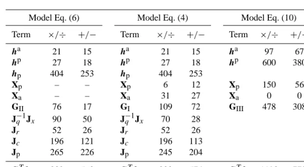
Table 3.Computational effort for solving the inverse dynamic problem.

Model Eq. (6) Model Eq. (4) Model Eq. (10)

Term ×/÷ +/− Term ×/÷ +/− Term ×/÷ +/−

ha 21 15 ha 21 15 ha 97 67

hp 27 18 hp 27 18 hp 600 380

hp 404 253 hp 404 253

Xp – – Xp 6 12 Xp 150 56

Xa – – Xa 31 27 Xa 0 0

GII 76 17 GI 109 72 GIII 478 308

J−q1Jx 90 50 J−q1Jx 70 28

Jr 52 26 Jr 52 26

Jc 196 121 Jc 196 113

Jp 265 226 Jp 245 204

GTh 832 568 GTh 833 574 GTh 1193 773

As Table 3 shows, the models in Eqs. (4) and (6), which are based on splitting the platform from the legs, hold fewer number of operation than those of the model considering the platform attached to one of the legs. This fact is due to the inversion of a 6×6 matrix when finding the matrix GIII. On the other hand, by having the platform attached to one leg, the projection of the platform generalised forces onto the ac-tuated joints is cumbersome. The result shows that either us-ing Eqs. (4) or (6) a reduction of about 30 % in the number of multiplication and about 25 % in additions is obtained when comparing to the model given in Eq. 10). These results in-dicate that considering the platform and legs as subsystem can improve speed in the calculation of dynamics for appli-cations such as model-based control, see for example Díaz-Rodríguez et al. (2013).

5 Conclusions

vector-loop closure constraints introduced the relationship between the dynamics of the open kinematic chains and the original closed chains. A Computer Algebraic Software al-lowed to find each term of the dynamic in symbolic form and to compute the computational burden of each model.

The results showed that the approaches based on splitting the manipulator in two sub-systems (platform and legs) re-quire about 30 % in the number of multiplication and about 25 % in additions are obtained when comparing to the model given by Eq. (10). These results indicate that in problems when the model is needed to be computed on-line at high rates of speed, method 1 and 2 can be useful. This work has provided numerical guidelines for implementing com-putationally efficient models for use in numerically inten-sive optimal mechanical synthesis problems or in resource-constraint embedded computers, particularly for control and model identification. The software support presented for solving the inverse dynamic problem efficiently also provides some insight on some of the advantages and/or disadvantages on these revisited methods.

Acknowledgements. The authors acknowledge the financial support from the Natural Science and Engineering Research council of Canada (NSERC), the New Brunswick Innovation Foundation (NBIF), Fondo Nacional de Ciencia, Tecnología e Innovación (FONACIT-Venezuela), CONACYT scholarship 326912/381134 and also the SNI-México.

Disclaimer. Conflict of interests – the authors declare that the research was conducted in the absence of any commercial, finan-cial, or personal relationships that could be construed as a potential conflict of interests.

Edited by: D. Pisla

Reviewed by: two anonymous referees

References

Angeles, J.: Fundamentals of Robotic Mechanical Systems, Chap-ter 4, 2nd Edn., Springer, 2002.

Carbonari, L., Battistelli, M., Callegari, M., and Palpacelli, M.-C.: Dynamic modelling of a 3-CPU parallel robot via screw theory, Mech. Sci., 4, 185–197, doi:10.5194/ms-4-185-2013, 2013. Carretero, J. A., Nahon, M. A., and Podhorodeski, R. P.: Workspace

analysis and optimization of a novel 3-DOF parallel manipulator, Int. J. Robot. Autom., 14, 178–188, 2000a.

Carretero, J. A., Podhodeski, R. P., Nahon, M. A., and Gosselin, C. M.: Kinematic analysis and optimization of a new three degree-of-freedom spatial parallel manipulator, J. Mech. Design, 122, 17–24, 2000b.

Chapra, S. C. and Canale, R.: Numerical Methods for Engineers, 5th Edn., McGraw-Hill, Inc., New York, NY, USA, 2006. Craig, J. J.: Introduction to Robotics: Mechanics and Control, 3rd

Edn., Pearson Education, Upper Saddle River, NJ, USA, 2005. Díaz-Rodríguez, M., Valera, A., Mata, V., and Valles, M.:

Model-Based Control of a 3-DOF Parallel Robot Model-Based on Identified

Relevant Parameters, IEEE-ASME T. Mech., 18, 1737–1744, 2013.

Fan, K. C., Wang, H., and Chang, T. H.: Sensitivity analysis of the 3-PRS parallel kinematic spindle platform of a serial-parallel ma-chine tool, Int. J. Mach. Tool. Manu., 43, 1561–1569, 2003. Goodwin, G. C., Middleton, R. H., and Poor, H. V.: High-speed

digital signal processing and control, Proceedings of the IEEE, 80, 240–259, 1992.

Ibrahim, O. and Khalil, W.: Kinematic and Dynamic Modeling of the 3-PRS Parallel Manipulator, in: Proceedings of the 12th IFToMM World congress, France, 18–21 June 20017, 1–6, 2007. Khalil, W. and Ibrahim, O.: General Solution for the Dynamic Mod-eling of Parallel Robots, J. Intell. Robot. Syst., 49, 19–37, 2007. Li, Y. M. and Xu, Q. S.: Kinematics and inverse dynamics analysis for a general 3-PRS spatial parallel manipulator, Robotica, 22, 219–229, 2004.

Li, Y. M. and Xu, Q. S.: Kinematic analysis of a 3-PRS parallel manipulator, Robot. CIM. Int. Manuf., 23, 395–408, 2007. Liu, X. J. and Bonev, I. A.: Orientation Capability, Error Analysis,

and Dimensional Optimization of Two Articulated Tool Heads With Parallel Kinematics, J. Manuf. Sci. Eng., 130, 1–9, 2008. Mata, V., Provenzano, S., Valero, F., and Cuadrado, J. I.:

Serial-robot dynamics algorithms for moderately large numbers of joints, Mech. Mach. Theory, 37, 739–755, 2002.

Mata, V., Farhat, N., Díaz-Rodríguez, M., Valera, A., and Page, A.: Dynamic parameters identification for parallel manipulator, Tech Education and Publishing, Vienna, Austria, 21–44, 2008. Merlet, J. P.: Micro parallel robot MIPS for medical applications,

in: Proceedings of the 8th international conference on emerging technologies and factory automation (ETFA 2001), France, 15– 18 October 2001, 611–619, 2001.

Murray, J. and Lovell, G.: Dynamic modeling of closed-chain robotic manipulators and implications for trajectory control, IEEE T. Robotic. Autom., 5, 522–528, 1989.

Parsa, S. S., Carretero, J. A., and Boudreau, R.: Internal redun-dancy: an approach to improve the dynamic parameters around sharp corners, Mech. Sci., 4, 233–242, doi:10.5194/ms-4-233-2013, 2013.

Staicu, S.: Matrix modeling of inverse dynamics of spatial and pla-nar parallel robots, Multibody Syst. Dyn., 27, 239–265, 2012. Tsai, M. S. and Yuan, W. H.: Inverse dynamics analysis for a

3-PRS parallel mechanism based on a special decomposition of the reaction forces, Mech. Mach. Theory, 45, 1491–1508, 2010. Tsai, M. S., Shiau, T. N., Tsai, Y. J., and Chang, T. H.: Direct

kine-matic analysis of a 3-PRS parallel manipulator, Mech. Mach. Theory, 38, 71–83, 2002.

Williamson, D.: Digital Control and Implementation: Finite Wordlength considerations, Prentice Hall, 1991.

Yiu, Y., Cheng, H., Xiong, Z. H., Liu, G., and Li, Z.: On the dynam-ics of parallel manipulators, in: Robotdynam-ics and Automation, 2001, Proceedings 2001 ICRA, IEEE International Conference on, 4, 3766–3771, 2001.