ISSN: 2231-5381
http://www.ijettjournal.org
Page 96
Face Recognition using LBP Coefficient Vectors
with SVM Classifier
Sapna Vishwakarma Prof. Krishan Kant Pathak
M.TECH*(EC) Asst. Professor
TIT Bhopal TIT Bhopal
Madhya Pradesh Madhya Pradesh
Abstract
-
The development of automatic visual control system is a very important research topic in computer vision. In many application including texture based, face recognition system, in this paper we analysis for the face recognition is based on. (1) Local binary pattern is the most successful for face recognition (2) local configuration pattern. Svm technology has been used for face recognition in our work.
Keywords
-
Face Recognition, Support Vector Machine (SVM),Local Binary Pattern (LBP)
1.
Introduction
Continuously increasing security demand is forcing the scientists and researchers to develop robust and advanced security system. Although presently many type of systems are in progress one of them is biometric security which has already proven its effectiveness and considered as most secured and applicable system. This system is particularly preferred or adapted because of its proven natural uniqueness and eliminates the need of carrying additional devices like cards, remote etc.
The biometric security systems refer to the identification of humans by their characteristics .presently the biometric systems are largely used for identification and access control. There are many human characteristics which can be used for biometric identification such that finger print, palm and face etc.amongst them the face is relatively advantageous because of it can be detected from much more distance without need of special sensors or scanning devices this provides easy observation and capability to identify individual in group of persons
There are many face recognition algorithm proposed to improve the efficiency of the system. However, the task of face recognition still remains a challenging problem because of its fundamental difficulties regarding various factor as illumination changes, face rotation, facial expression. The automatic personal recognition system is the most important role. In this paper we use the svm for face recognition system The rest of the paper is arrange as the second section presents a short review of the work done so far, the third section presents the details of technical terms used in the proposed algorithm followed by analysis an conclusion in next chapters.
2. Related Work
ISSN: 2231-5381
http://www.ijettjournal.org
Page 97
first locate facial components, extract them and combine them into a single feature vector which is classified by a Support Vector Machine (SVM).
3. LBP Estimation
Local binary patterns (LBP) are a type of feature used for classification in computer vision. LBP is the particular case of the Texture Spectrum model proposed in 1990. LBP was first described in 1994. It has since been found to be a powerful feature for texture classification. LBPs are usually extracted in a circularly symmetric neighbourhood by comparing each image pixel with its neighbourhood
.
Figure 1: LBP Calculation for three different neighbors.
The LBP feature vector, in its simplest form, is created in the following
Divide the examined window into cells (e.g. 16x16 pixels for each cell).
For each pixel in a cell, compare the pixel to each of its 8 neighbors (on its left-top, left-middle, left-bottom, right-top, etc.). Follow the pixels along a circle, i.e. clockwise or counter-clockwise.
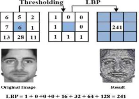
Where the center pixel's value is greater than the neighbor's value, write "1". Otherwise, write "0". This gives an 8-digit binary number (which is usually converted to decimal for convenience).
Compute the histogram, over the cell, of the frequency of each "number" occurring (i.e., each combination of which pixels are smaller and which are greater than the center).
Figure 2: Calculating of LBP
4. Support Vector Machine
(SVM)
Support Vector Machines (SVMs) have developed from Statistical Learning Theory [6]. They have been widely applied to fields such as character, handwriting digit and text recognition, and more recently to satellite image classification. SVMs, like ASVM and other nonparametric classifiers have a reputation for being robust. SVMs function by nonlinearly projecting the training data in the input space to a feature space of higher dimension by use of a kernel function. This results in a linearly separable dataset that can be separated by a linear classifier. This process enables the classification of datasets which are usually nonlinearly separable in the input space. The functions used to project the data from input space to feature space are called kernels (or kernel machines), examples of which include polynomial, Gaussian (more commonly referred to as radial basis functions) and quadratic functions. By their nature SVMs are intrinsically binary classifiers however there are strategies by which they can be adapted to multiclass tasks. But in our case we not need multiclass classification.
4.1 SVM CLASSIFICATION
Let xi∈Rmbe a feature vector or a set of input variables and let yi∈ {+1, −1} be a corresponding class label, where m is the dimension of the feature vector. In linearly separable cases a separating hyper-plane satisfies [8].
Figure 3: Maximum-margin hyper-plane and margins for an SVM trained with samples from two classes. Samples on the
margin are called the support vectors.
Where the hyper-plane is denoted by a vector of weights wand a bias term b. The optimal separating hyper-plane, when classes have equal loss-functions, maximizes the margin between the hyper-plane and the closest samples of classes. The margin is given by
ISSN: 2231-5381
http://www.ijettjournal.org
Page 98
and requires that the partial derivatives of wand bbe zero. In (3), αiis nonnegative Lagrange multipliers. Partial derivatives propagate to constraints . Substituting winto (3) gives the dual form
which is not anymore an explicit function of w or b. The optimal hyper-plane can be found by maximizing (4) subject to
and all Lagrange multipliers are nonnegative. However, in most real world situations classes are not linearly separable and it is not possible to find a linear hyper plane that would satisfy (1) for all i = 1. . . n. In these cases a classification problem can be made linearly separable by using a nonlinear mapping into the feature space where classes are linearly separable. The condition for perfect classification can now be written as
Where Φ is the mapping into the feature space. Note that the feature mapping may change the dimension of the feature vector. The problem now is how to find a suitable mapping Φ to the space where classes are linearly separable. It turns out that it is not required to know the mapping explicitly as can be seen by writing (5) in the dual form
and replacing the inner product in (6) with a suitable kernel function
. This form arises from the same
procedure as was done in the linearly separable case that is, writing the Lagrangian of (6), solving partial derivatives, and substituting them back into the Lagrangian. Using a kernel trick, we can remove the explicit calculation of the mapping Φ and need to only solve the Lagrangian (5) in dual form, where the iSVMer product has been transposed with the kernel function in nonlinearly separable cases. In the solution of the Lagrangian, all data points with nonzero (and nonnegative) Lagrange multipliers are called support vectors (SV).
Often the hyper plane that separates the training data perfectly would be very complex and would not generalize well to external data since data generally includes some noise and outliers. Therefore, we should allow some violation in (1) and (6). This is done with the nonnegative slack variable ζi
The slack variable is adjusted by the regularization constant C, which determines the tradeoffs between complexity and the generalization properties of the classifier. This limits the Lagrange multipliers in the dual objective function (5) to the range 0 ≤ αi ≤ C. Any function that
is derived from mappings to the feature space satisfies the conditions for the kernel function.
The choice of a Kernel depends on the problem at hand because it depends on what we are trying to model The SVM gives the following advantages over neural networks or other AI methods (link for more details http://www.svms.org).
SVM training always finds a global minimum, and their simple geometric interpretation provides fertile ground for further investigation.
Most often Gaussian kernels are used, when the resulted SVM corresponds to an RBF network with Gaussian radial basis functions. As the SVM approach “automatically” solves the network complexity problem, the size of the hidden layer is obtained as the result of the QP procedure. Hidden neurons and support vectors correspond to each other, so the centre problems of the RBF network is also solved, as the support vectors serve as the basis function centres.
Classical learning systems like neural networks suffer from their theoretical weakness, e.g. back-propagation usually converges only to locally optimal solutions. Here SVMs can provide a significant improvement.
The absence of local minima from the above algorithms marks a major departure from traditional systems such as neural networks.
SVMs have been developed in the reverse order to the development of neural networks (SVMs). SVMs evolved from the sound theory to the implementation and experiments, while the SVMs followed more heuristic path, from applications and extensive experimentation to the theory.
5. Proposed Algorithm
The proposed algorithm can be described in following steps.
1. Firstly divide the image into NxN blocks
2. Take the LBP of the image depending upon the technique to be used.
3. Now select any of the variants from uniform, rotation invariant and uniform rotation invariant depending upon the variants to be used.
4. Like above step these vectors are created for all classes of faces.
5. SVM classifiers are used one against one method.
6. For detection purpose the input image vectors are calculated in same way as during training and then it is applied on each
classifier.
6.
Simulation Results
ISSN: 2231-5381
http://www.ijettjournal.org
Page 99
The accuracy of the algorithm is tested for different number of faces, samples and vector length.
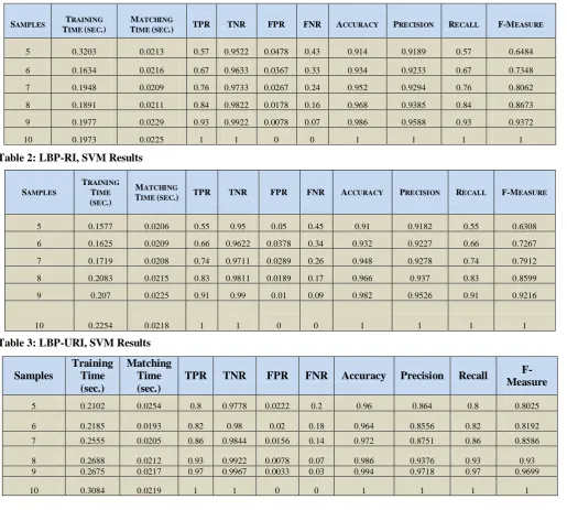
Table 1: LBP-U, SVM Results
The comparison of the different variants of LBP with SVM. For all test results the total 10 faces with 10 samples each are used although the training samples are from 5 to 10.
Table 2: LBP-RI, SVM Results
Table 3: LBP-URI, SVM Results
7.
CONCLUSION
This paper presents a LBP approaches for feature extraction and during the classification phase, the Support Vector Machine (SVM) is tested for robust decision in the presence of wide facial variations. . In this paper we have developed, tested and compared all three variants of LBP in future we can also compare them with using different kernel functions and learning techniques
8. REFERENCES
[1] YimoGuo, Guoying Zhao , MattiPietikainen and Zhengguang Xu”Descriptor Learning Based on Fisher Separation Criterion for Texture Classification”, Computer Vision – ACCV 2010 Lecture Notes in Computer Science Volume 6494, 2011, pp 185-198.
[2] IgnasKukenys and Brendan McCane “Support Vector Machines for Human Face Detection”, NZCSRSC ’08 Christchurch New Zealand
SAMPLES TRAINING
TIME (SEC.)
MATCHING
TIME (SEC.) TPR TNR FPR FNR ACCURACY PRECISION RECALL F-MEASURE
5 0.3203 0.0213 0.57 0.9522 0.0478 0.43 0.914 0.9189 0.57 0.6484
6 0.1634 0.0216 0.67 0.9633 0.0367 0.33 0.934 0.9233 0.67 0.7348
7 0.1948 0.0209 0.76 0.9733 0.0267 0.24 0.952 0.9294 0.76 0.8062
8 0.1891 0.0211 0.84 0.9822 0.0178 0.16 0.968 0.9385 0.84 0.8673
9 0.1977 0.0229 0.93 0.9922 0.0078 0.07 0.986 0.9588 0.93 0.9372
10 0.1973 0.0225 1 1 0 0 1 1 1 1
SAMPLES
TRAINING
TIME
(SEC.)
MATCHING
TIME (SEC.) TPR TNR FPR FNR ACCURACY PRECISION RECALL F-MEASURE
5 0.1577 0.0206 0.55 0.95 0.05 0.45 0.91 0.9182 0.55 0.6308
6 0.1625 0.0209 0.66 0.9622 0.0378 0.34 0.932 0.9227 0.66 0.7267
7 0.1719 0.0208 0.74 0.9711 0.0289 0.26 0.948 0.9278 0.74 0.7912
8 0.2083 0.0215 0.83 0.9811 0.0189 0.17 0.966 0.937 0.83 0.8599
9 0.207 0.0225 0.91 0.99 0.01 0.09 0.982 0.9526 0.91 0.9216
10 0.2254 0.0218 1 1 0 0 1 1 1 1
Samples
Training
Time
(sec.)
Matching
Time
(sec.)
TPR
TNR
FPR
FNR
Accuracy
Precision
Recall
F-Measure
5 0.2102 0.0254 0.8 0.9778 0.0222 0.2 0.96 0.864 0.8 0.8025
6 0.2185 0.0193 0.82 0.98 0.02 0.18 0.964 0.8556 0.82 0.8192
7 0.2555 0.0205 0.86 0.9844 0.0156 0.14 0.972 0.8751 0.86 0.8586
8 0.2688 0.0212 0.93 0.9922 0.0078 0.07 0.986 0.9376 0.93 0.93
9 0.2675 0.0217 0.97 0.9967 0.0033 0.03 0.994 0.9718 0.97 0.9699
ISSN: 2231-5381
http://www.ijettjournal.org
Page 100
[3] YimoGuo, GuoyingZhao ,MattiPietikainen”Texture Classification using a Linear Configuration Model based Descriptor”,BMVC 2011 http://dx.doi.org/10.5244/C.25.119.
[4] TimoOjala, MattiPietikäinen and TopiMäenpaa “A Generalized Local Binary Pattern Operator for Multiresolution Gray Scale and Rotation Invariant Texture Classification”,Pattern Analysis and Machine Intelligence, IEEE Transactions (Volume:24 , Issue: 7 ), Jul 2002.
[5] Jennifer Huang, Volker Blanz and Bernd Heisele “FaceRecognition Using Component-Based SVM Classification and Morphable Models”, SVM 2002, LNCS 2388, pp. 334–341, 2002. Springer-Verlag Berlin Heidelberg 2002.
[6] Guoying Zhao and MattiPietikainen”Dynamic Texture Recognition Using Local Binary Patterns with an Application to Facial Expressions”,IEEE TRANSACTIONS ON PATTERN ANALYSIS AND MACHINE INTELLIGENCE, 2007.
[7] TimoAhonen, Jirı Matas, Chu He, and MattiPietikainen “Rotation Invariant Image Description with Local Binary Pattern Histogram Fourier Features”,Image Analysis Lecture Notes in Computer Science Volume 5575, 2009, pp 61-70.