http://www.sciencepublishinggroup.com/j/ajam doi: 10.11648/j.ajam.20170504.11
ISSN: 2330-0043 (Print); ISSN: 2330-006X (Online)
Mathematical Modeling and Simulation Study for the
Control and Transmission Dynamics of Measles
Selam Nigusie Mitku, Purnachandra Rao Koya
*School of Mathematical and Statistical Sciences, Hawassa University, Hawassa, Ethiopia
Email address:
[email protected] (S. N. Mitku), [email protected] (P. R. Koya) *Corresponding author
To cite this article:
Selam Nigusie Mitku, Purnachandra Rao Koya. Mathematical Modeling and Simulation Study for the Control and Transmission Dynamics of Measles. American Journal of Applied Mathematics. Vol. 5, No. 4, 2017, pp. 99-107. doi: 10.11648/j.ajam.20170504.11
Received: April 15, 2017; Accepted: May 2, 2017; Published: July 6, 2017
Abstract:
In this paper, a five compartmental model has been considered and investigated the transmission dynamics of measles disease in the human populations. The only one infected compartment in the standard model has been split into two: Infected catarrh, and infected eruption. Measles is a deadly disease that is very common and contagious in the world. However, if enough care is taken one can survive easily against Measles disease. The Measles disease has no specific treatment but vaccination is available. It has been shown that the model has a positive solution and is bounded. The basic reproduction number is derived using the next generation matrix method. The disease free equilibrium point is found and endemic equilibrium state is identified. It is shown that the disease free equilibrium point is locally and globally asymptotically stable if the reproduction number takes a value less than one unit and unstable if it is more than one unit. Numerical simulation study is conducted using ode 45 of MATLAB. The results and interpretations are elaborated and included in the text. Description of the model, Mathematical analysis, stability analysis, and simulation studies are conducted and the results are included. The standard model and the proposed models have been compared and the observations are presented in a tabular form.Keywords:
Measles, Modeling, Equilibrium Points, Stability Analysis, Reproduction Number, Simulation Study1. Introduction
Measles is one of the communicable diseases still causing preventable mortality and morbidity in the country. It is also one of the most contagious but vaccine preventable diseases which is caused by the paramyxovirus family from the morbilli virus genus. Even thought an effective vaccine is available and widely used measles continuous to occur even in developed countries. It is a child hood disease that rarely occurs in adults. Measles is respiratory disease caused by virus. Paramyxovirus is normally growth in the cells that line the back of the throat and lungs. Measles is an infectious diseases highly contagious through person-to-person transmission mode, with more than 90% secondary attack rates among susceptible persons. It resides in the mucus in the nose and throat of an infected person, so transmission typically occurs through coughing and sneezing [1 – 3].
Measles is a disease of all climates and races, and susceptibility is universal. It must have been common in the
ancient world, but no accurate account occurs in history until the classical description by Rhazes in AD. Sever measles are more likely among poorly nourished young children, especially those with insufficient vitamin A or who immune systems have been weakened by HIV/AIDS or other diseases. Measles is a disease of humans; measles virus is not spread by any other animal species. Measles is both an epidemic and endemic disease, it is difficult to accurate estimate its incidence on the global level, particularly in the absence of reliable surveillance systems. Although many counties reported the number of incidence cases directly to
WHO, the heterogeneity of these systems with differential under reporting under reporting does not permit an accurate assessment of the global measles incidence [4 – 5].
Pathogenesis: Measles is a systemic infection. The primary site of infection is the respiratory epithelium of the nasopharynx. Two to three days after invasion and replication in the respiratory epithelium and regional lymph nodes, a primary viremia occurs with subsequent infection of the reticuloendothelial system. Following further viral replication in regional and distal reticuloendothelial sites, there is a second viremia, which occurs 5 to 7 days after infection. During this viremia, there may be infection of the respiratory tract and other organs. Measles virus is shed from the nasopharynx beginning with the prodromal until 3 to 4 days after rash onset.
Symptoms and signs of Measles: Prodromal or catarrh, and general symptoms of measles infection presents with a two to four day prodromal of fever, malaise, cough, and runny nose or coryza prior to rash onset. Conjunctivitis and bronchitis are commonly present. Although there is no rash at disease onset, the patient is shedding virus and is highly contagious. A harsh, non-productive cough is present throughout the febrile period, persists for one to two weeks in uncomplicated cases, and is often the last symptom to disappear. Generalized lymphadenopathy commonly occurs in young children. Older children may complain of photophobia and, occasionally, of arthralgia. Measles confer lifelong immunity from further attacks [3].
Catarrh or Prodromal Stage: A fever of about 38 degree centigrade and catarrhal symptoms such as nasal discharge, sneezing, eye discharge and cough persist for three to four days. The respiratory secretions, lacrimal fluid and saliva at this stage are at their most infectious. On the last one to two days of the catarrhal symptoms, punctate white macules called Koplik's spots appear on the buccal mucosa.
Eruption Stage: After the fever subsides, it recurs biphasic fever, accompanied by eruptions and aggravation of the catarrhal symptoms. It persists for three or four days. Eruptions first appear behind the ears and cheeks, spreading to the trunk and extremities. Small erythematic coalesces and enlarges, forming irregular shapes with a reticular pattern. By this time Koplik's spots have already disappeared. The measles virus is not found at the lesion; the mechanism is thought to be allergic reaction. Dehydration and various complications often occur from the persistent high fever.
Recovery Stage: The fever subsides in several days. Healing is with exfoliation of eruptions and pigmentation.
Treatment: The treatment of measles embraces the preventive measure to be adopted in the cause of an outbreak by the isolation of the sick at as early a period as possible. Epidemics have often specially in limited localities, been curtailed by such a precaution. There is no specific treatment for measles. People with measles need bed rest, fluids, and control of fever. Patients with complications may need treatment specific to their problem. Measles vaccination is one of the most cost-effective interventions available.
Here some important terminology that is frequently used in this work is now introduced. Compartmentalize a group of persons with similar status or with respect to the same disease. A person is said to be susceptible if that has not yet
infected by the disease but likely to get the disease in future. A person is said to be exposed to a disease when the virus enters into the person's body. At this stage the effects of the disease cannot be identified with the person, because the effects are in sleeping state. A person is said to be infected if it has the disease in its body and is able to transfer the disease to other susceptible persons [8 – 10].
Incubation period is approximately ten to twelve days from exposure to the onset of fever and other nonspecific symptoms and fourteen days, with a range of seven to eighteen days, from exposure to the onset of rash. Measles can be transmitted from four days before rash onset i.e., one to two days before fever onset, to four days after rash onset. Infectivity is greatest three days before rash onset. Measles is highly contagious. Secondary attack rates among susceptible household contacts have been reported to be 75% to 90%. Due to the high transmission efficiency of measles, outbreaks have been reported in populations where only 3% to 7% of the individuals were susceptible. Whereas vaccination can result in respiratory excretion of the attenuated measles virus, person-to-person transmission has never been shown [11 – 12].
The mathematical modeling of infectious diseases is used to study the means by which diseases spread, to forecast the future course of an outbreak and to evaluate strategies to control an epidemic. Momoh and many researchers developed a mathematical model for control of measles epidemiology. They used model to determine the impact of exposed individuals at latent period through the stability analysis and numerical simulation. But here in the present study, the infectious compartment is replaced with (i) Catarrh and (ii) Eruption compartments. Thus, the modified model is named as and is used in the present work for further analysis and interpretations [13 – 14].
2. Modeling and Formulations of
Measles Disease
Here now and SEI I R models are formulated for describing the dynamics of Measles. The whole person population is categorized into susceptible, exposed, infected and removed groups for model and susceptible, exposed, infected but in Catarrh or prodromal stage ; infected but Eruption stage , recover groups for model. Susceptible or Individuals who may get the disease, Exposed or Latent or Individuals who are exposed to the disease, Infectious or Individuals who have the disease and are able to transfer it to others, Recovered or Individuals who have permanent infection-acquired immunity.
2.1. Mathematical Modeling Using Compartments
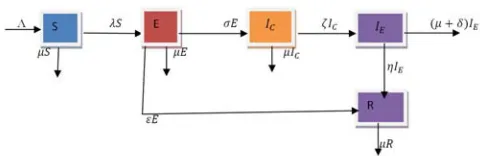
Figure 1. Compartmental diagram of the model.
The mathematical equations describing the model can be described by a system of ordinary differential equations as:
dS dt⁄ βS I N⁄ (1)
dE dt⁄ βS I N⁄ (2)
dI dt⁄ (3)
dR dt⁄ (4)
HeredN dt⁄ 0 and . In the compartment model the population is assumed to be closed. That is, births, deaths and migrations are considered to be negligible and omitted. Thus, the population size parameter is a constant. Here represents the number of individuals those are susceptible to the disease but not infected at time. The parameter denotes the number of individuals those are exposed to the virus or infected but not yet tested positive of the infection. The parameter denotes the number of infected individuals who are able to spread the disease to other susceptible people, and represents the number of individuals those have successfully gained immunity from the disease die or removed by death. After exposed by the virus the individuals from the susceptible compartment enters the exposed compartment before they become infectious individuals and later either recover or die. The parameter represents the transmission rate of disease from susceptible to exposed, is rate at which an infected individual becomes infectious per unit time. Similarly, 1⁄ and 1⁄ are the average durations of incubation and infectiousness periods respectively. 2.2. Assumptions of the Model In this study , Susceptible, Exposed, Infected, Recovered, epidemic model have been considered and classified the infected population I as those first stage or catarrh I and second stage or eruption I . A simulation study will also be conducted by assigning different valid values to the parameters of the model. The present model has a compartmental structure and is designed based on the assumptions described as follows: a. Assume that the susceptible people are recruited from the total population at a constant rateΛ. b.The population is homogeneously mixing and reflects increasing dynamics. c. The class is decreased by testing and measles therapy at a rate !. d.There is adequate contact of a susceptible individual with an Infective individual then transmission may occur, thus the susceptible individuals may join the exposed class at a rate "#β c I I % N⁄ &. e. When latent period ends, exposed individuals may progress to the infected catarrh class I , at rate . f. The way the individual can leave from the infected catarrh class to infected eruption class I with the rate '. g.After some treatment, infected eruption individuals may recover and join the recovery class R, at rate η . h.The disease is fatal, infected eruption individuals may die due to the disease at the rate ) or die naturally at rateµ. i. Also assume that both recovered exposed individuals and recovered infected eruption individuals become permanently immune to the disease. Basically the present model is a new model and is a model. 2.3. Description of Variables and Parameters The following tables describe the variables and parameters used in this model: Table 1. Description of Variables used in the model equations (5) to (9). Variable * Description The total population at time t The number of Susceptible individuals at time t E The number of Exposed individuals at time t The number of Infected catarrh individuals at time t The number of Infected eruption individuals at time t R The number of Recovered individuals at time t Table 2. Description of parameters used in the model equations (5) to (9). Parameter Description Λ birth or immigration rate Force of infection, + / Progression rate from latent to infectious ' Progression rate from infected catarrh to infected eruption ! testing and measles therapy rate - Recovery rate of treated infectious individuals ) Death due to disease Probability of one infected individual to become infectious + Per Capita contact rate . Natural death rate unrelated to the disease The flow diagram of model is given in Figure 2 Figure 2. Control and Transmission Dynamics of Measles. The mathematical formulation of model can be expressed as systems of differential equation as follows: / /⁄ Λ . (5)
dE dt⁄ λ S σ ε μ E (6)
dI dt⁄ = ζI − (η + δ + μ)I (8)
/ /⁄ = - + ! − . (9) Here = "# +( + ) %⁄ &. The total population size
is = + + + + .
2.4. Positivity of the Solutions
Here now it is to be shown that all state variables remain non-negative since they represent human population. Π =
"( , , , , ) ∈ ℜ:; (0) > 0, (0) > 0,
(0) >
0, (0) > 0, (0) > 0&. It is to be shown that the solutions of, " ( ), ( ), ( ), ( ), ( )& from the system of equations (5) – (9), are all non-negative for all ≥ 0.
The equation / /⁄ = Λ − ( + .) , without loss of generality, can be expressed as / /⁄ ≥ −( + .) . The algebraic solution of this inequality is obtained as ( ) ≥
S(0)>?(@AB)C. Further in the limit as → ∞ it is observed
that S( ) → S(0) . Thus, the size of the susceptible population is always non–negative i.e. S(t) ≥ 0.
The equation / /⁄ = − ( + ! + .) , without loss of generality, can be expressed as / /⁄ ≥ −( + ! + .). The algebraic solution of this inequality is obtained as ( ) ≥ E(0)>?(FAGAB)C. Further in the limit as → ∞ it
can be observed that ( ) → E(0). Thus, the size of the
exposed population is always non – negative i.e. ( ) ≥ 0. The equation/ /⁄ = − (' + .) , without loss of generality can be expressed as / /⁄ ≥ −(' + .) . The algebraic solution of this inequality is obtained as ( ) ≥
I (0)>?(HAB)C. Further in the limit as → ∞ it can be
observed that ( ) → (0).Thus, the size of the infected catarrh population is always non – negative i.e. ( ) ≥ 0.
The equation / /⁄ = ' − (- + ) + .) , without loss of generality can be expressed as / /⁄ ≥ −(- + ) +
.) . The algebraic solution of this inequality is obtained as ( ) ≥ I (0)>?(IAJAB)C. Further in the limit as →
∞ it can be observed that ( ) → I (0). Thus, the size of the infected eruption population is always non-negative i.e. ( ) ≥ 0.
The equation/ /⁄ = - + ! − . , without loss of generality can be expressed as / /⁄ ≥ −. . The algebraic solution of this inequality is obtained as ( ) ≥ R(0)>?BC. Further in the limit as → ∞ it can be observed that ( ) →
(0). Thus, the size of the recovered population is always non – negative i.e. ( ) ≥ 0.
2.5. Invariant Region
Since the model (2) monitors human populations, all the associated parameters and state variables are non-negative for all ≥ 0. It is easy and straight forward to show that the state variables of the model remain negative for all non-negative initial conditions. Consider the biologically feasible region Π = " , , , , & ∈ ℜ: such that → (Λ .⁄ ).
Lemma 1: The closed region Π is positively invariant and attracting.
Proof: Adding equations (5) through (9) gives the rate of change of the total population / /⁄ = Λ − . . Thus, the total human population is bounded by Λ .⁄ , so that
dN dt⁄ = 0, whenever ( ) = Λ .⁄ . It can be shown that ( ) = Λ .⁄ + # L− ( Λ .⁄ )% >?BC . In particular as
→∞
( ) = Λ .⁄ (10) Hence the region Π is positively invariant and attracts all solution in ℜ5.
3. Stability Analysis of the Model
This section is mainly aimed to (i) identify the existence of equilibrium points viz. disease free equilibrium point, endemic equilibrium point (ii) analyze local stability of disease free equilibrium point and endemic equilibrium point and (iii) construct the formula for reproduction number.
3.1. Existence of Equilibrium Points
The equilibrium points are obtained by setting the right hand sides of the system of model equation (2) to zero. That means/ /⁄ = / /⁄ = / /⁄ = / /⁄ = / /⁄ =0.
The fore going set of conditions is a requirement for existence of equilibrium points.
3.2. Disease Free Equilibrium
Disease free equilibrium point denoted by 0 is a steady
state solution. At this point there will be no measles disease. The human populations of exposed, infected – catarrh and infected – eruption compartments can be considered as measles infected.
Let 0= M 0∗, 0∗, 0
∗,
0
∗,
0∗O represents the
disease free equilibrium point of the model equation (2). Hence, in the absence of infection it takes = = =
=0 and the equilibrium points are obtained by setting the
right hand sides of the model equations (6) – (9) to zero. Then the co-ordinates of the disease free equilibrium point
0 will be obtained as
0= ( 0∗, 0, 0, 0, 0 ) (11)
Here in (11) the notation used is 0∗= Λ .⁄ .
3.3. Basic Reproduction Number
In order to assess the local stability of the disease free equilibrium point 0 which is to be established by the next
generation method on the system (2), computation of the basic reproduction number is essential. The basic reproduction number 0 is a threshold parameter defined as
the average number of secondary infections caused by an infectious individual when introduced into a completely susceptible population. It is also called basic reproduction ratio or basic reproductive rate [10].
If more than one secondary infection is produced from one primary infection that is 0> 1, then an epidemic occurs.
When 0< 1 then there is no epidemic and it means that
the disease dies out over a period of time. When 0= 1
remains in the population at a constant rate as one infected individual transmits the disease to one susceptible individual only in [8].
In the model of the present study three of five compartments are with infected populations. They are , and . Let, QR , S = 1, 2, … , V be the numbers of infected individuals in S CW the infected compartment at time . Let the variable Q be defined as a vector of the populations of all in infected compartments i.e. Q = # QX QY … QZ%. Let
[R(Q) be the rates of appearance of new infections in the
corresponding infected compartments. Let \R(Q) be the difference between rates of transfer of individuals for the
S CW compartment.
Similarly, \RA(Q) be the rate of transfer of individuals into
S CW compartment by all other means. Also \
R?(Q), be the
rate of transfer of individuals out of S CW compartment by all other means.
Now the rate of change of population size in the
S CW infected compartment can be obtained as /Q
R⁄ =/
[R(Q) − \R(Q), where \R(Q) = \RA(Q) − \R?(Q). Thus, the equation can also be expressed equivalently as /QR⁄ =/
[(Q) − \(Q). Here the notations used to represent the
column vectors
are [(Q) = #[X(Q), [Y(Q), … , [Z(Q)%] and \(Q) =
#\X(Q), \Y(Q), … , \Z(Q)%].
Now the basic reproduction number is computed using the next generation matrix approach by taking the infected compartments , and . The rates of changes of populations of these compartments are given by the equations, respectively, (6) to (8).
First the matrices ^R and \R are constructed and then the corresponding matrices of partial derivatives [ and \. Also the inverse matrix \?X is to be found. Finally the reproduction number L will be computed as the trace of the matrix product [\?X . By linearization approach, the associated matrix at disease free equilibrium is obtained as
^R= _
# +( + ) %⁄ 0
0 `, \R= _
( + ! + .) ' + . −
- + . + ) − ' ` (12)
Now let us partially differentiate the variables , and with respect to time and then evaluate them at the disease free equilibrium point. On substituting these and after some algebraic simplifications, the Jacobean matrices take the form as
[ =aQa^R
R= _
0 ( + ∗L⁄ ) ( + ∗L⁄ )
0 0 0
0 0 0 `
\ = _ + ! + .− ' + .0 00
0 −' - + . + )`
\?X=
b c c c
d (FAGAB)X 0 0
F M(FABAG)(HAB)O X (HAB) 0 FH M(FABAG)(HAB)(IAJAB)O H M(IAJAB)(HAB)O X (JAIAB)ef
f f g
(13)
[\?X( L) = _
( +p ijk⁄ ) + l jk⁄ + k⁄
0 0 0
0 0 0 ` (14)
Here in (14), l = (- + ) + . + '), i = ( + . +
!), k = (- + ) + .) and j = ' + ..
Now the eigenvalues m of [\?X( L) the matrix (14) are to be computed. The eigenvalues are found by solving the characteristic equation
|[\?X(
L) − m | = 0 (15)
The characteristic equation (15) takes the simple form as
mo− pmY= 0. Thus, the three eigenvalues are m
X= mY= 0
andmo= p = ( +Λ p ijk⁄ ). But the reproductive number is defined as L= qM[\?X( L)O = max "mX, mY, mo&. Here q is the spectral radius of [\?X at the disease free equilibrium point L. Hence it follows that the basic reproduction number L for the system of model equations (2) with control strategies and transmission has been constructed and is given by
L= "# +(- + ) + . + ')% #( + . + !)(' + .)(- + ) + .)%⁄ & (16)
3.4. Local Stability of the Disease Free Equilibrium Point
The local stability of the disease free equilibrium point is of three types and the corresponding names and conditions can be stated as follows: (1) the disease free equilibrium point L is said to be locally asymptotically stable if the real parts of the eigenvalues are all negative and unstable if the real parts of the eigenvalues are positive. (2) If L< 1 then disease free equilibrium point is locally asymptotically stable i.e. no measles epidemic can develop in the population and (3) if L> 1 then the disease free equilibrium point L is unstable i.e. measles epidemic can develop in the population.
Now, the equilibrium point L= " L∗, L∗, L∗, L∗,
L∗& can be analyzed by computing the Jacobean matrix of
the model equations (5) to (9). Now differentiate each equation of the system to with respect to , , , and and then evaluating the resultants at the disease free equilibrium point, to get
u( L) =
b c c c
d −. 0 + 0 + 0 0 0 0 −( + ! + .) 0 ! + −(' + .) ' 0 + 0 −(- + . + )) -0 0 0 −.ef f f g (17)
Consider the matrix (18) and let v be the eigenvalues of the characteristic equation
|u( L) − v | = 0 (18)
As the first and fifth columns in (18) correspond to the total human populations and contain only the diagonal terms, these diagonal terms form two similar eigenvalues of the Jacobean matrix. Thus, setting #−(. + v)% = 0 implies that
vX= v: = −. < 0.This is in accordance with condition 1 stating that Lis stable.
characteristic equation of the matrix formed by excluding the first and fifth rows and first and fifth columns of (18), the resultant equation is obtained as
w−( + ! + . + v) −(' + . + v)+ 0+
0 ' – (- + . + ) + v)w = 0 (19)
Also, the characteristic equation (19) can be expressed as
vo+ p
LvY+ pXv + pY = 0 (20)
In (20), the notations used are pL= #- + ' + ! + + ) +
3.%, pX= #( + z + .)(- + . + )) + (' + .)(- + . + )) +
(! + + .)(' + .) − +%, pY= #(' + .) (- + ) +
.)( + ! + .) − + (- + ) + . + ')%.
By Routh-Hurwitz criteria the three roots of (20) are real distinct and negatives if pL> 0, pX> 0 and pLpX> pY; those lead to the following condition on the parameters:
"#- + ' + ! + + ) + 3.% #( + z + .)(- + . + )) + (' + .)(- + . + )) + (! + + .)(' + .) − +%& > #(' + .) (- + ) + .)( + ! + .) − + (- + ) + . + ')%(21)
This implies that (1 − L) > 0 or equivalently L< 1. Hence, according Condition 2 the disease free equilibrium point is locally stable. Thus, it can be concluded that the disease free equilibrium point Lis locally stable.
3.5. Global Stability of the Disease Free Equilibrium Point
In this section, the global properties of the disease free equilibrium point are studied. The global property of the disease free equilibrium point is provide in the form of a theorem as stated in the following:
Theorem 1: If the reproduction number satisfies the condition then the disease free equilibrium point L= (Λ .⁄ ,
0, 0, 0, 0)is globally asymptotically stable in the region Π. Further, if L> 1 then L is unstable.
Proof: By the comparison theorem the rate of change of the variables representing the infected components of model system (2) can be rewritten as
{/ // /⁄⁄
/ /⁄ | ≤ #[ − \% _ ` (22)
Here in (22), #[ − \% represents a matrix as
#[ − \% =
{−( + ! + .) +( + ) ⁄ −(' + .) +( + ) ⁄0
0 ' −(- + ) + .) | (23)
It has been seen that the eigenvalues of the matrix #[ − \% given in (23) are located on its main diagonal and are real and negative that is −( + z + .), −(' + .) and −(- +
) + .). It follows that the system of linear differential inequalities (22) is stable whenever L< 1. Also it can be observed that → 0, → 0 p~/ → 0 pm → ∞. Further evaluation of the system of equations (5) − (9) at = =
= = 0 and when L< 1 results in obtaining =
Λ .⁄ . Therefore, the disease free equilibrium point L is globally asymptotically stable in the region Π.
3.6. Endemic Equilibrium Point
Endemic equilibrium point X∗is a steady state solution, where the disease persists in the population. The existence and uniqueness of endemic equilibrium point X∗ should satisfy the conditions: X∗= " ∗( ), ∗( ), ∗( ), ∗( ),
∗( )& and X∗= " ∗( ), ∗( ), ∗( ), ∗( ), ∗( )& >
0. It is now needed to find the endemic equilibrium points of the system (5) – (9). Setting the right hand sides of the system to zero gives
Λ − +( ∗+ ∗) ∗⁄ − . = 0 (24)
+( ∗+ ∗) ∗⁄ – ( + ! + .) ∗= 0 (25) ∗− (' + .) ∗= 0 (26)
' ∗− (- + ) + .) ∗= 0 (27)
- ∗+ ! ∗− . ∗=0 (28)
On solving (24) – (28), the solutions are obtained as
∗= (Λ .⁄ ) (1⁄ )L ∗
= (Λ + ! + .⁄ )
− #Λ(' + .)(- + ) + .) + (- + ) + ' + .)%⁄
∗= # Λσ (' + .)( + ! + .)% #1 − (1 L
⁄ )% ⁄
∗= #Λσ' (' + .)( + ! + .)(- + ) + .)⁄ % #1 − (1 L
⁄ )%
∗= •#FHIAG(HAB)(IAJAB)%
#B(HAB)(FAGAB)(IAJAB)% #1 − (1⁄ )%L
3.7. Local Stability of Endemic Equilibrium Point
Measles is a kind of endemic disease that constantly presents with a greater or lesser degree among the people of certain class or among the people living in a particular location. If L> 1 the the system has an endemic infection because of the introduction of secondary infection. To show local stability of endemic equilibrium points of system (5) – (9), Routh-Hurwitz criteria can be used.
Theorem 2: The positive endemic equilibrium point X∗ of the system of equations (5) – (9) is locally asymptotically stable if L> 1.
Proof: Since L> 1 the parameters ∗, ∗, ∗, ∗ and
∗ all are non negative terms. The Jacobian matrix of the
system at the endemic equilibrium point takes the form
u( X∗) =
b c c c
d−l − .l 0 − + ∗⁄ − + ∗⁄ 0
0 0
−‚ 0
+ ∗⁄
−j
' − + ∗⁄
0
−k 0 0 0 0 ! 0 - − . ef
f f g
(29)
Here in (29), the notations used are including l =
and j = ' + .. Also from equation (10) it can be had that ( ) =Λ⁄.. The characteristic equation |u( X∗
v | 0 of the Jacobean matrix (29) at X∗ takes the form
as
b c c c
d l . vl 0 + ∗⁄ + ∗⁄ 0
0 0
‚ v
0
+ ∗⁄
j v '
+ ∗⁄
0 k v
00 0 0 ! 0 - . vef
f f g
0 (30)
Here in (30), k is the eigenvalues and is the identity matrix of class 5 ƒ 5. The characteristic polynomial of (30) is of the form as
„ v v: …
X†‡ …Yvo …ovY …‡v …: (31)
Here in 31 , the notations used are
…X 2. l k j ‚
…Y 2.‚ l‚ lj lk 2.k 2.j .l .Y j‚
k‚ jk . + ∗⁄Λ
…o l‚j .‚j lk‚ 2.k‚ .l‚ .Y‚ lkj
2.kj .lj .Yj .lk .Yk
kj‚ . +l ∗⁄ Λ
#. + ∗ 2. l k ' Λ⁄ %
…‡ l‚jk 2.‚jk .l‚j .Y‚j .lk‚ .Y‚k
.lk‚ .Ykj . +l ∗# μ v Λ⁄ %
. + ∗# .l .Y 2. k lk Λ⁄ %
'. + ∗ # 2. l Λ⁄ %
…: .ljk‚ .Yjk‚ .Y +k ∗ # .k ' l . ⁄ %Λ.
Due to the complexity in determining the signs of the eigenvalues of (31), now the Routh-Hurwitz conditions for stability are employed. By Routh-Hurwitz criteria the determinant becomes positive if the following conditions hold true …X< 0, …Y< 0, …o< 0, …‡< 0, …:< 0, …o…‡<
…Y…:, …X…Y…:< …o and …:< …X…‡. It is required to assign
values to the parameters so that all these requirements will hold true in our model.
Therefore all the roots of the characterize polynomial of equation 31 are negative. Thus, it can be concluded that the system 2 is locally asymptotically stable.
4. Numerical Simulations
Numerical simulation of the model equations (5) to (9) were carried out using MATLAB inbuilt function ode 45. The main objective of this study is to assess the response of model parameters on the transmission dynamics of the disease. Also investigated the impact of exposed individual at latent period and conducted simulation study. The parameter is considered and assigned different values, few of which are less and the other is greater than one unit, and conduct simulation study.
Since, most of the parametric values are not readily available it is needed to assign some arbitrary values. However, some are available [11 – 12]. Thus, the remaining
is set as follows: and. Further, the initial conditions have been considered as and at initial time. Also the final time is considered as. The results of the simulation study are presented in the following figures:
Figure 3. Population dynamics of five compartment model.
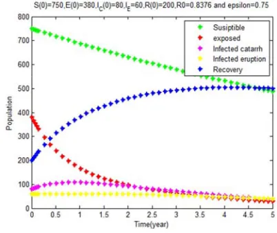
In Figure 3, simulation study shows the result of the impact of testing and therapy of exposed individual at latent period with the rate and the reproduction number and the other parameter value are taken as mentioned above. The population dynamics of epidemic compartmental model is considered. The susceptible and the number of exposed latent individuals decrease steadily. Also the number of infective with early symptom or infected catarrh compartment individuals decrease to zero. The number of infected with later symptom or infected eruption compartment individuals are decreasing. Recover compartment increases steadily and approaches to 412. Finally the epidemic seems dies out.
Figure 4. Population dynamics of five compartment model.
with early symptom or infected catarrh increase initially and then decrease during later times. The infectives with later symptom or infected eruption decrease steadily. Recover compartment increases steadily and approaches 484 during initial times and then starts decreasing to 430 during the later times. Finally the epidemic seems dies out.
Figure 5. Population dynamics of five compartment model.
In figure 5, simulation study shows the result of the impact of testing and therapy of exposed individual at Latent period at the rate and the reproduction number and the other parameter value are as stated above. The population dynamics of epidemic compartmental model is considered. The number of exposed latent individual increases to 384 during initial times and then starts decreases steadily to 190. Also the number of infective with early symptom or infected catarrh compartment individuals increase to 98. The number of infected with later symptom or infected eruption compartment individuals are increasing to 67. Recover compartment increases to 480. Finally the epidemic seems exist. This means that one infected person can transmit disease for more than one person and the spread of measles disease continuous in the society.
Figure 6. Population dynamics of five compartment model.
In figure 6, simulation study shows the result of the impact of testing and therapy of exposed individual at Latent period with the rate and the reproduction number and the other parameter values are as mentioned above. The population dynamics of epidemic compartmental model are considered. The exposed latent individuals increase to 382 initially and then decrease to zero. Also the infectives with early symptom or infected catarrh increase to 82 initially but during later times decrease to zero. The infected with later symptom or infected eruption individuals increase to 68. Recover compartment increases to 591. Finally the epidemic seems exist. This means that one infected person transmits disease for more than one person and measles disease spread continuous in the society.
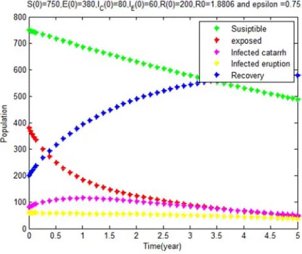
In Figure 7, simulation study shows the result of the impact of testing and therapy of exposed individual at Latent period with the rate and the reproduction number and the other parameter values are taken as mentioned above. The population dynamics of epidemic compartmental model are considered. The exposed latent individuals increase slightly to 386 initially and then decrease to 203. Also the infectives with early symptom or infected catarrh increase to 89. The infectives with later symptom or infected eruption increase to 63. Recovered persons increase to 490. Finally, the disease remains in the population at a consistent level, as one infected eruption individual transmits the disease to one susceptible.
Figure 7. Population dynamics of five compartment model.
Table 3. Comparisons of the results of and models.
S. No. ‰Š‹Œ model ‰Š‹•‹ŠŒ model
1 The human population is
divided into four compartments
The human population is divided into five compartments
2 The model has structure The model has
structure
3 Births and deaths are negligible and omitted
Birth, deaths and deaths due to disease are considered 4 The population is closed The population is not closed
5 Measles therapy test is not considered
Measles therapy test is considered
S. No. ‰Š‹Œ model ‰Š‹•‹ŠŒ model
7 Only disease free equilibrium point is analyzed
Disease free equilibrium and endemic equilibrium points are analyzed
8 Reproduction ratio is formulated
Reproduction ratio is formulated
9 Mathematical analysis is less difficult
Mathematical analysis is more difficult
10 Treatment is not considered Treatment is not considered 11 Vaccination is not used Measles therapy test is used
5. Conclusions
This study is to formulate and analyze the deterministic compartmental model for the transmission dynamics of measles disease in the human populations. The testing of measles therapy is one of the main control strategies of measles in addition to vaccination. The basic reproduction number has been computed using next generation matrix method. From the result of the stability analysis, it has been shown that the diseases free equilibrium point is locally asymptotically stable and globally asymptotically stable. Also disease endemic equilibrium points are derived and shown following Routh- Hurwitz criteria that the endemic equilibrium point is locally stable. From simulation study it can be summarized that in the present model large number of exposed individuals are transferred to recovered compartment due to Measles therapy test, and thus the propagation of the infection is controlled considerably. The simulation results in figures 3 to 7 indicate that testing, diagnosis and latent period therapy on exposed individuals will have a greater impact on the disease control. Further if the rate of exposed latent individuals increases due to Measles therapy test then the population size of exposed individuals decrease but that of the recovered individual increases steadily.
The standard model and the proposed models have been compared and the observations are presented in a tabular form showing clearly that the present model is more advantageous.
References
[1] A. Mazer Sankale. Guide de medicine en Afrique ET Ocean Indien, EDICEF, Paris 1988.
[2] Daley D. J. and Gani J. 2005. Epidemic Modeling and Introduction, New York: Cambridge University Press. [3] N. F. Britton 2003. Essential Mathematical Biology, parts of
Chapter 3: Infectious Diseases.
[4] Dancho Desaleng, Purnachandra Rao Koya. The Role of Polluted Air and Population Density in the Spread of Mycobacterium Tuberculosis Disease. Journal of Multidisciplinary Engineering Science and Technology JMEST. Vol. 2, Issue 5, May 2015, http://www.jmest.org/wp-content/uploads/JMESTN42350782.pdf
[5] A. A. Momoh, M. O. Ibrahim, I. J. Uwanta, S. B. Manga. Mathematical modeling for control of measles epidemiology. International Journal of Pure and Applied Mathematics Volume 87, No. 5, 2013, 707-718.
[6] Stephen Edward, Kitengeso Raymond E., Kiria Gabriel T., Felician Nestory, Mwema Godfrey G., Mafarasa Arbogast P. A Mathematical Model for Control and Elimination of the Transmission Dynamics of Measles. Applied and Computational Mathematics. Vol. 4, No. 6, 2015, pp. 396-408. doi: 10.11648/j.acm.20150406.12
[7] Demsis Dejene, Purnachandra Rao Koya. Population Dynamics of Dogs Subjected To Rabies Disease. Journal of Mathematics IOSR-JM, e-ISSN: 2278-5728; p-ISSN: 2319-765X. Volume 12, Issue 3, Version IV, May – June 2016, Pp 110-120 www.iosrjournals.org
[8] Tadele Degefa Bedada, Mihretu Nigatu Lemma and Purnachandra Rao Koya. Mathematical Modeling and simulation study of Influenza disease, Journal of Multidisciplinary Engineering Science and Technology JMEST. Vol. 2, Issue 11, November 2015, Pp 3263 – 69. ISSN: 3159-0040. http://www.jmest.org/wp-content/uploads/JMESTN42351208.pdf
[9] N. Chitins, J. Hyman and J. Cushing. Determining important parameters in the spread of malaria through the sensitivity analysis of a malaria model, Bull. Math. Biology, 70, 2008, 1272 - 1296.
[10] Arino J., Brauer F., Van den Driessche P., Watmough J., and Wu J. 2008. A model for influenza with vaccination and antiviral treatment, Journal of Theoretical Biology, 253, 118 -130.
[11] Anes Tawhir 2012. Modeling and Control of Measles Transmission in Ghana, Master of Philosophy thesis, Kwame Nkrumah University of Science and Technology.
[12] M. O. Fred, J. K. Sigey, J. A. Okello, J. M. Okwyo and G. J. Kang'ethe 2014. Mathematical Modeling on the Control of Measles by Vaccination: Case Study of KISII Country, Kenya. The SIJ Transactions on Computer Science Engineering and Its Applications CSEA, Vol 2, pp. 61-69.
[13] Arino J., Brauer F., van den Driessche P., Watmough J., and Wu J. 2006. Simple models for containment of a pandemic, Journal of the Royal Society Interface, 3, 453 -457.