Journal of Applied Research on Industrial
Engineering www.journal-aprie.com
A Generalized Model for Fuzzy Linear Programs with
Trapezoidal Fuzzy Numbers
Seyed Hadi Nasseri *, 1, Hadi Zavieh1, Seyedeh Maedeh Mirmohseni2 1Department of Mathematics,University of Mazandaran, Babolsar, Iran. 2
School of Mathematics and Information Science, Key Laboratory of Mathematics and Interdisciplinary Sciences of Guangdong Higher Education Institutes, Guangzhou University, Guangzhou 510006, China.
A B S T R A C T P A P E R I N F O
In this paper, a linear programming problem with symmetric trapezoidal fuzzy number which is introduced by Ganesan et al. in [4] is generalized to a general kind of trapezoidal fuzzy number. In doing so, we first establish a new arithmetic operation for multiplication of two trapezoidal fuzzy numbers. in order to prepare a method for solving the fuzzy linear programming and the primal simplex algorithm, a general linear ranking function has been used as a convenient approach in the literature. In fact, our main contribution in this work is based on 3 items: 1) Extending the current fuzzy linear program to a general kind which doesn’t essentially include the symmetric trapezoidal fuzzy numbers, 2) Defining a new multiplication role of two trapezoidal fuzzy numbers, 3) Establishing a fuzzy primal simplex algorithm for solving the generalized model. We in particular emphasize that this study can be used for establishing fuzzy dual simplex algorithm, fuzzy primal-dual simplex algorithm, fuzzy multi objective linear programming and the other similar methods which are appeared in the literature.
Chronicle:
Received: 06 June 2017 Revised:10 August 2017 Accepted:24 August 2017 Available: 24 August 2017
Keywords :
Fuzzy linear programming. Fuzzy arithmetic. Fuzzy ordering. Fuzzy primal simplex algorithm.
1. Introduction
Fuzzy mathematical programming has been developed for treating uncertainty about the setting optimization problems. In recent years, various attempts have been made to study the solution of fuzzy linear programming problems, either from theoretical or computational point of view. After the pioneering works on this area many authors have considered various kinds of the FLP problems and have proposed several approaches to solve these problems [2,3,8,9,10,13]. Some authors have made a comparison between fuzzy numbers and in particular linear ranking function to solve the fuzzy linear programming problems. Of course, ranking functions have been proposed by researchers to meet their requirements regarding the
*Corresponding author
makers to adapt to the real situations and it, in particular, can solve these problems as simple as possible.
2. Preliminaries
2.1. Definitions and notations
In this section, some notations, concepts, new definitions and some fundamental results have been presented on fuzzy arithmetic in the lake of symmetric assumption and a new generalized definition has been particularly proposed for multiplication of the general trapezoidal fuzzy numbers.
Definition 2.1. A fuzzy set 𝑎̃on ℝ is said to be a trapezoidal fuzzy number if there exists real numbers 𝑎1, 𝑎2, where 𝑎1 ≤ 𝑎2 and ℎ1, ℎ2 ≥ 0 such that
𝑎̃(𝑥) =
{ 𝑥 ℎ1+
ℎ1− 𝑎1
ℎ1 , 𝑓𝑜𝑟 𝑥 ∈ (𝑎1− ℎ1, 𝑎1) 1, 𝑓𝑜𝑟 𝑥 ∈ (𝑎1, 𝑎2) −𝑥
ℎ2
+𝑎2+ ℎ2 ℎ2
, 𝑓𝑜𝑟 𝑥 ∈ (𝑎2, 𝑎2+ ℎ2)
0, 𝑜𝑡ℎ𝑒𝑟𝑤𝑖𝑠𝑒,
where 𝑎̃(𝑥) is the membership function of fuzzy number 𝑎̃. We denoted it by 𝑎̃ = [𝑎1, 𝑎2, ℎ1, ℎ2].
In the above definition, when ℎ1 = ℎ2 we called it as ''symmetric trapezoidal fuzzy number ''. Moreover, when ℎ1 = ℎ2 = 0;𝑎̃ = [𝑎1, 𝑎2].
We use ℱ(ℝ) to denote the set of all trapezoidal fuzzy numbers.
Definition 2.2. Let 𝑎̃ = [𝑎1, 𝑎2, ℎ1, ℎ2] and 𝑏̃ = [𝑏1, 𝑏2, 𝑘1, 𝑘2] be two trapezoidal fuzzy numbers. If so, the arithmetic operations on 𝑎̃ and 𝑏̃will be defined by:
(i) Addition: 𝑎̃ + 𝑏̃ = [𝑎1, 𝑎2, ℎ1, ℎ2] + [𝑏1, 𝑏2, 𝑘1, 𝑘2] = [𝑎1+ 𝑏1, 𝑎2+ 𝑏2, ℎ1+ 𝑘1, ℎ2+ 𝑘2].
(ii) Subtraction:𝑎̃ − 𝑏̃ = [𝑎1, 𝑎2, ℎ1, ℎ2] − [𝑏1, 𝑏2, 𝑘1, 𝑘2] = [𝑎1− 𝑏2, 𝑎2− 𝑏1, ℎ1+ 𝑘2, ℎ2+ 𝑘1].
2.2. Ranking functions
for ordering the elements of ℱ(ℝ) is to define a ranking function ℛ: ℱ(ℝ) ⟶ ℝ which maps each fuzzy number into the real line, where a natural order exists.
Definition 2.3. We defined orders on ℱ(ℝ) by 𝑎̃ ≽ 𝑏̃ if and only if ℛ(𝑎̃) ≥ ℛ(𝑏̃),
𝑎̃ ≻ 𝑏̃ if and only if ℛ(𝑎̃) ≻ ℛ(𝑏̃), 𝑎̃ ≃ 𝑏̃ if and only if ℛ(𝑎̃) ≃ ℛ(𝑏̃),
where 𝑎̃ and b̃ are in ℱ(ℝ). Also we write 𝑎̃ ≼ 𝑏̃ if and only if 𝑏̃ ≽ 𝑎̃.
Attention has been exclusively paid to linear ranking functions, that is, a ranking function ℛ such that:
ℛ(𝑘𝑎̃ + 𝑏̃) = 𝑘ℛ(𝑎̃) + ℛ(𝑏̃)
for any 𝑎̃ and 𝑏̃ belonging to ℱ(ℝ) and any k ∈ ℝ.
Now using the above approach, we may rank a big category of fuzzy numbers, where the symmetric property is extended to the non-symmetric form, too.
Remark 1. For any trapezoidal fuzzy number 𝑎̃, the relation 𝑎̃ ≽ 0̃holds, if there exists 𝜀 > 0 and 𝛼 > 0 such that 𝑎̃ ≽ (−𝜀, 𝜀, 𝛼, 𝛼). We realized that ℛ(−𝜀, 𝜀, 𝛼, 𝛼) = 0. We also considered 𝑎̃ ≈ 0̃ only if ℛ(𝑎̃) = 0. Thus, without loss of generality, throughout the paper, we regard 0̃ = (0, 0, 0, 0)as the zero trapezoidal fuzzy number.
The following lemma is now immediately at hand.
Lemma 2.1. Let ℛ be any linear ranking function. Then,
(i) 𝑎̃ ≽ 𝑏̃ if and only if 𝑎̃ − 𝑏̃ ≽ 0̃ if and only if −𝑏̃ ≽ −𝑎̃, (ii) If 𝑎̃ ≽ 𝑏̃ and 𝑐̃ ≽ 𝑑̃ then 𝑎̃ + 𝑐̃ ≽ 𝑏̃ + 𝑑̃.
The linear ranking function has been considered on ℱ(ℝ) as ℛ(𝑎̃) = 𝑐𝑙𝑎𝑙 + 𝑐
𝑢𝑎𝑢+ 𝑐𝛼𝛼 + 𝑐𝛽𝛽,
where 𝑎̃ = (𝑎𝑙, 𝑎𝑢, 𝛼, 𝛽), and 𝑐
𝑙, 𝑐𝑢, 𝑐𝛼, 𝑐𝛽 are constants, at least one of them is nonzero. A
Proposition 2.1. For any trapezoidal fuzzy numbers 𝑎̃, 𝑏̃ and 𝑐̃, we have
(i) 𝑐̃ (𝑎̃ + 𝑏̃) ≈ (𝑐̃ 𝑎̃ + 𝑐̃ 𝑏̃),
(ii) 𝑐̃ (𝑎̃ − 𝑏̃) ≈ (𝑐̃ 𝑎̃ − 𝑐̃ 𝑏̃).
Theorem 2.1. (i) The relation ≼ is a partial order relation on the set of trapezoidal fuzzy
numbers.
(ii) The relation ≼ is a linear order relation on the set of trapezoidal fuzzy numbers.
(iii) For any two trapezoidal fuzzy numbers 𝑎̃ and 𝑏̃; if 𝑎̃ ≼𝑏̃, then 𝑎̃ ≼ (1 − 𝜆)𝑎̃ + 𝜆𝑏̃ ≼ 𝑏̃,
for all λ, 0 ≤ λ ≤ 1.
3. A new role in fuzzy arithmetic and fuzzy ordering
A definition of the multiplication of two symmetric fuzzy numbers is given by Ganesan and Veeramani in [7] based on the Extension Principle (see [12]). However, fuzzy arithmetic and a fuzzy ordering role based on the given definition, is established by many researchers. Although many valuable works are appeared in the literature, there are a big limitation in the basic definition. In fact, the symmetric assumption is not reasonable in practice since there are many real situations that need to be dealt with by decision makers, especially when the main parameters of the system is formulated in the more general case and frankly in the form of non-symmetric fuzzy number. Moreover, by introducing a new definition of the length of 𝜔 , we may keep the length of the resulted fuzzy number which is obtained based on the given multiplication role.
For defining the multiplication of the two (non-symmetric) trapezoidal fuzzy numbers, we first needed to define the following notations:
Let
𝜃 = {𝑎1𝑏1, 𝑎1𝑏2, 𝑎2𝑏1, 𝑎2𝑏2}, 𝛾 = 𝐴𝑣𝑒𝑟𝑎𝑔𝑒 𝜃.
Then, define
𝛼 = | 𝛾 − 𝑚𝑖𝑛𝜃 | and 𝛽 = |𝑚𝑎𝑥𝜃 − 𝛾|. Let 𝜔 = |𝛽−𝛼
2 | and we now may define the multiplication of two non-symmetric trapezoidal
Definition 3.1. Let 𝑎̃ = [𝑎1, 𝑎2, ℎ1, ℎ2] and 𝑏̃ = [𝑏1, 𝑏2, 𝑘1, 𝑘2] be two trapezoidal fuzzy numbers. Then the arithmetic operations on 𝑎̃ and 𝑏̃are given by:
Multiplication: 𝑎̃𝑏̃ = [𝑎1, 𝑎2, ℎ1, ℎ2][𝑏1, 𝑏2, 𝑘1, 𝑘2]
= [(𝑎1+ 𝑎2
2 ) (
𝑏1+ 𝑏2
2 ) − 𝜔, (
𝑎1+ 𝑎2
2 ) (
𝑏1+ 𝑏2
2 ) + 𝜔, |𝑎2𝑘1+ 𝑏2ℎ1|, |𝑎2𝑘2+ 𝑏2ℎ2| ].
From the above definition, it is clear that
𝜆𝑎̃={[𝜆𝑎1, 𝜆𝑎2, 𝜆ℎ1, 𝜆ℎ2], 𝑓𝑜𝑟 𝜆 ≥ 0, [𝜆𝑎2, 𝜆𝑎1, −𝜆ℎ2, −𝜆ℎ1], 𝑓𝑜𝑟 𝜆 < 0.
Remark 2. Depending upon the need, we overcame the limitation of the multiplication role which is given just for the symmetric kind of trapezoidal fuzzy numbers. See in [4]
Definition 3.2.The model
𝑚𝑎𝑥 𝑧̃ = ∑𝑛𝑗=1𝑐̃𝑥𝑗̃𝑗
(2-1)
𝑆. 𝑡: ∑ 𝑎𝑖𝑗𝑥̃𝑗 𝑛
𝑗=1
≼ 𝑏̃ , 𝑖 = 1, … , 𝑚 𝑖
𝑥̃𝑗 ≽0 ̃ , 𝑗 = 1, … , 𝑛
if 𝑎𝑖𝑗 ∈ ℝ, and 𝑐̃, 𝑥𝑗 ̃ , 𝑏𝑗 ̃ ∈ ℱ(ℝ),𝑖 𝑖 = 1, … , 𝑚, 𝑗 = 1, … , 𝑛 is called a Semi-Fuzzy Linear Programming (SFLP) problem.
Definition 3.3. Any 𝑋̃ = (𝑥̃, 𝑥1 ̃, … , 𝑥2 ̃ ) ∈ ℱ𝑛 𝑛(ℝ), where each 𝑥 𝑖
̃ ∈ ℱ(ℝ), which satisfies the constraints and non-negativity restrictions of (2-1) is said to be a fuzzy feasible solution to (2-1).
Definition 3.4. Let Q be the set of all fuzzy feasible solutions of (1). A fuzzy feasible solution 𝑋̃ ∈ 𝑄𝑜 is said to be a fuzzy optimum solution to (1), if 𝐶̃𝑋̃ ≽ 𝐶̃𝑋̃𝑜 for all 𝑋̃ ∈ 𝑄, where 𝐶̃ = (𝑐̃ , 𝑐1 ̃ , … , 𝑐2 ̃ )𝑛 and 𝐶̃𝑋̃ = 𝑐̃ 𝑥1̃ + 𝑐1 ̃ 𝑥2̃ + ⋯ + 𝑐2 ̃𝑥𝑛̃𝑛.
3.2. Fuzzy Basic feasible solution
The concept of fuzzy basic feasible solution is similar to the given definition in [8]. We give a new definition for fuzzy solution associated to the discussed model as below:
Definition 3.5. Let 𝑋̃ = (𝑥̃, 𝑥1 ̃, … , 𝑥2 ̃ ) ∈ ℱ𝑛 𝑛(ℝ), suppose that 𝑥̃ = (𝑥̃
[−𝛼𝑗, 𝛼𝑗, ℎ𝑗, ℎ𝑗] for some 𝛼𝑖 > 0, ℎ𝑗 and ℎ𝑗 ≥ 0 that is 𝑥̃ ≈ 0̃𝑗 and every basic variable of the corresponding to every feasible basic 𝐵 is positive , 𝑥̃ is said to be a degenerated fuzzy basic feasible solution .
The following theorem concerns the so-called nondegenerate FNLP problems,
Theorem 3.1. Let the FNLP problem be nondegenerate. A basic feasible solution 𝑥̃ ≈𝐵 𝐵−1𝑏̃, 𝑥
𝑁
̃ ≈ 0̃ is optimal to (2-1) only if 𝑧̃ ≽ 𝑐𝑗 ̃𝑗 for all 𝑗, 1 ≤ 𝑗 ≤ 𝑛.
Proof: Suppose that 𝑥̃ = (𝑥̃∗ 𝐵𝑇 , 𝑥̃
𝑁𝑇)𝑇 is a basic feasible solution to (2-1), where 𝑥̃ ≈𝐵 𝐵−1𝑏̃, 𝑥
𝑁
̃ ≈ 0̃. Then, 𝑧̃ = 𝑐̃𝑥𝐵̃ = 𝑐𝐵 ̃𝐵𝐵 −1𝑏̃. On the other hand, for every feasible solution 𝑥̃ ,
we have 𝑏̃ ≈ 𝐴𝑥̃ ≈ 𝐵𝑥̃ + 𝑁𝑥𝐵 ̃.𝑁 Hence, we obtain: 𝑧̃ = 𝑐̃𝑥̃ − ∑ (𝑧̃ − 𝑐𝑗 ̃)𝑥𝑗 ̃𝑗
𝑗≠𝐵𝑖
. (3 − 1)
Then,
𝑧̃ = 𝑧̃ = 𝑐∗ ̃𝑥𝐵̃ + 𝑐𝐵 ̃𝑥𝑁̃ = 𝑐𝑁 ̃𝐵𝐵 −1𝑏̃ − ∑ (𝑐 𝐵 ̃𝐵−1𝑎
𝑗− 𝑐̃)𝑥𝑗 ̃𝑗 𝑗≠𝐵𝑖
The proof can now be completed using (3-1) and Theorem 3.2 given in Section 3.
Now we are going to devise a fuzzy primal simplex algorithm for solving the Problem (2-1).
3.3. Primal simplex method in tableau format for the fuzzy linear Problems
Consider the fuzzy linear programing problem as in (2-1). We rewrite the fuzzy linear programing problem as:
𝑀𝑎𝑥 𝑧̃ = 𝑐̃𝑥𝐵̃ + 𝑐𝐵 ̃𝑥𝑁̃𝑁
𝑠. 𝑡. 𝐵𝑥̃ + 𝑁𝑥𝐵 ̃ = 𝑏̃𝑁
𝑥̃ ≽ 0̃, 𝑥𝐵 ̃ ≽ 0̃.𝑁
Hence we have 𝑥̃ + 𝐵𝐵 −1𝑁𝑥 𝑁
̃ ≈ 𝐵−1𝑏̃. Therefore, 𝑧̃ + (𝑐 𝐵
̃𝐵−1𝑁 − 𝑐 𝑁
̃)𝑥̃ ≈ 𝑐𝑗 ̃𝐵𝐵 −1𝑏̃. With 𝑥̃ ≈ 0̃𝑁 we have 𝑥̃ = 𝐵𝐵 −1𝑏̃ ≈ 𝑦
𝑜
̃, and 𝑧̃ ≈ 𝑐̃𝐵𝐵 −1𝑏̃. Thus we rewrited the above problem as
in Table 1.
Table 1. The primal simplex tableau.
Basis 𝑥̃ 𝑥𝐵 ̃ 𝑁 R.H.S 𝑧̃ 0̃ 𝑧̃ − 𝑐𝑁 ̃ = 𝑐𝑁 ̃𝐵𝐵 −1𝑁 − 𝑐
𝑁
̃ 𝑦̃ = 𝑐𝑜𝑜 ̃𝐵𝐵 −1𝑏̃
Remark 3. Table 1 gives all the information needed to proceed with the simplex method. The fuzzy cost row in Table 1 is 𝑦̃𝑜𝑇= 𝑐
𝐵
̃𝐵−1𝐴 − 𝑐̃, where 𝑦̃
𝑜𝑗 = 𝑐̃𝐵𝐵 −1𝑎𝑗− 𝑐̃ = 𝑧𝑗 ̃ − 𝑐𝑗 ̃, 1 ≤ 𝑗 ≤𝑗
𝑛, with 𝑦̃𝑜𝑗 ≈ 0̃ for 𝑗 = 𝐵𝑖, 1 ≤ 𝑖 ≤ 𝑚. According to the optimality conditions (Theorem 3.1), we are at the optimal solution if 𝑦̃𝑜𝑗 ≽ 0̃ for all 𝑗 ≠ 𝐵𝑖, 1 ≤ 𝑖 ≤ 𝑚. On the other hand, if 𝑦̃𝑜𝑗 ≼ 0̃ for some 𝑘 ≠ 𝐵𝑖, 1 ≤ 𝑖 ≤ 𝑚, the problem is either unbounded or an exchange of a basic variable 𝑥̃𝐵𝑟 and the nonbasic variable 𝑥̃𝑘 can be made to increase the rank of the objective value (under nondegeneracy assumption). The following results established in [9] help us devise the fuzzy primal simplex algorithm.
Theorem 3.2. If there is a column 𝑘 (not in basis) in a fuzzy primal simplex tableau as 𝑦̃ =𝑜𝑘 𝑧𝑘
̃ − 𝑐̃ ≺ 0̃𝑘 and 𝑦𝑖𝑘 ≤ 0, 1 ≤ 𝑖 ≤ 𝑚, the problem (2-1) is unbounded.
Theorem 3.3. If a nonbasic index 𝑘exists in a fuzzy primal simplex tableau like 𝑦̃ = 𝑧𝑜𝑘 ̃ −𝑘 𝑐̃ ≺ 0̃𝑘 and there exists a basic index 𝐵𝑖 like 𝑦𝑖𝑘 ≥ 0 , a pivoting row 𝑟can be found so that pivoting on 𝑦𝑟𝑘 can yield a feasible tableau with a corresponding nondecreasing (increasing
under nondegeneracy assumption) fuzzy objective value.
Remark 4 (see [9]). If there exists k such that 𝑦̃ ≺ 0̃𝑜𝑘 and the problem is not unbounded, r can be chosen as
𝑦̃𝑟𝑜
𝑦𝑟𝑘 = 𝑚𝑖𝑛1≤𝑖≤𝑚{ 𝑦̃𝑖𝑜
𝑦𝑖𝑘 , 𝑦𝑖𝑘 > 0},
Where it is the minimum fuzzy value of the above ratio.
in order to replace 𝑥̃𝐵𝑟 in the basis by 𝑥̃𝑘, resulting in a new basis 𝐵 = (𝑎𝐵𝑖, 𝑎𝐵2, … , 𝑎𝐵𝑟−1, 𝑎𝑘, 𝑎𝐵𝑟+1, … , 𝑎𝐵𝑚). The new basis is primal feasible and the corresponding fuzzy objective value is nondecreasing (increasing under nondegeneracy assumption). It can be shown that the new simplex tableau is obtained by pivoting on 𝑦𝑟𝑘, i.e. doing Gaussian elimination on the 𝑘 th column by using the pivot row 𝑟, with the pivot 𝑦𝑟𝑘, to transform the 𝑘 th column to the unit vector 𝑒𝑟. It is easily seen that the new fuzzy objective value is: 𝑦̂̃ = 𝑦𝑜𝑜 ̃ − 𝑦𝑜𝑜 ̃𝑜𝑘
𝑦𝑟𝑜
𝑦𝑟𝑘 ≽ 𝑦̃𝑜𝑜 where 𝑦̃𝑜𝑘 ≼ 0̃ and
𝑦𝑟𝑜
𝑦𝑟𝑘 (if the problem is nondegenerate, and consequently 𝑦𝑟𝑜
𝑦𝑟𝑘 > 0 and hence𝑦̂̃ ≈ 𝑦𝑜𝑜 ̃𝑜𝑜). We now describe the pivoting strategy.
3.4. Pivoting and change of basis
1) Divide row r by 𝑦𝑟𝑘.
2) For 𝑖 = 0,1, . . . , 𝑚 and 𝑖 ≠ 𝑟, update the 𝑖 th row by adding to it −𝑦𝑖𝑘 times the new 𝑟th row.
We now present the primal simplex algorithm for the FNLP problem.
3.5. The main steps of fuzzy primal simplex algorithm
Algorithm 3.1: The fuzzy primal simplex method
Assumption: A basic feasible solution with basis B and the corresponding simplex tableau is
at hand.
1. The fuzzy basic feasible solution is given by 𝑥̃ =𝐵 𝑦̃𝑜 = 𝐵−1𝑏̃ and 𝑥̃ ≈ 0̃𝑁 The fuzzy objective value is: 𝑧̃ = 𝑦̃ = 𝑐𝑜𝑜 ̃𝐵𝐵 −1𝑏̃.
2. Calculate 𝑦̃𝑜𝑗 = 𝑧̃ − 𝑐𝑗 ̃, 1 ≤ 𝑗 ≤ 𝑛,𝑗 with for 𝑗 ≠ 𝐵𝑖, 1 ≤ 𝑖 ≤ 𝑚.
Let 𝑦̃ = 𝑚𝑖𝑛𝑜𝑘 1≤𝑗≤𝑛{𝑦̃ }𝑜𝑗 . If 𝑦̃ ≽ 0̃𝑜𝑘 , then stop; the current solution is optimal.
3. If 𝑦̃ ≼ 0̃𝑜𝑘 , then stop; the problem is unbounded. Otherwise, it determines an index 𝑟 corresponding to a variable 𝑥̃𝐵𝑟 leaving the basis as follows:
𝑦̃𝑟𝑜 𝑦𝑟𝑘
= 𝑚𝑖𝑛1≤𝑖≤𝑚{𝑦̃𝑖𝑜 𝑦𝑖𝑘
, 𝑦𝑖𝑘 > 0}.
4. Pivot on and update the simplex tableau. Go to step 2.
Remark 5 (limitation of existing method). Investigation of the current models and methods
show that almost all of them are disable to formulate the real problems when the symmetric assumption is not at hand. Furthermore, by defining a new product role, we may to define a practical method for solving the generalized model, while the methods cannot work by the pioneering approach.
Now we are on the point of giving some illustrative examples. In the next subsection, we give two examples. The first problem is concerning to the symmetric form of fuzzy number that discussed by Ganesan et al. in [4]. This example shows how we can solve the existing shortcomings of the first model which is given in Example 3.1.
3.6. Numerical examples
Example 3.1. We consider the fuzzy mathematical model which is given by Ganesan et al.
in [4]. The corresponding model is given in the below.
𝑚𝑎𝑥 𝑍̃ ≈ [13, 15, 2, 2] 𝑥̃1+ [12, 14, 3, 3] 𝑥̃2 + [15, 17, 2, 2] 𝑥̃3
𝑠𝑢𝑏𝑗𝑒𝑐𝑡 𝑡𝑜 12𝑥̃1 + 13𝑥̃2 + 12𝑥̃3≼ [475, 505, 6, 6],
14𝑥̃1 + 13𝑥̃3 ≼ [460, 480, 8, 8],
12𝑥̃1 + 15 𝑥̃2 ≼ [465, 495, 5, 5]
𝑥̃1 ≽ 0̃, 𝑥̃2 ≽ 0̃, 𝑥̃3 ≽ 0̃
Now the standard form of the fuzzy linear programming problem becomes,
𝑚𝑎𝑥 𝑍̃ ≈ [13, 15, 2, 2] 𝑥̃1+ [12, 14, 3, 3] 𝑥̃2 + [15, 17, 2, 2] 𝑥̃3
𝑠𝑢𝑏𝑗𝑒𝑐𝑡 𝑡𝑜 12𝑥̃1 + 13𝑥̃2 + 12𝑥̃3+ 𝑠̃1 ≈ [475, 505, 6, 6],
14𝑥̃1 + 13𝑥̃3+ 𝑠̃2 ≈ [460, 480, 8, 8],
12𝑥̃1 + 15 𝑥̃2+ 𝑠̃3 ≈ [465, 495, 5, 5]
𝑥̃1 ≽ 0̃, 𝑥̃2 ≽ 0̃, 𝑥̃3 ≽ 0̃
Using the multiplication role which is established by Ganesan et al., the fuzzy optimal solution and the fuzzy optimal value of objective function is as follows:
𝑥̃1= [0,0,0,0], 𝑥̃2= [ 415 169,
1045 169 ,
174 169,
174
169], 𝑥̃3= [ 460
13 , 480
13 , 8 13,
8 13],
𝑠̃1= [0,0,0,0], 𝑠̃2= [0,0,0,0] , 𝑠̃3= [ 62910
169 , 77430
169 , 3455
169 , 3455
169].
𝑍̃𝑉= [ 94235
169 ,
120265 169 ,
19819 169 ,
19819 169 ].
Using a ranking function such as Yager, we obtain 𝑅(𝑍̃𝑉) = 𝟏𝟎𝟕𝟐𝟓𝟎
𝟏𝟔𝟗 .
By substituting the fuzzy values of 𝑥̃2 and 𝑥̃3 in the objective function and using the new role
of fuzzy multiplication, we have:
𝑍̃𝐻 = 𝑐̃1𝑥̃1+ 𝑐̃2𝑥̃2+ 𝑐̃3𝑥̃3
𝑐̃1𝑥̃1= [13, 15, 2, 2][0, 0, 0, 0]=[0, 0, 0, 0]
𝑐̃2𝑥̃2= [ 415 169,
1045 169 ,
174 169,
174
169] [12,14,3,3] = [ 9175
169 , 9805
169 , 5571
169 , 5571
𝑐̃3𝑥̃3= [15,17,2,2] [ 460
13 , 480
13 , 8 13,
8 13] = [
97630 169 ,
97890 169 ,
1096 169 ,
1096 169]
𝑍̃𝐻= [0, 0, 0, 0]+[ 9175
169 , 9805
169 , 5571
169 , 5571
169] + [ 97630
169 , 97890
169 ,
14248
169 , 14248
169 ]
= [106805 169 ,
107695 169 ,
19819
169 , 19819
169 ]
We clearly obtain 𝑅(𝑍̃𝐻) =
𝟏𝟎𝟕𝟐𝟓𝟎
𝟏𝟔𝟗 .
So, according to the ordering role which is given in Definition 2.2, it is concluded that 𝑍̃𝑉 ≈ 𝑍̃𝐻
In fact, it has been shown ,in this example, that the proposed method can solve the symmetric version of the given fuzzy numbers as well as Ganesan’s method.
Example 3.2 In this example, we consider a general form of trapezoidal fuzzy number for
coefficients in the objective function, if it is not necessary to be symmetric. 𝑚𝑎𝑥 𝑍̃ ≈ [13, 15, 3, 4] 𝑥̃1+ [12, 14, 4, 5] 𝑥̃2 + [15, 17, 3, 4] 𝑥̃3
𝑠𝑢𝑏𝑗𝑒𝑐𝑡 𝑡𝑜 12𝑥̃1 + 13𝑥̃2 + 12𝑥̃3≼ [475, 505, 6, 6],
14𝑥̃1 + 13𝑥̃3 ≼ [460, 480, 8, 8],
12𝑥̃1 + 15 𝑥̃2 ≼ [465, 495, 5, 5]
𝑥̃1 ≽ 0̃, 𝑥̃2 ≽ 0̃, 𝑥̃3≽ 0̃
Now the standard form of the fuzzy linear programming problem becomes 𝑚𝑎𝑥 𝑍̃ ≈ [13, 15, 3, 4] 𝑥̃1+ [12, 14, 4, 5] 𝑥̃2 + [15, 17, 3, 4] 𝑥̃3
𝑠𝑢𝑏𝑗𝑒𝑐𝑡 𝑡𝑜 12𝑥̃1 + 13𝑥̃2 + 12𝑥̃3+ 𝑥̃4≈ [475, 505, 6, 6],
14𝑥̃1 + 13𝑥̃3+ 𝑥̃5 ≈ [460, 480, 8, 8],
12𝑥̃1 + 15 𝑥̃2+ 𝑥̃6 ≈ [465, 495, 5, 5],
𝑥̃1 ≽ 0̃, 𝑥̃2 ≽ 0̃, 𝑥̃3 ≽ 0̃.
The first tableau of the fuzzy primal simplex algorithm is given as below:
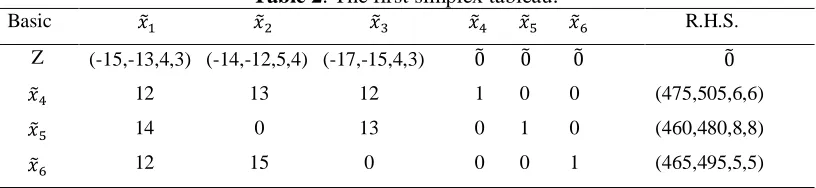
Table 2. The first simplex tableau.
Basic 𝑥̃1 𝑥̃2 𝑥̃3 𝑥̃4 𝑥̃5 𝑥̃6 R.H.S.
Z (-15,-13,4,3) (-14,-12,5,4) (-17,-15,4,3) 0̃ 0̃ 0̃ 0̃ 𝑥̃4
𝑥̃5
𝑥̃6
12 13 12 1 0 0 14 0 13 0 1 0 12 15 0 0 0 1
The first Since (𝑦̃01, 𝑦̃02, 𝑦̃03) = ((−15, −13,4,3), (−14, −12,5,4), (−17, −15,4,3)), and (ℛ(𝑦̃01), ℛ(𝑦̃02), ℛ( 𝑦̃03)) = (−14.25, −13.25, −16.25), then 𝑥̃3 inters the basis and based on the minimum ratio test, the leaving variable is 𝑥̃5 . Pivoting on 𝑦53 = 13.
After calculating the amount of R.H.S. column in Table 1,it has been found that the multiplication role which was defined by Ganesan and Veeramani in [4] is not satisfying and we must hence use Definition 2.2 for obtaining the amount of multiplication as follows:
𝑦𝑜𝑜𝑛𝑒𝑤 = 0̃ + (460 13, 480 13, 8 13, 8 13)(15,17,3,4)
Now, assume that 𝑎̃ = (460 13, 480 13, 8 13, 8
13) and 𝑏̃ =(15,17,3,4), then 𝜃 = {𝑎1𝑏1, 𝑎1𝑏2, 𝑎2𝑏1, 𝑎2𝑏2} = {6900
13 , 7820 13 , 7200 13 , 8160 13 }, 𝛾 = 𝐴𝑣𝑒𝑟𝑎𝑔𝑒 𝜃 =7520
13 .
𝛼 = | 𝛾 − 𝑚𝑖𝑛𝜃 | =620
13 , 𝛽 = |𝑚𝑎𝑥𝜃 − 𝛾| = 640
13.
So, 𝜔 = |𝛽−𝛼
2 | =
10 13 . 𝑎̃𝑏̃ = [(𝑎1+ 𝑎2
2 ) (
𝑏1+ 𝑏2
2 )− 𝜔,(
𝑎1+ 𝑎2
2 ) (
𝑏1+ 𝑏2
2 )+ 𝜔,|𝑎2𝑘1+ 𝑏2ℎ1|,|𝑎2𝑘2 + 𝑏2ℎ2|]
= [7510 13 , 7530 13 , 1576 13 , 2056 13 ].
Updating the data is based on the about calculation concluded in Table 2:
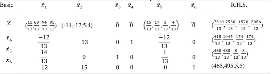
Table 3. The second simplex tableau.
Basic 𝑥̃1 𝑥̃2 𝑥̃3 𝑥̃4 𝑥̃5 𝑥̃6 R.H.S.
Z (15
13, 69 13, 94 13, 95
13) (-14,-12,5,4) 0̃ 0̃ (
15 13, 17 13, 3 13, 4 13) 0̃ (
7510 13 , 7530 13 , 1576 13 , 2056 13 ) 𝑥̃4 𝑥̃3 𝑥̃6 −12 13 13 0
14 13 0 1
12 15 0
1 −12
13 0
0 1
13 0
0 0 1
Since the problem is maximization, the optimality condition is not valid and hence 𝑥̃2 enters
the basis and the leaving variable is 𝑥̃4 . The next tableau based on the following calculations is shown in Table 3.
𝑦𝑜𝑜𝑛𝑒𝑤 = ( 7510 13 , 7530 13 , 1576 13 , 2056 13 ) + (
415 169, 1045 169, 174 169, 174 169)(12,14,4,5).
We suppose that 𝑎̃ = (415 169, 1045 169, 174 169, 174
169) and 𝑏̃ =(12,14,4,5), then 𝜃 = {𝑎1𝑏1, 𝑎1𝑏2, 𝑎2𝑏1, 𝑎2𝑏2} = {4980
169 , 12540 169 , 5810 169 , 14630 169 }, 𝛾 = 𝐴𝑣𝑒𝑟𝑎𝑔𝑒 𝜃 =9490
169, 𝛼 = | 𝛾 − 𝑚𝑖𝑛𝜃 | =4510
169 , 𝛽 = |𝑚𝑎𝑥𝜃 − 𝛾| = 5140
169.
Hence,
𝜔 = |𝛽−𝛼
2 | =
315 169 .
Then, 𝑎̃𝑏̃ = [(𝑎1+𝑎2
2 ) ( 𝑏1+𝑏2
2 )− 𝜔,( 𝑎1+𝑎2
2 ) ( 𝑏1+𝑏2
2 )+ 𝜔,|𝑎2𝑘1+ 𝑏2ℎ1|,|𝑎2𝑘2+ 𝑏2ℎ2|] = [ 18600 169 , 19230 169 , 6616 169 , 7661
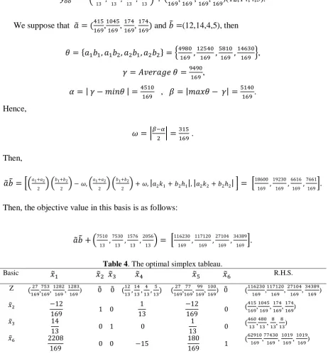
169]. Then, the objective value in this basis is as follows:
𝑎̃𝑏̃+ (7510 13 , 7530 13 , 1576 13 , 2056 13) = [
116230 169 , 117120 169 , 27104 169 , 34389 169 ].
Table 4. The optimal simplex tableau.
Basic 𝑥̃1 𝑥̃2 𝑥̃3 𝑥̃4 𝑥̃5 𝑥̃6 R.H.S.
Z (27
169, 753 169, 1282 169, 1283
169) 0̃ 0̃ (
12 13, 14 13, 4 13, 5 13) ( 27 169, 77 169, 99 169, 100 169) 0̃ (
116230 169 , 117120 169 , 27104 169 , 34389 169 ) 𝑥̃2 𝑥̃3 𝑥̃6 −12 169 1 0 14 13 0 1 2208 169 0 0 1 13 −12 169 0
0 1
13 0
−15 180
169 1
(415 169, 1045 169, 174 169, 174 169) (460 13, 480 13, 8 13, 8 13) (62910 169 , 77430 169 , 1019 169, 1019 169)
𝑥̃2∗ = (415
169, 1045
169, 174 169,
174 169), 𝑥̃3
∗ = (460
13, 480
13, 8 13,
8 13), 𝑥̃6
∗= (62910
169 ,
77430
169 ,
1019 169,
1019 169)
and 𝑥̃1∗ = 𝑥̃4∗ = 𝑥̃5∗ = 0̃, and
𝑧
∗=
(116230169 ,
117120
169 ,
27104
169 ,
34389
169 ).
Where
𝑍𝐻= [13, 15, 3, 4]𝑥̃1∗+ [12, 14, 4, 5]𝑥̃2∗ + [15, 17, 3, 4]𝑥̃3∗
= [13, 15, 3, 4]0̃ + (12,14,4,5) (415
169, 1045
169 , 174 169,
174
169) + (15,17,3,4) ( 460
13 , 480
13 , 8 13,
8 13)
= (116230 169 ,
117120 169 ,
27104 169 ,
34389 169 )
Thus, it has been seen that the proposed approach gave the same results as the mentioned problem in the method proposed by Ganesan et al. In particular, the proposed arithmetic allows the decision makers to model as a general type, where the promoters can be formulated as a general from of trapezoidal fuzzy numbers which is more appropriate for real situations than just in the symmetric form.
4. Conclusion
In the paper, a new role for the multiplication of two general forms of trapezoidal fuzzy numbers has been defined. In particular, we saw that the new model sounds to be more appropriate for the real situation, while in the pioneering model which was suggested by Ganessan et al., [4] and subsequently Das et all [1], the trapezoidal fuzzy numbers are assumed to be essential in the symmetric form. Therefore, these tools can be useful for preparing some solving algorithms, fuzzy primal, dual simplex algorithms and so on.
5. Acknowledgment
The authors would like to thanks the anonymous referees for their valuable comments to lead us for improving the earlier version of the mentioned manuscript.
References
[1] Das, S. K., Mandal, T., & Edalatpanah, S. A. (2017). A mathematical model for solving fully fuzzy linear programming problem with trapezoidal fuzzy numbers. Applied Intelligence, 46(3), 509-519.
[3] Ebrahimnejad, A., Nasseri, S. H., Lotfi, F. H., & Soltanifar, M. (2010). A primal-dual method for linear programming problems with fuzzy variables. European Journal of Industrial Engineering, 4(2), 189-209. [4] Ganesan, K., & Veeramani, P. (2006). Fuzzy linear programs with trapezoidal fuzzy numbers. Annals of
Operations Research, 143(1), 305-315.
[5] Lotfi, F. H., Allahviranloo, T., Jondabeh, M. A., & Alizadeh, L. (2009). Solving a full fuzzy linear programming using lexicography method and fuzzy approximate solution. Applied Mathematical Modelling, 33(7), 3151-3156.
[6] Klir, G., & Yuan, B. (1995). Fuzzy sets and fuzzy logic :Theory and Applications, Prentice-Hall, PTR, New Jersey.
[7] Kumar, A., Kaur, J., & Singh, P. (2011). A new method for solving fully fuzzy linear programming problems. Applied Mathematical Modelling, 35(2), 817-823.
[8] Mahdavi-Amiri, N., & Nasseri, S. H. (2007). Duality results and a dual simplex method for linear programming problems with trapezoidal fuzzy variables. Fuzzy sets and systems, 158(17), 1961-1978. [9] Mahdavi-Amiri, N., & Nasseri, S. H. (2006). Duality in fuzzy number linear programming by use of a
certain linear ranking function. Applied Mathematics and Computation, 180(1), 206-216.
[10]Maleki, H. R., Tata, M., & Mashinchi, M. (2000). Linear programming with fuzzy variables. Fuzzy sets and systems, 109(1), 21-33.
[11]Nasseri, S. H., & Ebrahimnejad, A. (2010). A fuzzy dual simplex method for fuzzy number linear programming problem. Advances in Fuzzy Sets and Systems, 5(2), 81-95.
[12]Nasseri, S. H., & Ebrahimnejad, A. (2010). A fuzzy primal simplex algorithm and its application for solving flexible linear programming problems. European Journal of Industrial Engineering, 4(3), 372-389.
[13]Nasseri, S. H., Ebrahimnejad, A., & Mizuno, S. (2010). Duality in fuzzy linear programming with symmetric trapezoidal numbers. Applications and Applied Mathematics, 5(10), 1467-1482.
[14]Yager, R. R. (1981). A procedure for ordering fuzzy subsets of the unit interval. Information sciences,