Map-Reduced Tighter Upper Bound For High
Average Utility Pattern Mining For Big Data
R.Vasumathi, Dr.S.Murugan
Abstract: High utility itemset mining is gaining momentum in the field of data mining techniques. The problem of high utility itemset mining is an extension of the problem from the frequent itemset mining. Frequent itemset mining is a well-liked problem in the data mining task which considers finding the frequent patterns in the database. Several algorithms are proposed to mine the high utility itemsets. In this paper, we proposed a method high average utility itemset mining in big data. The number of distinct items and the size of the databases are both too large. Hence, two new tighter upper bounds are used to reduce the irrelevant itemset in the database. We try to implement a new algorithm, two new tighter upper bounds for high average utility pattern mining using map reduced algorithm to reduce the search space and processing time. Experiments conducted on real-time server data sets and compare various parameters with the existing algorithms.
Index Terms: Data Mining, Frequent Itemset Mining, Association Rule Mining, High Utility Itemset Mining, Big Data. ————————————————————
1. I
NTRODUCTION:
Data mining techniques are used to find the useful information from a large database and is called knowledge discovery in database (KDD)[1],[7]. Association Rule Mining and Frequent itemset mining are basic operations in data mining [4]. Infrequent itemset mining and the association, rule mining was a principal concern in data mining and applied in real-life applications [9]. Frequent itemset mining techniques depends on the support and confidence framework where the frequency of items should be greater than the minimum support threshold [1],[2]&[8]. High utility itemset mining identifies the itemsets where item utility satisfies a given threshold value [3]. Big Data is a collection of a large dataset that cannot be processed using traditional computing techniques. Big Data is not merely a data rather it has become a complete subject which involves various tools, techniques, and framework[11]. The quantity or profit Associated with every item in a database is called the utility of that itemset. The utility of items in the transaction database involves following two aspects:
(1) The importance of distinct items called external utility(e), and
(2) The importance of items in transactions called internal utility(i).
Utility of Itemset (U) = external utility (e) * internal utility (i)[5].
2. B
ACKGROUND OFS
TUDY:
Vasumathi.R, Dr.S.Murugan proposed an algorithm EHAUPMBD(Efficient high average-utility pattern mining for big data). The HAUI value is applied for big data. The number of transactions is reduced using the threshold value. The Hadoop platform is used to reduce the execution time and memory space. The map-reduce algorithm is used to reduce the number of transactions in the transaction database. Jimmy Ming-Tai Wuet.al. proposed tighter upper bound for greatly reduces the search space.
Three upper bound models are used namely (i) average utility upper bound (ii) Loosed-utility upper bound (iii) Revised tighter bound. Further, these upper bound models are used to prune the search space. Philippe Fournier-Vigeret.al. proposed an algorithm average utility (AU) list structure is used to discover the HAUIs more efficiently. A depth-first search algorithm explores the search space without candidate generation and pruning strategy. It is used to reduce the search space and speed up the mining process.
3. EHAUPMBD
A
LGORITHMThe method EHAUPMBD calculated HAUUBI values and HAUI is calculated using HAUUBIs. Next, auub values are calculated. If auub values are less than the minimum threshold value, then the corresponding item set is removed. The map-reduce algorithm applied to reduce the search space.
4. P
ROPOSEDA
LGORITHMMRTUB-HAUPM
In this section, two new tighter upper bounds are used for HAUIs. The algorithms developed in this section to show the proposed upper bounds are tighter than the previous algorithm and the shows the improved pruning strategy.
Algorithm 1TUB-HAUPMBD
I/P: A transaction database D with profit value p, and threshold value λ
O/P: A set of HAUIs Step 1: set HAUIs= ɸ
Step 2: generate the modified Database Dᵐ and Ascending order S by Das per algorithm 3 tep 3 set λ TU x λ ;
Step 4: for each item ik in S={i1 ,i2 , ….in} do Step 5: set the current itemset ic=(ik) Step 6: set sub-list ’ {ik,iK+1,….in}; Step 7: run find HAUIs {Dᵐ, ic, ’, λc, HAUIs}; Step 8: end for
Step 9: return HAUIs. Step 10: map-stage:
Step 11: All the Key-value pairs separated
From a set of data Step 12: Reduce Stage:
Step 13: Integrated all the same set of Key-value pairs
_____________________________
R.Vasumathi, Dr.S.Murugan
Full Time Research Scholar, PG & Research Department of
Computer Science, Nehru Memorial College(Autonomous), Puthanampatti, Trichirapalli-621007, Tamilnadu, India
Associate Professor, PG & Research Department of Computer
Science, Nehru Memorial College (Autonomous), Puthanampatti,
Trichirapalli-621007, Tamil Nadu, India. mail:
844 Step 14: Transactions reduced in D.
Algorithm 2 - FIND HAUI FUNCTION
Step 1: function find HAUIs (Dᵐ, ic, ’, λ c, HAUIs) Step 2: set total utility TU=0;
Step 3: set transaction – rival tight upper-bound for the entire dataset tr = 0; tep 4 for each transaction T€Dᵐ where T Э it do Step 5: tu = t u + u(ic,T)
tep 6 if ’ ≠ ɸ then
Step 7: tr = t r + trtub(ic, T) Step 8: end if
Step 9: end for tep 1 if tu λ then Step 11: HAUIs ic; Step 12: end if
tep 13 if tr λ then go to step 3. Step 14: end if
Step 15: end function.
Algorithm 3 - REMOVE IRRELEVANT ITEMS I/P: A transaction Table D with unit profit value p O/P: Modified Database Dᵐ.
Step 1: do
Step 2: the set of irrelevant item U is ɸ Step 3: for each item i in D do
Step 4: calculate auub value of i; Step 5: if auub value of i is < threshold count then Step 6: U I
Step 7: DD\i; Step 8: end if
Step 9: end for
Step 10: while the unpromising item U is not empty Step 11: D using auub value by ascending order Step 12: Dᵐ D;
Step 13: return the ascending order of items and the modification dataset Dᵐ.
5. R
ESULT ANDD
ISCUSSIONWe test the algorithm with the data size from 100K to 1000K.
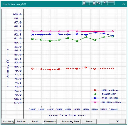
Accuracy: Accuracy is the most natural measure and is the radio of correctly predicted observations to its total observations.
Table.1 Percentage of Accuracy
Recs HAUI-Miner EHAUPMBD TUB-HAUPM MRTUB-HAUPM
100K 79.63 90.75 92.40 93.67
200K 79.49 90.47 92.38 93.73
300K 79.35 90.06 92.56 93.67
400K 79.44 90.46 92.57 93.68
500K 79.69 91.09 92.44 93.71
600K 79.62 89.96 92.70 93.73
700K 80.10 91.54 92.42 93.62
800K 79.57 90.38 93.23 93.58
900K 79.74 91.54 92.80 93.64
1000K 79.74 91.69 91.98 93.72
The above table shows the calculated percentage of accuracy. The proposed algorithm (MRTUB-HAUPM) achieved 93.72% of accuracy. Other methods like HAUI-Miner, EHAUPMBD, and TUB-HAUPM achieved 79.74%, 91.69%, and 91.98% respectively.
Figure .1 Graph Representation of accuracy rate
Accuracy comparison of different methods is shown in Figure -1.
Precision: Precision is the radio correctly predicted observations to the total observations.
Table.2 Percentage of Precision
Recs
HAUI-Miner EHAUPMBD
TUB-HAUPM
MRTUB-HAUPM
100K 79.86 91.54 92.20 94.33
200K 79.62 90.57 93.02 94.36
300K 79.31 89.55 94.19 94.24
400K 79.58 89.67 93.95 94.27
500K 79.24 90.41 93.47 94.41
600K 79.82 90.21 92.81 94.33
700K 80.08 91.40 93.23 94.24
800K 79.11 90.58 93.58 94.20
900K 79.50 91.63 92.66 94.16
1000K 79.83 91.43 92.35 94.36
HAUI-Miner, EHAUPMBD, and TUB-HAUPM achieved 79.83%, 91.43%, and 94.36% respectively.
Figure.2 Graph Representation of precision
The Figure -2 shows the comparative graph of precision for all methods.
Recall: A recall is the ratio of correctly predicted positive observations to all observations in an actual class.
Table .3 Percentage of recall
Recs HAUI-Miner EHAUPMBD TUB-HAUPM MRTUB-HAUPM
100K 79.49 90.11 92.58 93.10
200K 79.41 90.40 91.84 93.19
300K 79.37 90.47 91.22 93.18
400K 79.37 91.10 91.42 93.18
500K 79.96 91.66 91.58 93.10
600K 79.49 89.77 92.61 93.21
700K 80.11 91.67 91.74 93.09
800K 79.84 90.22 92.93 93.05
900K 79.88 91.47 92.92 93.18
1000K 79.69 91.91 91.67 93.17
The table -3 shows the calculated percentage of recall. The proposed algorithm (MRTUB-HAUPM) achieved 93.17% of recall. Other methods like HAUI-Miner, EHAUPMBD, and TUB-HAUPM achieved 79.69%, 91.91%, and 91.67% respectively.
Figure .3 Graph Representation of recall
The comparative graph for recall is shown in Figure-3 for all methods.
F-Measure: F-measure is the weighted average of Precision and Recall. Therefore, this average takes both false positives and negatives into a perspective summary. Spontaneously it is hard to understand as accuracy. In case of uneven class distribution then F1 plays a vital role and used over accuracy. Accuracy works best if false positives and false negatives have a similar cost.
Table.4 Percentage of F-Measure
Recs HAUI-Miner EHAUPMBD TUB-HAUPM MRTUB-HAUPM
100K 79.67 90.82 92.39 93.71
200K 79.52 90.48 92.43 93.77
300K 79.34 90.01 92.68 93.71
400K 79.47 90.38 92.67 93.72
500K 79.60 91.03 92.52 93.75
600K 79.66 89.99 92.71 93.77
700K 80.10 91.53 92.48 93.66
800K 79.48 90.40 93.25 93.62
900K 79.69 91.55 92.79 93.67
1000K 79.76 91.67 92.01 93.76
846
Figure.4 Graph Representation of F-Measure
This Figure – 4 shows the comparative of the F-Measure for all methods.
Processing Time: Processing time is the most important parameter in data mining. It is calculated in milliseconds (MS).
Table.5 Processing Time in ms
Recs
HAUI-Miner EHAUPMBD TUB-HAUPM
MRTUB-HAUPM 100K 17979 15496 14728 13111
200K 35971 30355 29797 26047
300K 54081 45464 44404 39001
400K 71747 60678 59282 52097
500K 89723 75761 73829 64768
600K 107677 90971 88651 77925
700K 125305 106150 103450 90450
800K 143236 121315 117775 103435
900K 161241 136678 132488 116555
1000K 179194 151815 147393 129536
The processing time for the proposed algorithm is 129536 ms other methods like HAUI-Miner, EHAUPMBD, and TUB-HAUPM achieved 179194, 151815, and 147393 respectively
Figure.5 Graph Representation of Processing Time
This comparison of processing time for all the models is shown in Figure – 5.
Power Consumption: The power consumption is calculated and shown in Table–6.
Table.6 Power consumption in MW
Recs
HAUI-Miner EHAUPMBD TUB-HAUPM
MRTUB-HAUPM
100K 146 132 128 82
200K 286 233 213 169
300K 432 363 297 247
400K 542 465 408 335
500K 670 571 494 399
600K 812 668 608 499
700K 969 802 710 547
800K 1090 887 807 644
900K 1220 1023 913 733
1000K 1366 1115 985 790
Figure.6 Graph Representation of power consumption
The comparative graph of power consumption is shown in Figure-6.
6. EXPERIMENTAL
SETUP
In this section, the performance of the proposed MRTUB-HAUPM algorithm is analyzed using RSD data sets. Accuracy, Precession, Recall, F-Measure, Processing time, and power consumption are measured using RSD data sets. Comparative analysis existing HAUI-Miner, EHAUPMBD, and TUB-HAUPM are taken. VC++ programming language is used to implement the proposed algorithm.
7. CONCLUSION
In this paper RSD bench mark data sets are used and the performance of the algorithm is analyzed using the various data size from 100 KB to 1000 KB. The various parameters like accuracy, precision, recall etc are estimated. The proposed algorithm performs well when compared to HAUI-Miner, EHAUPMBD, and TUB-HAUPM.
REFERENCE
[1] Agrawal.R and R. rikant, ―Fast algorithms for mining association rules,'' in Proc. Int. Conf. Very Large Data Bases, vol. 1215.1994, pp. 487_499. [2] S.-J. Yen and Y.-S. Lee, ``Mining high utility
quantitative association rules,'' in Proc. Int. Conf. Data Warehousing Knowl.Discovery, 2007, pp.283_292.
[3] Nanthini.R, Dr.N. uguna ― hrewd Technique for Mining High Utility Itemset via TKU and TKO Algorithm‖International Journal of Computer Science and Information Technologies, Vol.6(6), 2015, 5261-5264.
[4] Krishnamoorthy S. Pruning strategies for mining high utility itemsets. Expert Systems with Applications. 2015; 42(5):2371-81.
[5] Maya Joshi, Mansi Patel "A Survey on High Utility Itemset Mining Using Transaction Databases‖ International Journal of Computer Science and Information Technologies, Vol.5(6),2014, 7407-7410
[6] Jerry Chun-Wei Lin, Ting Li, Philippe Fournier- Viger, Tzung-Pei Hong, Justin Zhan, Miroslav Voznak ―An efficient algorithm to mine high average-utility itemsets‖ Elsevier 2 16, pp.233-243.
[7] P. Fournier-Viger, J. C.-W. Lin, R. U. Kiran, Y.S. Koh, and R. Thomas, ``A survey of sequential pattern mining,'' Data Sci. Pattern Recognit., vol.1, no. 1, pp. 54_77, 2017.
[8] AnitaBai, Parag S, Deshpande, and Meera Dhabu‖ elective Database Projections Based Approach for Mining High-Utility Itemsets‖ IEEE, Vol.6, March 28, 2018.
[9] Jimmy Ming-Tai Wu, Jerry Chun-Wei Lin, MatinPirouz, and Philippe Fournier-Viger, ―TUB-HAUPM: Tighter Upper Bound for Mining High Average-Utility Patterns‖ IEEE Vol.6, April 23, 2018.
[10]Vasumathi.R, Dr. .Murugan ―Efficient High Average-Utility Pattern Mining for Big Data‖ International Journal of Scientific & Technology Research, Vol.8, Issue 9, September 2019.