Compensated-Tracking-Errors-Based Adaptive Fuzzy Controller Design for Uncertain Nonlinear System with Minimal Parameterization

Compensated-Tracking-Errors-Based Adaptive

Fuzzy Controller Design for Uncertain Nonlinear

System with Minimal Parameterization

Junsheng Ren and Xianku Zhang

Laboratory of Marine Simulation and Control, Dalian, China Email: {jsren, zhangxk}@dlmu.edu.cn

Abstract—This paper addresses an adaptive fuzzy controller

design for a class of nonlinear system. The nonlinear system is in the framework of strict-feedback form. The system funtions are unknown, and external disturbances meet the triangular bound assumption. Takagi-Sugeno (T-S) type fuzzy logic systems are used to approximate the uncertain nonlinear functions. The control objective is to steering the system’s output to track a given signal. The closed-loop control system is proven to be uniformly ultimately bounded, and the tracking error converge to a neighborhood of zero through choosing appropriate parameters. Compensated tracking errors, not tracking errors, are employed to construct the controller, such that the proposed design avoids the repeated differential of virtual control law completely. Furthermore, the adaptive law is in the sense of minimal parameterization. Namely, the number of adaptive law is equal to the order of the nonlinear system. The simulation results show the effectiveness and usage of the proposed strategy.

Index Terms—adaptive control, backstepping control, fuzzy

system, tracking error, uncertain nonlinear system

I. INTRODUCTION

In recent years, adaptive control for uncertain nonlinear systems has received much attention, and many significant developments were achieved [1-2]. As a breakthrough in nonlinear control, adaptive backsteping control approach was introduced to achieve global stability [2]. Backstepping is a powerful tool for the controller design for nonlinear systems in or transformable to the parameter strict-feedback form, where _x∈ℜn _{is the state, u}∈ℜ _{is the control input, and}

p

θ∈ℜ is an unknown constant vector. The adaptive backstepping approach utilizes stabilizing functions αi and tuning functions τ_i for i=1, ," n. Calculation of these quantities require the partial derivatives ∂αi−1 ∂xj and ∂α_i−1 ∂θl .

However, these schemes can only suitable for the

systems with known dynamic models, or with the unknown parameters appearing linearly with respect to known nonlinear functions. Furthermore, conventional adaptive control methodology cannot incorporate human operators’ experiences, which are in the form of linguistic descriptions. Fortunately, fuzzy logic can use not only the sensor’s digital data, but also the operator’s language information. Hence, fuzzy systems can be applied to those systems which are ill-defined or too complex to have a mathematical model.

Therefore, analytical studies of nonlinear control, using fuzzy logic system [3], have become the popular tool to tackle the uncertainties in a dynamical system (see [4-8] and references therein). The adaptive fuzzy controller design [6] is proposed for a class of affine-type nonlinear system. Controller with H_∞ tracking performance was studied in [9] for canonical strict-feedback system. The authors in [11] gave the adaptive backsteping design when not all the states are available. However, the backstepping approach brings out the problem of “explosion of terms” in [9]-[12]. This problem is caused by the repeated differentiations of virtual input. This problem also appears in the other designs which use other kinds of approximator to construct the unknown system dynamics, such as wavelet [13] and neural networks [14]. To overcome the problem of explosion of complexity inherent in adaptive fuzzy backstepping design, the authors in [15] proposed a command filter backstepping (CFB) control design method. The methodology therein is useful for the system with exactly known dynamics.

Motivated by the aforementioned observations, in this paper, compensated-tracking-error-based adaptive fuzzy backstepping control approach is proposed for a class of strict-feedback nonlinear system. The system dynamics are completely unknown. Takagi-Sugeno (T-S) fuzzy logic systems are used to model the unknown nonlinear system functions. The boundedness of all the signals in the closed-loop system is guaranteed. Compensated tracking errors are used to formulate the adaptive fuzzy controller. The proposed design avoids the repeated differential of virtual control law efficiently. Hence, the proposed controller is of simple structure. Furthermore, compared to the approach in [8], the adaptive law is in the sense of minimal parameterization. That is, the Manuscript received December 8, 2012; revised April 13, 2013;

accepted July 1, 2013.

number of adaptive law is equal to the order of the system. Finally, simulation researches are carried out.

II.PROBLEM STATEMENT AND PRELIMINARIES This section will present some descriptions of problem formulations and some useful preliminaries.

A. Problem Statement

Consider a class of n-th order single-input-single-output nonlinear system in strict-feedback form as follows

1 2 1 1

2 3 1 2 2

1 1 1 1 1

1

( ) , ( , ) ,

( , , ) ,

( , , ) ,1 ,

n n n n n

n n n n

x x f x d x x f x x d

x x f x x d

x u f x x d i n

− − − −

= + +

⎧

⎪ = + +

⎪⎪ ⎨

⎪ _{= + +}

⎪

= + + ≤ ≤

⎪⎩

"

"

"

(1)

where x=[ ,x1",xn]∈ℜnis the state vector with initial condition x(0)=x₀, the first state x1 is considered as the

scalar output, and u is the scalar control signal. The functions ( , , ) :₁ i

i i

f x " x ℜ → ℜ are assumed to be unknown and satisfy the following assumption. External disturbances d_i are unknown smooth functions that satisfy the following growth conditions.

Assumption 1 (Triangular bounds): There exist (not necessarily known) parameter values * ₀

i

ψ ≥ and smooth functions p x_i( , , )₁" x_i , such that for all

n

x∈ℜ andt∈ℜ+,

* 1

( , ) ( , ),1 1.

i x t φi p xi xi i n

Δ ≤ " ≤ ≤ − (2)

Our objective is trajectory tracking. Therefore, we assume there is a desired trajectory x_1c( ) :t ℜ → ℜ+ . Specific assumptions related to this desired trajectory will be stated in subsequent sections. The objective of the control design are to specify a control signal u t( ) to steer

( )

x t from any initial conditions to track the reference input x1c( )t , to achieve boundedness of all signals and states defined in the control law, and to achieve boundedness for the system states x ti( ) from i=2, , ." n B. Useful Lemmas

To proceed, the following simple lemmas play an important role in the manipulations of our main results on adaptive fuzzy controller design.

Lemma 1 (Young’s inequality): [10] For scalar time functions x t( )∈ℜ and y t( )∈ℜ, it holds that

2 2

1 2xy x ωy

ω

≤ + (3)

for any ω>0.

Lemma 4 IF there exists

2

AB u

A B ε

=

+ (4)

where u is control input, ,A B≠0, ,A B∈ℜ, and ε>0, then Au+ A B≤ε will always holds.

Proof: Substitute (4) into the left side of the inequality, and we have

2

A B A B Au A B

A B A B

ε ε ε

ε

ε ε

+

+ ≤ ≤ ≤

+ + (5)

C. Descriptions of T-S Fuzzy System

Generally, fuzzy logic system consists of four parts: the knowledge base, the fuzzifier, the fuzzy inference engine, and the defuzzifier. The knowledge base contain a group of IF-THEN rules. Especially, T-S fuzzy rules [16] are a set of linguistic statements in the following form

j

R : IF x1is 1

j

F and x₂is F₂jand "and x_n is F_nj, THEN yj =a0j+a x1 1j + +" a xnj n,j=1, 2, , ," K where x_i are the input variables, ,a i_ij =0,1, ," n are the unknown constants to be adapted, yj is the output variable of the fuzzy system, and j

i

F are fuzzy sets associated with membership functions j( )

i i F x

μ . Together with singleton fuzzifier and center-average defuzzifier, and product inference, the crisp output of T-S fuzzy system can be expressed as follows

1 1

1 1 1

( )

( ) ( ) ,

( ) i

j

K n

j

j F i _K

j i

j j K n

j j

F i j i

y x

y x x y

x μ

ζ μ

= =

= = =

⎡ ⎤

⎢ ⎥

⎣ ⎦

= =

⎡ ⎤

⎢ ⎥

⎣ ⎦

∑ ∏

∑

∑ ∏

(6)

where

0 1 1

j j j

j n n

y =a +a x +"a x , (7)

1 1 1

( ) ( )

( ) i

i n

i F i i

j K n

j F i j i

x x

x μ ζ

μ

= = =

=

⎡ ⎤

⎢ ⎥

⎣ ⎦

∏

∑ ∏

, (8)

which is called fuzzy basis function. From universal approximation theorem [16], it is well known that T-S fuzzy logic system (6) is capable of uniformly approximating any well-defined nonlinear function over a compact set Uc to any degree of accuracy with triangular or Gaussian membership function. Due to their approximation capability, we can assume that the nonlinear system in (1) can be approximated by the above T-S fuzzy logic systems. Next, similar to the process in [16], (6) can be easily written as

0 1

( ) ( ) z ( ) z

[

1 2

]

( )x ( ), ( ),x x K( )x

ζ = ζ ζ "ζ ,

[

]

T

1, , ,2 n X = x x " x ,

T 0 1 2

0, , ,0 0

K z

A = ⎣⎡a a "a ⎤_⎦ ,

1 1 1

1 2

2 2 2

1 1 2

1 2

n n z

K K K

n

a a a

a a a

A

a a a

⎡ ⎤

⎢ ⎥

⎢ ⎥

=

⎢ ⎥

⎢ ⎥

⎣ ⎦

" "

# # % #

" .

III. ADAPTIVE FUZZY CONTROLLER DESIGN BASED ON COMPENSATED TRACKING ERROR

In this section, we will incorporate backstepping method into the adaptive fuzzy control design for nth

-order system, which is described by the equation (1). The detailed design procedure is described in the following steps.

Step 1: Firstly, we define two tracking errors for the statex₁respectively as follows

1 1 1c

x = −x x , (10)

1 1 1

x = −x ζ , (11)

where x₁c is the desired trajectory, x1is tracking error,

and x1 is compensated tracking error. Because f x1( )1 is

an unknown continuous function, we will construct T-S fuzzy system with input vector x1to approximate the

system function f x₁( )₁ . Then, similar to section II-C,

1( )1

f x can be expressed as

(

)

1 1 1 1 1 1

0 1

1 1 1 1 1 1 1 1

1 0 1

1 1 1 1 1 1 1 1 1 1

1 1 1 1 1

( ) ( )

( ) ( ) ( ) ( ) ( ) ,

z

z z

z z z c

z

f x x A

x A x A x

x A x x A A x

x A

ζ δ

ζ ζ δ

ζ ζ

ζ ξ δ

= +

= + +

= + +

+ +

(12)

where 0 1

1, 1, 1

z z z

A A A are matrices with unknown elements,

1

ξ will be defined later. Then, we obtain

1 1 2 1( )1 z1 1 1,

x =x +ζ x A x + Ω (13)

where Ω1 is an introduced variable for simplicity and

will be discussed as follows

0 1 1

1 1 1 1 1 1 1 1 1 1 1 *

1 1 1 1

0 1 1

1 1 1 1 1 1 1 1 1

*

1 1 1 1 1

1 1 1

( )( ) ( )

( )

( ) ( )

( )

( ),

z z c z

c

z z c z

c

x A A x x A

p x x

x A A x x A

p x x

x

ζ ζ ξ δ

φ

ζ ζ ξ

δ ψ

ϑψ

Ω = + + +

+ −

≤ + +

+ + +

≤

(14)

where cϑ1 is a constant only for analytic purpose, the

accurate value of which is not necessarily known, * 1

δ is the bound of approximation error, and

{

0 * *

}

1 1 1 1 1 1 1 1

1 1 1 1 1 1 1 1 1

max , , , ,

( ) 1 ( ) ( ) + ( ) ,

c c

A c x c x p

x x x x

ϑ ϑ

ϑ δ

ψ ζ φ ζ ξ

= + ⋅ +

= + + ⋅

(15)

where • stands for Euclidean norm of vectors and induced norm of matrices. Next, we define

0 1 k1 1 (x2c x2c)

ξ = − ξ + − , (16)

0

2c 1 2

x =α ξ− , (17)

where ξ₂ will be define in Step 2, the signal 0 2c x is filtered to produce the command signal x2c and its derivativex_2c, α₁ is virtual control input which will be discussed later, k1 is a positive constant and chosen by

designer. Such a filter will be defined later. By use of (16) and (17), the dynamics of the compensated tracking errors are described by

1 1 1

x =x −ξ =ζ₁( )x A x_{1 1 1}1 + Ω +₁ x₂+α₁+k_{1 1}ξ. (18) Choose Lyapunov candidate function as follows

2 1 2

1 1 1 1

1 1 _,

2 2

V = x + Γ−ς (19)

where *

1 1 ˆ1

ς =ς −ς , and Γ₁ are positive constant, which will be chosen by designer. Note that, we use compensated tracking error, not tracking error in the conventional schemes, to formulate Lyapunov candidate function in our design. Essentially, we use compensated tracking errors to remove the repeated differentiation of virtual control laws. Then, the derivative of the Lyapunov candidate is given as follows.

1 1

1= 1 ( )1 1 1 1 1 1 2 1 1 1 1 1 1 1 1

V x ζ x A x + Ω +x x x +xα +x kξ + Γ−ς ς (20) We discuss some items in the above formulae. From Young’s inequality in Lemma 1, we have

( ) ( )

1

1 1 1 1 1 1 1

2 ₂

2 T T *

1 1

1 1 1 1 1 1 1 1 1 1 1 1

( )

( )

2 2

m

x x A x x

c w

x x x A x x x x

w

θ ζ

ζ ζ χ ψ

+ Ω

≤ + +

* 2 T * 1 T

1 1 1 1 1 1 1 1 1 1 2 2 1

2 T *

1 1 1 1 1 1 1 1 1 1 1

2 T 1 T

1 1 1 1 1 1 1 1 1 1

1

1 _{( ) ( ) ( )}

2 2

1

ˆ ( ) ( ) ˆ ( )

2

1 _{( ) ( ) ( )}

2 2

w

x x x x x x x

w

x x x x x

w

w

x x x x x x x

w

ς ζ ζ ς ψ

ς ζ ζ ς ψ

ς ζ ζ ς ψ

≤ + +

≤ +

+ + +

(21)

We use the following virtual control law

2 2

T 1 1 1

1 1 1 1 1 1 1 1 1

1 1 1

1 1

1 1

( ) ( ˆ ˆ 1 _{ˆ ( ) ( )}

ˆ )

2 k x

w x x x x x

x ς ϑ ψ

α ς ζ ζ

ς ψ ε

= − − −

+

with adaptive law

2 T

1 1 1 1 1 1 1 1 1 1

1 0 1 1 1

1

ˆ ( ) ( ) ( )

2 ˆ ( )

x x x x x

w

ς ζ ζ ψ

σ ς ς

⎡

= Γ _⎢ +

⎣

⎤

− − _⎦

(23)

where σ₁≥0 , ε₁≥0 , 0 1

ς are design constants. Furthermore, by completing squares, there exists the following inequality

(

₀

)

₂

(

₀

)

2

(

_{* 0}

)

2

1 1 1 1 1 1 1 1

1 1 1

ˆ ˆ

2 2 2

ς ς ς − ≤ − ς − ς ς− + ς −ς (24)

Then, substituting (21)-(23) into (18) yields

1

2 1 2 1 2 1 * 0

1 1 1 ₂ 1 ₂ 1 + ₂ ( 1 1) 1 2

w

V ≤ −k x + x −σ ς σ ς −ς + +ε x x (25) We introduce

{

}

1: min 2 1 1, 1 1 ,

c = k −w σΓ ₁: 1

(

₁* ₁0

)

2 ₁, 2

σ

ϖ = ς −ς +ε (26)

then V can be further written as follows

(

)

1 1 1 1, 1 1 1 2.

V ≤ −c V x ς +ϖ +x x (27) Step i (2≤ ≤ −i n 1): Similar to Step 1, we define two

tracking errors for the state xi respectively as follows ,

i i ic

x = −x x (28)

, i i i

x = −x ξ (29)

where x_ic is the desired trajectory, x_i is tracking error, and xi is compensated tracking error. Then we use T-S fuzzy system to approximate unknown function f xi( )i . The dynamics of tracking errors can be expressed as follows

1

1 .

i i i i i i

x =x₊ +ζ A x + Ω (30)

Next, we define

0 ( 1) ( 1)

( ),

i ki i xi c xi c

ξ = − ξ + ₊ − ₊ (31)

0

( 1)i c i ( 1)i ,

x ₊ =α ξ− ₊ (32)

where the signal 0 ( 1)i c

x ₊ is filtered to produce the command signal x_{( 1)i+ c} and its derivative x_{( 1)i+ c}, α_i is virtual control input which will be discussed later, ki is a positive constant and chosen by designer. Then we obtain

1 .

i m

i i i i i i i i i

x =ζ c A xϑ + Ω +x+ +α +kξ (33) Choose Lyapunov candidate function

2 1 2

1

1 1 _,

2 2

i i i i i

V =V₋ + x + Γ−ς (34)

where * _ˆ

i i i

ς =ς −ς , Γi is positive constant and chosen by designer. The derivative of V_i is given as follows

1

1 1

1 _ˆ

.

i i i i i i i i i i i i i i i i i i

V V xζ A x x x x xα x kξ

ς ς

− +

−

= + + Ω + + +

+ Γ

(35)

We use the following virtual control law

1 2 2

1 _{ˆ ( ) ( )}

( ) ( 2 ˆ

)

,

ˆ i i

T i i i i i i i i i i

i i i i i i i k x

x x

x x x x

w x

α ζ

ς ψ ε ς ζ

ς ψ

−

− −

−

+

= −

(36)

where

( )

( )

( )

( ) 1 ,

i xi i xi i xi i xi i

ψ = + ζ + φ + ζ ⋅ξ (37)

( ) ( )

( )

(

)

1

1

2 0

1 ˆ

2 ˆ

.

T

i i i i i i i i i i

i

i i i

x x x x x

w

ς ζ ζ ψ

σ ς ς

⎡

= Γ _⎢ +

⎣

⎤

− − _⎦

(38)

From (36)-(38), we obtain

(

,

)

1,

i i i i i i i i

V = −c V x ς +ϖ +x x₊ (39) where

{

1

}

: min 2 , ,2 ,

i i i i i i

c = k −w σΓ c₋ (40)

(

)

1 ₂

* 0 1

: ,

2 i

i

i s i i i

s

σ

ϖ −ϖ ς ς ε

=

=

∑

+ − + (41)

Step n: We define two tracking errors for the state xn respectively as follows

, n n nc

x =x −x (42)

,

n n n

x =x −ξ (43)

The unknown function fn

( )

xn is approximated by T-S fuzzy system. Then, we obtain

( )

1 _.

n n n n n n n

x= +u ζ x A x + Ω +kξ (44)

Next, we define

,

n n n

x =x −ξ (45)

(

0

)

_.

n kn n uc uc

ξ = − ξ + − ₍₄₆₎

Furthermore, note that 0 _.

c c

u =u =u Then, we obtain .

m

n n n n n n

x= +u ζ c A x_ϑ + Ω +kξ (47) Choose Lyapunov candidate function

2 1 2

1

1 1 _,

2 2

n n n n n

V =V₋ + x + Γ−ς (48)

where * _ˆ

n n n

ς =ς −ς , Γn is positive constant and chosen by designer. The derivative of Vn is given as follows

1 1

1 ˆ .

n n n n n n n n n n n n n n n

We use the following control law

( ) ( )

T 1 2 2 1 _ˆ 2 ˆ ( ) ( , ˆ )

n n n n n n n n n

n n n n n n n n n

u k x x x x x

w x x x ς ζ ζ ς ψ ς ψ ε − = − − − + − (50) where

( )

( )

( )

( ) 1 ,

n xn n xn n xn n xn n

ψ = + ζ + φ + ζ ⋅ξ (51)

( ) ( )

( )

(

)

2 T 0 1 ˆ 2 ˆ

n n n n n n n n n n

n

n n n

x x x x x

w ς ζ ζ ψ σ ς ς ⎡ = Γ _⎢ + ⎣ ⎤ − − _⎦ (52) We introduce

{

1

}

: min 2 n n, n n,2 n

C = k −w σ Γ c₋ (53)

(

)

1 ₂ * 0 1 : , 2 n n

i n n n

i

M ϖ σ ς ς ε

− =

=

∑

+ − + (54)

then, Vn will be rewritten into

(

,ˆ

)

.

n n n n

V ≤ −CV x ς +M (55)

The above equation (61) implies that

( )

( )

( )

( )

0 0 0 0 e , .

C t t

n n

n

C V t V t

M C

V t t t

M

− −

≤ +

≤ + ∀ ≥

(56)

As a result, all xi and ςi belong to the compact set

(

i, i

) ( )

n n

( )

0 .

M

x V t V t

C ς

⎧ _{≤ +} ⎫

⎨ ⎬

⎩ ⎭ Namely, all the signals, i.e.

i

x and ςi in the closed-loop system are bounded. From (31), it is concluded that _{( ) ( )}0

1 1

i c i c

x ₊ −x ₊ can be made arbitrarily small by well-defined command filter. Then, compensated tracking error ξi is bounded. When

( )i1c ( )0i1c

x ₊ −x ₊ approaches zero, then ξ →i 0 and i i

x →x .Therefore, x_i is bounded, since x_i is bounded. Namely, the tracking errors xi are UUB. Furthermore, appropriate choice of design parameters will make the ultimate error bound arbitrarily small.

IV.SIMULATION EXAMPLE

To illustrate the fuzzy adaptive control procedures, we consider the second-order nonlinear system

( )

( )

( )

( )

( )

( )

( )

( )

(

)

1

0.5

1 2 1 2 1 1

2

2 1 2 1 1 2

e ,

sin , ,

x

x t x t x x t f x x t u t x x u t f x x

− ⎧ = + = + ⎪ ⎨ = + = + ⎪⎩ (57)

where f₁

( )

x₁ and f₁

(

x x₁, ₂

)

are unknown nonlinear functions. The control objective is to guarantee that all

the signals in the closed-loop system are bounded, and the output follows reference signal x₁c=sin

( )

t 2 . Choose membership functions of x t1

( )

and x2

( )

t as

follows

( )

(

)

1 2 1 1 3

exp , 1,2, ,5

16 l F x l x l μ = ⎡⎢− − + ⎤⎥ = ⎢ ⎥ ⎣ ⎦

" (58)

( )

(

)

2 2 2 2 3

exp , 1,2, ,5

16 l F x l x l μ = ⎡⎢− − + ⎤⎥ = ⎢ ⎥ ⎣ ⎦

" (59)

where the membership functions of x t1

( )

andx2

( )

t are

of the same structures, l denotes the number of membership functions. In this example, we use totally 5 rules to construct T-S fuzzy system for the unknown parts, namely, f1

( )

x1 and f1

(

x x1, 2

)

.

From the membership functions of x t₁

( )

andx₂

( )

t , we define the fuzzy basis functions for unknown nonlinear functions f₁

( )

x₁ and f₁

(

x x₁, ₂

)

as follows

(

)

(

)

2 1

1 ₅ 2

1 1 3 exp 16 3 exp 16 j n x j x n ζ = ⎡ _{− +} ⎤ − ⎢ ⎥ ⎢ ⎥ ⎣ ⎦ = ⎡ _{− +} ⎤ − ⎢ ⎥ ⎢ ⎥ ⎣ ⎦

∑

(60)

(

)

(

)

(

)

(

)

2 2 1 2

2 _{2 2}

5 1 2 1 3 3 exp exp 16 16 3 3 exp exp 16 16 j n

x j x j

x n x n

ζ = ⎡ − + ⎤ ⎡ − + ⎤ − − ⎢ ⎥ ⎢ ⎥ ⎢ ⎥ ⎢ ⎥ ⎣ ⎦ ⎣ ⎦ = ⎧ ⎡ − + ⎤ ⎡ − + ⎤⎫ ⎪ _{− −} ⎪ ⎢ ⎥ ⎢ ⎥ ⎨ ⎬ ⎢ ⎥ ⎢ ⎥ ⎪ ⎣ ⎦ ⎣ ⎦⎪ ⎩ ⎭

∑

(61)

where j=1,2, ,5." We use the virtual control law

( ) ( )

1

1 1 1 1 1 1 1 1 1

2 2 1 1 1 1 1 1

1 ˆ 15

20 ˆ

( )

( ) 0.5, ˆ

T

x x

x

x x x x

x α λ ζ ζ ς ψ ς ψ = − + − − (62)

with parameter adaptation laws

( ) ( )

( )

(

)

2

1 1 1 1 1 1 1 1 1

1

1 ˆ 5

20 ˆ

0.1 0.01 , T

x x x x x

ς ζ ζ ψ ς ⎡ = + ⎢⎣ − − _⎤⎦ (63)

and the following control law

( ) ( )

2 2 2 2 2 2 2 1

2 2 2 2 2 2 2 2

2 2 1 ˆ 10 2 ˆ ( )

( ) 0 5. , ˆ

T n

u x x x x x x

w x x x λ ζ ζ ς ψ ς ψ = − − + − − (64)

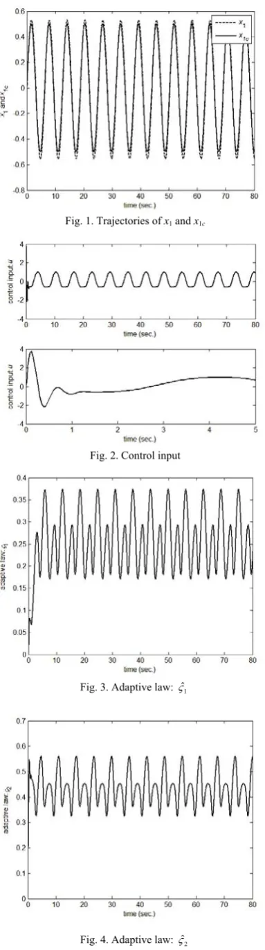
Fig. 1. Trajectories of x1 and x1c

Fig. 2. Control input

Fig. 3. Adaptive law: ςˆ1

Fig. 4. Adaptive law: ςˆ₂

( ) ( )

( )

(

)

2

2 2 2 2 2 2 2 2 2

2

1 ˆ 5

2 ˆ

0.1 0.02 . T

x x x x x

ς ζ ζ ψ

ς

⎡

= _⎢⎣ +

− − _⎤⎦

(65)

We use the following command filter

0

2 2

20

( ) ( ) .

20

c c

x t x t

s⎡ ⎤

= _{⎣ ⎦}

+ (66)

Simulation results in Fig. 1-4 show the effectiveness of the proposed adaptive control design. Fig. 1 shows that the tracking error converges to a small neighborhood around zero. Fig. 2 shows that the boundness of control input. The enlarged part, namely, the time response of the beginning5 seconds, shows that the control input is quite smooth without heavy chattering. Fig. 3-4 show the time histories of adaptive parameters ςˆ1 and ςˆ2 .From the

figures, it can be concluded that all the signals in the closed-loop is UUB.

V.CONCLUSIONS

In this paper, adaptive tracking fuzzy control scheme is proposed for a class of nonlinear system in strict-feedback form. The system dynamics are completely unknown, and external disturbances satisfy triangular bounds. The proposed algorithm can guarantee the boundedness of all the signals in the closed-loop system. Compensated tracking errors, not tracking errors, are used to construct the controller. The proposed design avoids the repeated differential of virtual control law completely, which make the controller structure quite simple and easy to implement. Furthermore, the adaptive law achieves minimal parameterization. Numerical example is used to demonstrate the effectiveness of the control algorithm.

ACKNOWLEDGMENT

This work is supported in part by National Natural Science Foundation of China under Grant No. 51109020 & 50979009, National 973 Projects of China under Grant No. 2009CB320800, and the Fundamental Research Funds for the Central Universities No. 2011JC022.

REFERENCES

[1] P. A. Ioannou, J. Sun, Robust Adaptive Control. Prentice

Hall, 1995.

[2] M. Krstić, I. Kanellakopoulos, and P. Kokotović,

Nonlinear and Adaptive Control Design. John Wiley & Sons, 1995.

[3] T. Takagi, and M. Sugeno, “Fuzzy Identification of

Systems and its Applications to Modelling and Control,”

IEEE Transactions on Systems, Man and Cybernetics, vol. 15, pp. 116–132, January 1985.

[4] Y. S. Yang, J. S. Ren, “Adaptive Fuzzy Robust Tracking Controller Design via Small Gain Approach and its Application,” IEEE Transactions on Fuzzy Systems, vol. 11,

pp. 783–795, November 2003.

[5] J. Ren, X, Zhang, “Adaptive Fuzzy Controller Design for Strict-Feedback Nonlinear System Using Compensated

Systems and Knowledge Discovery (FSKD), July 2011,

Shanghai, China, pp. 489–493.

[6] J. Ren, X, Zhang, Fuzzy-Approximator-Based Adaptive Tracking Controller Design for a Class of Nonlinear System, International Conference on Intelligent Control and Information Processing (ICICIP), August 2010,

Dalian, China, pp. 160–164.

[7] F. C. Teng, A. Lotfi, and A. C. Tsoi, “Novel Fuzzy Logic Controllers with Self-Tuning Capability,” Journal of Computers, vol. 3, 9–16, November 2008.

[8] Y. Wu, M. Zhu, Z. Zuo, and Z. Zheng, “Adaptive

Trajectory Tracking Control of a High Altitude Unmanned

Airship,” Journal of Computers, vol. 7, 2781–2787,

November 2012.

[9] W. Y. Wang, M. L. Chan, T. T. Lee, and C.H. Liu,

“Adaptive Fuzzy Control for Strict-Feedback Canonical Nonlinear Systems with H∞Tracking Performance,” IEEE Transactions on Systems, Man and Cybernetics, vol. 30, pp. 878–885, November 2000.

[10]J.T. Spooner, M. Maggiore, R. Ordonez, and K.M. Passino,

Stable Adapitve Control and Estimation for Nonlinear Systems: Neural and Fuzzy Approximator Techniques. John Wiley & Sons, 2002.

[11]W. Chen, and Z. Zhang, “Globally Stable Adaptive

Backstepping Fuzzy Control for Output-Feedback Systems

with Unknown High-Frequency Gain Sign,” Fuzzy Sets

and Systems, vol. 161, pp. 821–836, 2010.

[12]S. S. Zhou, G. Feng, and C. B. Feng, “Robust Control for a Class of Uncertain Nonlinear Systems: Adaptive Fuzzy

Approach Based on Backstepping,” Fuzzy Sets and

Systems, vol. 151, pp. 1–20, 2005.

[13]C. F. Hsu, C. M. Lin, and T. T. Lee, “Wavelet Adaptive Backstepping Control for a Class of Nonlinear Systems,”

IEEE Transactions on Neural Networks, vol. 17, pp. 1175–

1183, October 2006.

[14]M. M. Polycarpou, and M. Mears, “Stable Adaptive

Tracking Of Uncertain Systems Using Nonlinearly Parameterized On-line Approximators,” International Journal of Control, vol. 70, pp. 363–384, 1998.

[15]W. Dong, and J. A. Farrell, M. M. Polycarpou, V. Djapic, and M. Sharma, “Command Filtered Adaptive

Backstepping, IEEE Transactions on Control Systems

Technology,” vol. 20, pp. 566–580, May 2012.

[16]L. X. Wang, Adaptive Fuzzy Systems and Control: Design and Stability Analysis. Prentice Hall, 1994.

Junsheng Ren is currently a professor at Dalian Maritime University, and has been lecturing on graduate course Marine Cybernetics. He achieved his PhD degree in Communication and Transportation Engineering from the same university in 2004. He has authored or coauthored more than 40 journal and conference papers in the recent years. His current research interests include ship's maneuverability prediction, machine learning and their applications in marine cybernetics.

Xianku Zhang is born in 1968 in Liaoyang county in P. R.

China. He is currently a professor in Dalian Maritime University, and achieved his PhD degree from the same university in 1998. He has published 7 books, such as Ship Motion Control, Control System Modeling and Digital Simulation, Visual Basic Engineering Applications and etc. he