Maintenance process control: cellular automata approach

(1)

Maintenance process control: cellular automata

approach

Mustapha Ouardouz

1,∗

, Abdes Samed Bernoussi

2

, Hamidou Kassogué

2

, Mina Amharref

2

1_{MMC Team, Faculty of Sciences and Techniques, BP. 416, Tangier, Morocco} 2_{GAT Team, Faculty of Sciences and Techniques, BP. 416, Tangier, Morocco}

Abstract

In this work we consider an industrial maintenance process control problem using cellular automata approach. The problem consists on finding an optimal control for the assignment and the displacement of agents in a spatial area to maintain the equipments in good working state. The approach by cellular automata is based on: an operating statistics for determining the attributes of equipments and agents as the cells states factors; an optimal displacement of agents; an assignment of agents to equipments by Voronoi diagram as a control performing in a closed loop. The global state of the model evolves then under the mutual action of an autonomous transition function with the feedback control. We have designed in Java Object Oriented Programming a simulation software for real-time monitoring of the maintenance process scenarios in 2D and 3D scenes. The simulation results are for a production section of a factory in Tangier (Morocco).

Receivedon 30 May 2016;acceptedon 09 September 2016;publishedon 06 March 2017

Keywords: Cellularautomata,Feedbackcontrol,Maintenanceprocess,Resourcesallocation,Assignment.

Copyright © 2017 Mustapha Ouardouz et al., licensed to EAI. This is an open access article distributed under the termsoftheCreativeCommonsAttributionlicense(http://creativecommons.org/licenses/by/3.0/),whichpermits unlimiteduse,distributionandreproductioninanymediumsolongastheoriginalworkisproperlycited.

doi:10.4108/eai.6-3-2017.152337

1. Introduction

From the 1980s with the development of computers, cellular automata (CA) theory has boomed in the world of science. They gradually emerged as an alternative for the microscopic realities, reflecting the macroscopic behavior of dynamic systems. They are now used as modeling tools in many sciences area. Research in biology and chemistry were the first predisposed to exploit them. Today there are lots of applications in all areas involving the variables space and time. Indeed, by the cellular automata approach, they are taken discretely, as well as the physical quantities they describe.

Since their introduction in the 1940s as a model of self-replicative systems considered by Von Neumann and Ulam, many were the definitions around the CA, [1] (1998), [2][3] (2002) and [4] (2008). But the concept was always the same: a mutual interaction between neighboring cells governed by simple local rules, which results to a complex global dynamics evolution.

∗

Corresponding author. Email:[email protected]

Their definition simplicity, as well as their adaptation to strong computer architectures with respect to continuous models justify their heavy use as modeling tools in recent decades. Most recently Ouardouz et al. in [5] have proposed an CA model for the agents allocation process in a maintenance problem in industry, to meet the needs of resource allocation under constraints of space, cost and time. The determination of the mathematical model for such phenomenon described by a distributed parameters system is the first step in the classic study of this kind of system (understanding the system, follow its evolution in the aim to control it). The cellular automata approach yet in this case present a huge advantage compared to its description relatively simple and for its adaptation to global realities of the problem considered.

Therefore, the need to define and characterize the concepts long exposed in the systems theory is required for cellular automata approach, like the concepts of controllability and spreadability [3,4].

In this paper, we consider the controllability concept for cellular automata in order to approach the maintenance process problem. For that, we consider

(2)

the model, proposed by Ouardouz et al. in [5] in the autonomous case, and we perform a feedback control to optimize the assignment displacement of agents as we introduced in the proceeding [6].

In the second section we recall some generalities on cellular automata principle and the controllability concept. In the third section, we present the problem statement. In section four we present the methodology for the problem approach and some simulations results illustrating our approach for a factory in Tangier.

2. Cellular Automata: generalities

2.1. Cellular automata definition

A cellular automata (CA) is given by a quadruplet [4]

A₍T_,V_,E_{, f}₎ ₍₁₎

where:

• T _{called cell space or lattice is a network which}

consists on a regular tiling of a domain ΩofRn, n= 1,2 or 3. The elements of this paving denoted

care said cells and occupy the whole area.

• v called neighborhood, for accell is a set of cells affecting its evolution over time. Depending on the problem modeled, it can be given by

v(c) ={_c0 ∈ T_; _d₍_{c, c}0₎≤_r}_, ∀_c∈ T_. ₍₂₎

d is a distance on T × T _{equivalent to the norm}

L∞defined by [3]

d(c, c0) = min{_`₍_{c, c}0_{); (}_{c, c}0₎∈_J₍_{c, c}0₎}_, ∀_{c, c}0∈ T

(3) where `(c, c0

) is a length between c and c0

and

J(c, c0

) the set of all possible joins betweenc and

c0

from their center.v(c) is said radiusr and size

m= cardv(c).

• E _{designates all states, which is a finite set of}

values representing all states that may be taken by each cell. This is generally a cyclic ring, given by

E ₌{_e₁_{, e}₂_{, . . . , e}_k} _{with card}E _{= k}_. ₍₄₎

We speak about a configuration of a CA in a given timet, the application

et: T → E

c 7→ _e_t₍_c₎ (5)

which maps each cellcfromT _{a value taken in}E

which will be the state ofcat timet.

• f is a transition function that defines the local dynamics of the considered system. It calculates the state et+1(c) of a cell at t+ 1 depending

on the state et(v(c)) ={et(c

0

), c0 ∈_v₍_c₎} _{of the}

neighborhood att. We consider then the form

f : Em → E

et(v(c)) 7→ et+1(c) . (6)

2.2. Controllability for cellular automata

First let’s see how we can introduce a control in a cellular automaton as outlined in [3,4]. As in the case of continuous systems, a precision on the control is to give its spatial support and distribution and its values.

• The spatial support of the control will be a part of the lattice where the control is applied, noted

T_u ⊂ T_. ₍₇₎

• The spatial distribution of the control will be a part of the lattice where the control act, noted

ω⊂ T_. ₍₈₎

• The values of the control will be provided by the set of values

U ={_u₁_{, u}₂_{, . . . u}_q}_. ₍₉₎

SomeU values can of course be in the set of statesE_{. In}

what followsIis a discrete time interval.

Definition 1. LetA₍T_,V_,E_{, f}₎_{be a cellular automaton}

and letT_u ⊂ T_{. The control over}A_{is a function}

u:T_u×_I →_U ₍₁₀₎

which to each cellcfromT_u _{associates a value}_u_t₍_c₎_in_U _at

t, which act on the state ofω. In this caseA_{becomes a}

non-autonomous or a controlled cellular automaton denoted

A_u₍₍T_,V_,E_{, f}₎_{, u}₎_.

The support of the control u in some cases may be reduced to a single cell, in this case we speak of punctual control. In other cases, the support may vary in time and space. The support may be expressed by

T_u₌_supp₍_u_{) =}[

i n

c∈ T_;_u_t₍_c_{) =}_u_i ∈_Uo_. ₍₁₁₎

Similarly with continuous systems, we may adopt a formulation of the transition function in the case of a controlled CA as

fu:Em×Um → E

(et(v(c)), ut(v(c))) 7→ et+1 (12) where ut(v(c)) ={u(c0, t)∈U;c0∈v(c)}. Acts on the control cells only in T_u_{. Another much more flexible}

formulation, which we will use for the following, is

2 _{Context-aware Systems and Applications}EAI Endorsed Transactions on

(3)

established that

fu(et(v(c))) =f(et(v(c)))⊕u(c, t)χT_u. (13)

It is clear that here the control is applied to a cellcwhen it is in the action area T_u _{of control} _u_{. The sign} ⊕ _is

interpreted as a mutual action of the control and the autonomous transition function.

Definition 2. LetA₍T_,V_,E_{, f}₎_{be a cellular automaton.}

• We say thatA_{is regionally controllable during a time}

interval]0, T[if for each initial configurationeω₀ and each desired configuratione_dωthere exists a controlu such that

eω_T =eω_d. (14)

• We say that A _{is weakly regionally controllable}

with a tolerance ε during a time interval ]0, T[ if for each initial configuration eω₀ and each desired configurationeω_d there exists a controlusuch that

card{_c∈_ω_;_e_T₍_c₎_,_e_d₍_c₎}

cardω ≤ε. (15)

For more details about controllability of cellular automata we refer to [3,4] and the references therein.

3. Maintenance process control: problem statement

The maintenance problem in industry is how to assign available technicians to a set of down equipments taking into account there proximity, availability and competencies so as to maintain as long as possible all the equipments in good working state. The starting point is a set of operational machines falling down (not necessarily all of them) after a certain uptime.

This system is a system with spatio-temporal evolution described by the states of the machines and the agents interventions over the time. It is a discrete system in time and space. Each machine and each agent occupies a geographic position at a given moment and the overall state of the system is a spatial configuration changing over time. That is why we opt for a cellular automaton approach.

It is proposed to develop a control based on the consideration of spatial and temporal factors in the allocation of resources allowing particularly, in the case of a manufacturing company to maintain all the machines operational.

We are interested in the control of the allocation of intervention tasks of preventive maintenance process for which allocation decisions and agent displacements are made by a simulation based on cellular automata.

The proposed control, must also apply in the case of unplanned interventions (random) due to corrective maintenance. Indeed, the application of

control following the observation of the distribution of resources ’technicians’ in the beggerhood of a down machine should allow to allocate maintenance tasks to the most appropriate agent, available and/or more close spatially and thus to ensure the reparation of the machine.

4. Maintenance process control: problem approach

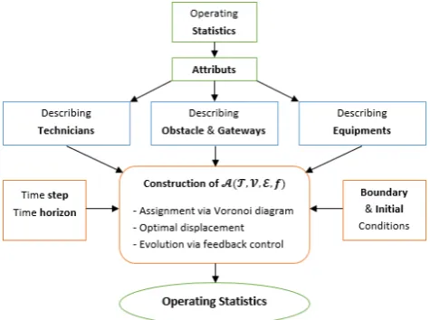
We consider the cellular automaton model as used in [5] but in this work we perform the CA model evolution under the mutual action of an autonomous transition function with a feedback control as introduced in [6]. The approach consists on determining:

• the attributes of equipments and agents as the cells states using operating statistics;

• the optimal displacement of agents taking into account the obstacles;

• an assignment of agents to equipments by Voronoi diagram as a control performing in a closed loop.

The principle of the approach by cellular automaton is illustrated in figure1.

Figure 1. Principle of maintenance process control by CA

4.1. Presentation of the CA model

Model principal. The CA Model A₍T_,V_,E_{, f}_{) for the}

studied case is constructed on a bi-dimensional lattice

T ⊂_Z2 _{where the cells in} T _noted _c_ij _{have as}

neighborhood the entire lattice

v(cij) ={ckl ∈ T;d(cij, ckl)≤cardT }=T. (16)

The set of states is given by

(4)

whose values correspond to the occupant of the cells as

et(cij) =                         

−₄ _{if an obstacle}

−₃ _{if a down equipment}

−₂ _{if an equipment under reparation} −₁ _{if an operationnal equipment}

0 if empty

1 if an available technician 2 if an occupied technician

.

(18) We denote that et(cij)<0 corresponds to a presence of an equipment in the cell or an obstacle which has fixed position, whereas a presence of a technician is indicated byet(cij)>0 which has variable position. To each equipment we associate characteristic parameters determined from previous operating statistics:

• mtbfij: the mean time between failures,

• mtbf cij: the mean time between failures counter,

• mttrij: the mean time to repair,

• mttrcij: the mean time to repair counter,

• zrij: an area of intervention which corresponds to a cell where the technician should stand up to repair the machine.

In this paper we assume that the equipment does not fail randomly, but afterMT BF. The technicians likewise have the following properties:

• ztij: a buffer zone where the technician returns at the end of the intervention.

• ccij: said target cell is the final destination of the technician.

• dij: is a couple (d1, d2)∈ {−1,0,1}2 with |d1|+

|_d₂| ≤_{1 reflecting a direction taken by the}

technician in the next moment. It is negotiated for the cell cij as a local destination ci+d1,j+d2.

d= (0,0)≡_{0 is a null direction, the technician is}

stationary. Forccijcorresponding to the index cell ckl, it is calculated as

dij =

                

(0,0) ifk=iandl=j (·₎

(1,0) if|_k−_i| ≥ |_l−_j|_and_k≥_i ₍→₎

(−₁_,₀₎ _if|_k−_i| ≥ |_l−_j|_and_k≤_i ₍←₎

(0,1) if|_k−_i| ≤ |_l−_j|_and_l ≥_j ₍↑₎

(0,−₁₎ _if|_k−_i| ≤ |_l−_j|_and_l ≤_j ₍↓₎

.

(19)

• αij: a rotation angle of{±π2,±π}performed by the technician, in case of an obstacle relative to the local direction dij. The couple [dij, αij] indicates a direction dij followed by a rotation angle αij. For example [(1,0),−π

2] = (0,1) and [(1,0),π2] = (0,−_1).

Autonomous system. The transition function f can be written firstly to define the dynamics of an autonomous system. Letet(cij) be the cellcij ∈ T state att. The cell state att+ 1 is fulfilled by

et+1(cij) =f(et(v(cij)))

=                 

−₃ _if_e_t₍_c_ij_{) =}−_{3 or if}_e_t₍_c_ij_{) =}−_{1 with}_{mtbf c}_ij_{= 0} −₂ _if_e_t₍_c_ij_{) =}−_{2 with}_mttrc_ij_>₀

−1 ifet(cij) =−1 or ifet(cij) =−2 withmttrcij= 0 1 ifet(cij) = 2 andet(ccij) =−2 withmttrccc= 0

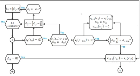
dep(cij) ifet(cij) = 1 or ifet(cij) = 2 withdij 9ccij (20) Here dep(cij) is a function that is used to implement the displacement of the technician occupying the cell

cij. In case of the intersection of several technicians, the priority to the right rule is performed. Displacement is thus made to avoid as much as possible the blockages. The diagram in figure 2 describes the displacement function where we used the following notations:

• d−₁: previous direction of the technician.

• co: obtained cell from the directiondij.

• coo: cell aftercoin the directiondij.

• cα: obtained cell from a rotation [dij, αij].

• do,doo: direction of the technician if the cellco or coocontains a technician.

Figure 2. Diagram of the technicians displacement function

dep(cij).

Controlled system: feedback control. We introduce here a feedback control on the autonomous system defined by the previous cellular automaton model. For a given time horizon T, the control will aim to keep all equipments operational. We therefore consider all down equipments

ω={_c_ij ∈ T_;_e_t₍_c_ij_{) =}−₃} ₍₂₁₎

as a spatial distribution (or region) of the control. The support of the control, will, among other be

T

4

u = {cij ∈T ; et(cij ) = 1} (22) EAI Endorsed Transactions on

Context-aware Systems and Applications

(5)

the set of available technician. We choose as the control values all

U ={₁_,₂}_. ₍₂₃₎

For a desired configurationedof the system with

ed(cij) =−1, cij ∈ω, (24)

the problem of the CA controllability we adopted is to find a controluthat achieves this configuration at the timeT. The control proposed is technicians assignment inT_u_{to down equipment in}_ω_{for maintenance, let then}

u:T_u×_I → _U

(c, t) 7→ _u₍_{c, t}₎ . (25)

A technician is assigned to an equipment when he is nearest the equipment than any one other (principle of Voronoi diagram [7]). Both are updated and removed in the assignment process and the operation is repeated until that there is no more technicians available or machines in failure. For the explicit expression of the controlu, we construct Voronoi diagrams [5] associated toTu andω:

V_or₍T_u_{) =} [

c∈T_u

RTc (26)

and

V_or₍_ω_{) =}[

c∈_ω

REc (27)

with

RTc ={c

0

∈ T_;_d₍_{c, c}0₎≤_d₍_{c, c}_”) _c_”∈ T_u}_, ₍₂₈₎

and

REc ={c

0

∈ T_;_d₍_{c, c}0₎≤_d₍_{c, c}_”) _c_”∈_ω}_. ₍₂₉₎

Then the controluis expressed by

c∈ T_u_{, u}₍_{c, t}_{) =}

(

2 if∃_c0 ∈_{ω / R}T_c ∩_RE

c0 _,∅

1 else .

(30) However, it is noted that T_u _{changes in time because}

a busy technician may become available upon control. It is the same with ω, a machine in good operating conditions could breakdown. And since the control is performed for a definite time horizon, then the control

ucan be seen in a loop farm with return on observation of the state of the system. The transition function of the controlled CA

A_u₍₍T_,V_,E_{, f}₎_{, u}₎ ₍₃₁₎

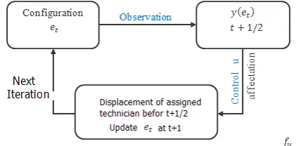
shall be defined so that all updating operations are made between the instantst,t+ 1/2 andt+ 1.

• Betweentandt+ 1/2, observations are performed on the state of the cells to notify the down equipments and available technicians (ωandT_u₎

according to the function

y:ET → T × T

et 7→ (Tu, ω) . (32)

• Betweent+ 1/2 andt+ 1, we perform the control

u(c, t+ 1/2), c∈ T_u_. ₍₃₃₎

• Att+ 1, we update the state of each cell. And all technicians can move except those engaged before

t+ 1/2.

The transition function fu of the controlled CA Au is then written

et+1(cij) = fu(et(v(cij))

= f(et(v(cij))⊕u(cij, t+ 1/2)χT_u; c_ij ∈ T

(34) where f and u are explained respectively by the equations 20 and 30 and ⊕ _{refers to the mutual}

action of the control and the autonomous transition function. The principle of closed loop control on our CA for maintenance problem is summarized in figure3. Some examples of Computer simulations after implementation of the CA are provided in the next section.

Figure 3. Principle of feedback control for maintenance process

4.2. Simulation

Simulation software. The set of algorithms for cellular automaton built above was implemented in Java Object Oriented Programming [8], using the architecture of the Model-View-Controller design pattern to define and implement all used algorithms by functionality packages. This keeps the logic and the internal representation of the model separated from the visualization and calculation management. It allows to meet the simulation needs while ensuring flexibility and re-use of source code. For real-time monitoring, we have proposed in the graphical user interface several features like:

• the construction of the lattice geometry manually or by loading an existing one;

• the load of the operating statics and then processing of the cells attributes;

(6)

• the monitoring options: speed, zoom, 2D and 3D scene;

• the output data storage, processing and export.

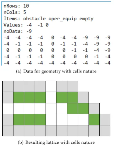
For the data management, we use an ascii file into where data are saved in raster image format. More precisely, in the two first lines we indicate the number of rows and columns, and we put in the two next lines the items and values to indicate respectively the nature of data and their corresponding values. In the fifth line we put a value which refers to no available data and finally in the successive lines we set the values along the rows and columns. An example is illustrated in the figure

4 for the construction of a lattice. The raster format

(a) Data for geometry with cells nature

(b) Resulting lattice with cells nature

Figure 4. Illustration of data syntax for lattice construction

is suitable for any lattice geometry. The same syntax can be used for attributes or any other parameters of interest.

For the output data processing, we plot the number per time step of the operational equipments, down equipments and equipements under reparation which coincides with the occupied technicians. Their average value and standard deviation are used to produce a percentage of control action for a considered simulation constraints.

Simulation case. The simulation case concerns a factory located in Tangier. It includes four production sections, each consists of a set of machines whose maintenance requires a competence. As the present model is for mono-competence (each technician can fix all reported failure), we make simulation only for one production section as illustrated in figure 5. The lattice geometry

Figure 5. The considered factory production section

describes boundary condition: fixed type for the case of walls as obstacles and reflexive type for the case of door which can contains agents. There are 3 available agents in the buffer zone and 74 machines disposed grouped in 3 types (T1, T2, T3) with particular MTBF and MTTR. For exemple, for the groupe of machines T2, the figure

6gives the operating statistics for 126 hours. From the

(a) MTBF (in min) per hour for 64 machines

(b) MTTR (in min) per hour for 64 machines

Figure 6. Operating statistic for machines T2 during 126 hours

evolution of the MTBF during the 126 hours (color blue

6 _{Context-aware Systems and Applications}EAI Endorsed Transactions on

(7)

in figure6(a)) we take its average value as the resulting MTBF (color red in figure 6(a)) for the machines T2 during the time horizon. We do the same for the MTTR in figure6(b). The table1gives the resulting MTBF and MTTR for the three machines types following the same operating statistics.

Table 1. MTBF and MTTR in min for the tree types of machines

Type MTBF MTTR

T1 300 30

T2 180 10

T3 420 45

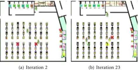
Simulation results. The considered initial condition (two down machines T2 and three available agents) is shown in figure 5 and we take randomly the initial count of the MTBF, otherwise the other machines will fall down the same time. Then, the figure 7 shows two distinct iterations obtained by time step of 30 seconds (in order to see the displacement process). For the iteration 2

(a) Iteration 2 (b) Iteration 23

Figure 7. Illustration of simulation for two distinct iterations

as shown the figure 7(a), one agent reaches the down machine while the other agent is still in displacement. 20 iterations are required to fix each machine. Then, as shown in figure 7(b), at the iteration 23 the two machines T2 are fixed, but another machine T2 fall down and the third agent is assigned to it.

Remark. In the section 4.2 of [6], we have presented more illustrative simulations evolution per time step in order to illustrate how the states of the machines and technicians change for a given time horizon. Here, we follow by presenting the statistics of the output data as explaining above.

We add then 7 additional agents and we left the system evolving for 8 hours (960 iterations of 30 seconds). Figure 8 presents the output operating statistics for all the machines. For all the states, we remark that the evolution from the simulation

Figure 8. Evolution of the number of all the machines

constraints highlights a periodic variation. Almost each 400 iterations, we have a similar variation of the number of operational equipments, down equipments and equipments under reparation which coincides with the number of occupied agents. The table2shows some indicative output operating statistics for the considered simulation.

Table 2. Output operating statistics for the considered simulation

Indicators Down Repairing Operational

minimum 0 0 61

maximum 3 10 74

average 0,28 6.86 66.86

standard deviation 0.53 2.54 2.7

The table allows us to affirm that during this simulation:

• 0 to 1.09% of machines fall down without assigned agents;

• 5.84 to 12.7% of machines are under reparation;

• 43.2 to 94% of agents are occupied for maintain;

• 86.7 to 94% of machine have good working state.

Then, the cellular automaton model is weakly control-lable with a tolerance of 14% for this simulation.

5. Conclusion and perspectives

(8)

data. The simulation results were for a production section in a factory, for which we used a simulation software we have designed in Java Object Oriented Programming. Although our model is in 2D, the simulation software take into account a 3D scene view of the lattice. But it will be very interesting to extend these results to the 3D lattice as for example the case of assignment and displacement in a building with different floors. Also it will be interesting to consider a stochastic cellular automota to model equipments falling down with multi-competences agents. Those problems are under investigation.

Acknowledgement. This work has been supported by the project PPR2-OGI-Env and the international network TDS, Academy Hassan II of Sciences and Techniques.

References

[1] B. Chopard, M. Droz(1998)Cellular automata modelling

of physical systems (Cambridge, Collection Alea-Sacley, Cambridge University Press).

[2] S. Wolfram(2002)A new king of science(Wolfram Media).

[3] A. El Jai and S. El Yacoubi (2002) Cellular automata

modeling and spreadability(Mathematical and Computer Modeling), 36:1059-1074.

[4] S. El Yacoubi (2008) A mathematical method for control

problems on cellular automata models(International Journal of Systems Sciences), 39:529-538.

[5] M. Ouardouz, M. Kharbach, A. Bel Fekih, A.

Bernoussi (2014) Maintenance process modelling with

cellular automata and Voronoi diagram (IOSR Journal of Mechanical and Civil Engineering), 3:11-18.

[6] M. Ouardouz, A. Bernoussi, H. Kassogué, M. Amharref

(2016) Maintenance process control: cellular automata approach (ICTCC 2016, LNICST), 168:287-296, DOI: 10.1007/978-3-319-46909-626.

[7] M. de Berg, M. van Kreveld, M. Overmars and O.

Schwarzkopf (2000) Voronoi Diagrams: The Post Office

Problem. Ch. 7 in Computational Geometry: Algorithms and Applications(Springer-Verlag, Berlin), 2nd rev. ed, pp. 147-163.

[8] C. Delannoy (2008) Programmer en Java (Editions

Eyrolles, Paris).

8

EAI Endorsed Transactions on

Context-aware Systems and Applications