Efficient Intelligent Localization Scheme for Distributed Wireless Sensor Networks

Efficient Intelligent Localization Scheme for

Distributed Wireless Sensor Networks

Chunlai Chai

College of Computer Science and Information Engineering, Zhejiang GongShang University, Hangzhou, China

([email protected])

Abstract—To estimate location accurately in distributed wireless sensor networks (WSNs), an efficient intelligent position estimation scheme is proposed which needs fewer known nodes without calculating relative positions. The proposed intelligent localization scheme includes two phases. In the first phase, an initialization location algorithm is adopted, where known nodes broadcast their positions and one-hop distances, and then unknown nodes use the received information and operate weighted estimation algorithm to calculate their initial positions. In the second phase, an optimized location algorithm is employed. Unknown nodes exchange information with their neighbors and operate a modified weighted estimation algorithm to refine their positions repeatedly. Additionally, a location scheme also is proposed to solve the problem that a node only has two neighbors. Detailed simulation results show that, the proposed scheme can decrease the average position error down to 9% radio range, and increase the average number of located nodes up to 78% when connectivity is greater than 12 in 20% known node ratio.

Index Terms—intelligent localization, wireless sensor networks, distributed algorithm

I. INTRODUCTION

The past few years have witnessed increased interest in the potential use of wireless sensor networks (WSN) in applications such as disaster management, combat field reconnaissance, border protection, and security surveillance [1]. In most emerging applications, each sensor node is required to report not only its sensing data but also its current position. Therefore, developing effective localization scheme has become a pressing issue in the advancement of wireless sensor networks [2, 10].

A. Related Work

The global positioning system (GPS) [3, 9] is the most widely used localization technique currently. However, fitting GPS receivers to a large number of sensor nodes is not cost-effective in most applications and it is not suitable for all sensor nodes. Although the defects of GPS are shown in previous descriptions, it remains a popular, accurate, and convenient solution for location system. Considering the advantages and disadvantages of GPS, few sensor nodes known their positions by combining

GPS is a feasible solution. Sensor nodes without GPS also can obtain their positions by location algorithm. According to the ranging technology and the limited location information, the location algorithm can determine the positions of sensor nodes.

Various mechanisms have been proposed to deal with the localization problem. From a technical perspective, these mechanisms fall into two broad categories, namely approximate positioning and exact positioning proximity [4, 12, 15]. Many approximate approaches for the determination of sensor nodes exist in literature. These approaches are often resource-efficient but also result in higher positioning errors than exact positioning approaches, especially when the input parameters have low deviation of their true value.

In [5, 13], a range-based approximate positioning approach is proposed, which is simple, has low complexity, requires a few resources, has rather good accuracy (especially in high noise situations) and is range-based. The schemes in [6, 16, 17] have more complexity, requires more resources and has lower accuracy. But, it is range-free. In contrast to approximate approaches, exact approaches use the known known node-positions and the distances to the sensor nodes in order to calculate their coordinates through the solution of non-linear equations [7, 14, 18]. Using a minimum of three known nodes (in two dimensions), the coordinates of the sensor nodes may be determined by their intersection [19, 21, 22]. The use of more than three known nodes gives more information in the system and allows the refinement of the position and the detection and removal of outlying observations. The least squares method (LSM) is used for the solution of the simultaneous equations [8, 20, 23]. The LSM produces accurate results, however it is complex and intensive and therefore it is not feasible on resource-limited sensor nodes.

B. Motivation

Although many mechanisms have been proposed to solve localization problem, there are some challenges for locating sensor nodes. The first challenge is the energy consumption problem. It is worthy to consider how to utilize the limited energy of sensor nodes to achieve position determination. The consumption origin contains activating radio frequency module when they communicate with neighbors, and activating microprocessor when they compute estimated positions.

Manuscript received January 1, 2009; revised February 15, 2009; accepted February 20, 2009.

The second challenge is the ranging error problem. This problem comes from anisotropic environment and multipath interference, and these factors lead to distance or angle measurement errors. An important note is that none of exact positioning approaches and none of approximate positioning approaches are the best in all situations and from all aspects. Some of these approaches have rather good accuracy in high noise situations and some of them have rather good accuracy in low noise situations.

In this paper, we concentrate on the localization problem in distributed wireless sensor networks where few sensor nodes known their positions by equipping with GPS. An efficient intelligent localization scheme is proposed which includes two phases: initialization phase and location estimation phase. In the initialization phase each node estimates its initial position by the proposed initialization location algorithm (ILA). In the location estimation phase, each node uses location estimation and refining algorithm (LERA) to refine position. Additionally, a location scheme also is proposed to solve the problem that a node only has two neighbors. Using a minimum of two known positions in two dimensions, the coordinates of the sensor nodes may be determined by their intersection.

The paper is organized as follows. In section 2, the proposed localization scheme is proposed in detail. Detailed simulation and analyses are shown in section 3. Finally, the conclusion and future work are given in section 4.

II. PROPOSED LOCALIZATION ALGORITHM

The proposed intelligent localization algorithm includes two phases: initialization phase and location estimation phase. In the initialization phase, sensor nodes known their positions by equipping with GPS, broadcast their position information, and then those unknown nodes can get their initial positions. In the second phase, unknown nodes only exchange information with their neighbors and then estimate their location with weighted coefficient to refine initial node positions.

A. Initialization Phase

The goal of this phase is to give the initial positions to unknown nodes. This location information will be exchanged between nodes in the second phase. The processing steps are shown in the follows algorithm 1:

Algorithm 1: Initialization Location Algorithm (ILA)

1: Nodes with GPS broadcast their positions in the network.

2: Nodes maintain the shortest paths to each other. 3: if GPS nodes received positions information then

4: compute one-hop distances;

5: broadcast these values to unknown nodes; 6: endif

7: if unknown nodes receive information then

8: estimate distances; 9: endif

10: for all unknown nodes

11: operate efficient positions estimation algorithm 12: endfor

For a node A with unknown coordinate (x_A,y_A), if

there are N known nodes nodes connected with it. From

step 1 and step 2, known nodes and unknown node A can know following information:

Real Euclidean distance between N known nodes

nodes dij, where i j, ∈[1,N]. Hop count between N

known nodes nodes h_ij, where i j, ∈[1,N]. Hop count

from A to N known nodes nodes h_Ai,i∈[1,N]

In step 3, nodes with GPS can compute their one-hop distances:

1,

1,

( ) , [1, ]

N ij j j i

i N

ij j j i

d

d B i N

h

= ≠

= ≠

=

∑

∑

one-hop (1)

In step 4, unknown node A computes average one-hop distance done-hop( )A :

1

1

( ) ( )

N

i i

d A d B

N =

=

∑

one-hop _one-hop (2)

Then unknown node A measures distance between A and N known nodes nodes dm_Ai

( ) , [1, ]

Ai Ai

dm =done-hop A h⋅ i∈ N (3)

Finally, unknown node A operates weighted optimization scheme to estimate its initial position as follows:

It calculates error between estimated distances to known nodes and measured distances to known nodes:

(

)

( ) ( ) , [1, ]

Ai A i A i Ai

f = x −x + y −y −d i∈ N (4)

To estimate (x_A,y_A) , we apply minimum square

estimation (MSE):

2

1

min

N Ai i

F f

=

=

∑

Let f_Ai=0(i∈[1,N]), then we can get the following non-linear system:

2 2 2

(xA−xi) +(yA−yi) =dAi (6)

Reduce to the linear system, we can transform to the matrix form:

,

AX=b (7)

where

1 2 1 2

1 3 1 3

1 1

2( ) 2( )

2( ) 2( )

2( N) 2( N)

x x y y

x x y y

A

x x y y

⎛ − − ⎞_⎟

⎜ _⎟

⎜ _⎟

⎜ _{− − ⎟}

⎜ ⎟

⎜ ⎟

=_{⎜ ⎟⎟}

⎜ _⎟

⎜ _⎟

⎜ ⎟

⎜ _⎟⎟

⎜ − −

⎝ ⎠

A

A

x X

y

⎛ ⎞⎟ ⎜ ⎟

=_{⎜ ⎟⎜ ⎟}

⎜⎝ ⎠ (9)

2 2 2 2 2 2

2 1 2 1 2 1

2 2 2 2 2 2

3 1 3 1 3 1

2 2 2 2 2 2

1 1 1

( ) ( )

( ) ( )

( ) ( )

A A A A

AN A N N

d d x x y y

d d x x y y

b

d d x x y y

⎛ _{− − − − −} ⎞_⎟

⎜ _⎟

⎜ _⎟

⎜ _⎟

⎜ − − − − − ⎟

⎜ _⎟⎟

=⎜_{⎜ ⎟}

⎟

⎜ ⎟

⎜ ⎟

⎜ ⎟

⎜ _⎟⎟

⎜ − − − − −

⎝ ⎠

" (10)

If the number of the equations is larger than 2, X has no solution but approximation, so this problem is equivalent to solve normal equation:

,

T T

A AX=A b (11)

Then we can get:

1

( T ) T .

X= A A−A b (12)

B. Location Estimation Phase

Based on the initialization phase, unknown nodes have got their initial positions. In this phase, nodes exchange information with their neighbors to refine their positions. When nodes receive information from at least three neighbors, they can apply certain ranging technology (e.g. RSSI) to measure distances to neighbors, and then adopts weight algorithm to estimate positions. However, positions and distances to neighbors have different accuracy. It is obviously that the position information from nodes with GPS is more accurate than that from other nodes. Similarly, according to the signal digressions properties for ranging measurement, the position information from near node is more accurate than that from far node.

Hence, we define a parameter weight w, that is the

production of neighbor's position weight and distance weight. Position weight reflects the accuracy of neighbor's position, and distance weight reflects the accuracy of ranging measurement. The steps of the location estimation phase are shown in the follows algorithm 2:

Algorithm 2: Location Estimation and Refining Algorithm (LERA)

1: Repeat

2: Unknown node calculates the weights for its neighbors. 3: Unknown node estimates its position by the weighted

optimization scheme.

4: Unknown updates its position and then floods its position weight valuew_p and position to neighbors.

5: if unknown nodes receive information then

6: estimate distances; 7: endif

8: for all unknown nodes

9: operate efficient positions estimation algorithm 10: endfor

11: Until position error converges

For location estimation and refining algorithm (LERA), an unknown node A with unknown coordinate (xA,yA), which can receive the position data from at least N

neighbors, calculates the weights for its neighbors as follows.

(a) Find the position weight wp for each neighbor,

where wp=0.1 for unknown node and wp=1 for

known node.

(b) Use ranging technology to measure distances to

each neighbor, and assign the distance weight wd

according to received power, where wd∈[0,1]. (c) Set the weight w by w=wd⋅wp.

Node A estimates its position by the weighted optimization scheme. Node A calculates error between estimated distances to neighbors and measured distances to neighbors:

2 2

( ) ( ) , [1, ]

Ai A i A i Ai

E = x −x + y −y −d i∈ N (13)

To estimate (x_A,y_A), we apply MSE to:

2

1

min

N Ai i

E f

=

=

∑

But these error functions will have the same influence

on minimizing E, this is unreasonable, so we will add

weight information:

Each neighbor's position weight is w i_ip( ∈[1,N])

respectively. Position weight of known node is always 1, and initial position weight of unknown node is 0.1.

Each neighbor's distance weight is w_id(i∈[1,N])

respectively.

Weight representing the reliability of neighbors' positions and distances to neighbors is:

, ( [1, ])

i ip id

w =w ⋅w i∈ N (15)

In step 5, the weighted error functions between estimated distances to neighbors and measured distances to neighbors:

2 2

[ ( ) ( ) ]

, ( [1, ])

i Ai ip id A i A i Ai

w f w w x x y y d

i N

= ⋅ ⋅ − + − −

∈ (16)

To estimate (x_A,y_A), we can get the refined MSE:

2

1

min ' ( )

N i Ai i

E w f

=

=

∑

Let w f_{i Ai}=0(i∈[1,N]), then get the following non-linear system:

2_{[( )}2 _{( ) ]}2 2 2_{, [1, ]}

i A i A i i Ai

w x −x + y −y =w d i∈ N (18)

Reduce to the linear system, we can transform to the matrix form:

,

CX=d (19)

Figure 1. Location estimation with two nodes.

2 2 2 2

1 2 1 2 1 2 1 2

2 2 2 2

1 3 1 3 1 3 1 3

2 2 2 2

1 1 1 1

2 ( ) 2 ( )

2 ( ) 2 ( )

2 _N( _N) 2 _N( _N)

w w x x w w y y

w w x x w w y y

C

w w x x w w y y

⎛ _{− −} ⎞_⎟

⎜ _⎟

⎜ _⎟

⎜ _{− −} ⎟

⎜ ⎟

⎜ ⎟

=_{⎜⎜ ⎟⎟}

⎟

⎜ _⎟

⎜ ⎟

⎜ _⎟⎟

⎜ − −

⎝ ⎠

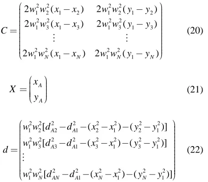
# # (20)

A A

x X

y ⎛ ⎞⎟ ⎜ ⎟

=_{⎜ ⎟⎜ ⎟}

⎜⎝ ⎠ (21)

2 2 2 2 2 2 2 2

1 2 2 1 2 1 2 1

2 2 2 2 2 2 2 2

1 3 3 1 3 1 3 1

2 2 2 2 2 2 2 2

1 1 1 1

[ ( ) ( )]

[ ( ) ( )]

[ ( ) ( )]

A A

A A

N AN A N N

w w d d x x y y

w w d d x x y y

d

w w d d x x y y

⎛ _{− − − − −} ⎞_⎟

⎜ _⎟

⎜ _⎟

⎜ ⎟

⎜ − − − − − ⎟

⎜ _⎟⎟

=⎜_{⎜ ⎟}

⎟

⎜ _⎟

⎜ ⎟

⎜ ⎟

⎜ _⎟⎟

⎜ − − − − −

⎝ ⎠

# (22)

If the number of the equations is larger than 2, x has no solution but approximation, so this problem is equivalent to solve normal equation:

,

T T

C CX=C b (23)

Then we can get:

1

( T ) T .

X= C C−C d (24)

Node A updates its position weight wAp by:

1

1 N

Ap i

i

w w

N =

=

∑

C. Localization From Only Two Neighbors

According to previous descriptions, a node requires at least three neighbors to locate by weight location estimation algorithm in the second phase. In other words, if it receives less than two neighbors, it can not locate its position. In order to solve this problem, we propose a method to obtain nodes' position if it only receives the signals of two neighbors.

Assume that node A has only two neighbors, node 1 and node 2, it may receive their position information

1 1

( ,x y), (x y₂, ₂). Using one ranging technology, the

distance dA1 and dA2 can be estimated by receiving

power strength.

Node A might also be located to another mirror position A' if d'A1 equals d'A2 . The geometric

relationship of these two possible position solutions A and A' is shown in Fig. 1.

According to the known information ( ,x y1 1), (x y2, 2),

1 A

d and d_A2, we can get two circle equations:

2 2 2

1 ( 1) ( 1)

A A A

d = x −x + y −y (26)

2 2 2

2 ( 2) ( 2)

A A A

d = x −x + y −y (27)

where (x_A,y_A) is the estimated node's position.

Subtracting equations (26) and (26), a straight line equation L can be obtained:

2 2 2 2 2 2

2 2 1 2 1 2

1 2 1 2

( ) ( )

( 2 2 ) ( 2 2 )

A A

A A

d d x x y y

x x x y y y

− − − − −

= − + + − + (28)

Based on equations (26), (27) and (28), the positions of node A or A' can be obtained.

After getting two possible positions, we still have to select the better one as estimation. The selection method is performed by the rule that finding the minimum distance between the estimated position and the initial position to be the better solution.

III. SIMULATION RESULTS

A. Simulation Setup

The well-known simulation tools ns-2 is used to validate the proposed scheme. We show some simulation results on different environments. In the initialization phase, only known nodes will broadcast packets to the network. This packet header contains whether the node is known node or not, known node's x and y coordinate and one-hop distance from known node computing. I

n the location estimation phase, all nodes (all unknown nodes and known nodes) flood packets to their neighbors, and this packet is called refine packet. Refine packet header also contains whether the node is known node or not, estimated or real x and y coordinate, and position

weight wp . Nodes also exchange information with

neighbors. After nodes receive packets from neighbors, they can use the ranging technology (e.g. RSSI) to estimate distances to their neighbors by measuring receiving power. The proposed algorithms ILA, LERA and ILA+LERA are compared with the node positioning algorithm (NPA) [9].

B. Performance Comparisons

In this scenario, we try to change connectivity which represents the average number of neighbors of nodes. Connectivity depends on the variance of the radio range, and we will observe the average position error and the number of nodes which can be located. The working area

in my simulation is 1000×1000m2. There are 100 nodes

in this working area with random placement.

0 10 20 30 40 50 60 70 80 90

5 10 15 20 25

Connectivity

Position error (R%)

NPA ILA LERA

Figure 2. Connectivity against position error.

0 20 40 60 80 100 120

5 10 15 20 25

Connectivity

Number of located nodes (%)

NPA ILA LERA

Figure 3. Connectivity against number of located nodes.

0 50 100 150 200 250

5 10 15 20 25

Connectivity

Position error (R%)

NPA with 5% known node ratio NPA with 10% known node ratio NPA with 20% known node ratio ILA+LERA with 5% known node ratio ILA+LERA with 10% known node ratio ILA+LERA with 20% known node ratio

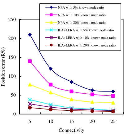
Figure 4. Connectivity against position error with different known node ratio.

that the proposed LERA algorithm outperforms than RPA and ILA. When connectivity is greater than 12, the position error decreases less than 50% radio range (R) for RPA. 50%R means half of the radio range. While for LERA, the position error is always less than 20% and it decreases fewer than 10%R with the connectivity increasing to 20. The position error of ILA is the worst in three algorithms.

Fig. 3 shows connectivity versus the number of located nodes. The same as Fig. 2, nodes with GPS ratio is 20%. When connectivity is only 5, the number of located nodes is greater than 70% whenever in the RPA, ILA or LERA. When connectivity is over 24, the number of located nodes is close to 100% in three algorithms. We can see the numbers of located nodes in the ILA and RPA are greater than that in LERA. This is because a node can not be refined in LERA when it has no at least two neighbors.

Then Fig. 4 shows connectivity versus the position error with different known node ratio for ILA+LERA and RPA. We can see when connectivity is only 5, the position error is greater than 200%R in 5% known node ratio and less than 100%R in 20% known node ratio for RPA. But when connectivity exceeds 24, the position

error decreases about 40%R with 20% known node ratio for RPA. While for the proposed ILA+LERA, we can observe the performance is obviously better than RPA. When connectivity is greater than 12, the position error decreases under 20%R whatever known node ratio is. And when connectivity exceeds 24, the position error is down to 5%R in 20% known node ratio. Fig. 4 obviously shows that our algorithm has better performance whatever connectivity is. The position error in the ILA+LERA is even decreases 10%R in 20% known node ratio. But when connectivity approaches 25, the position error converges to its lower bound, so the difference is not very apparent. The number of located nodes in proposed algorithm is greater than RPA algorithm, especially in lower connectivity.

In this scenario, we try to change the number of nodes, and observe the average position error and the number of nodes which can be located. The working area in our

simulation is 1000×1000m2. The radio range is 100m

and nodes are put in random placement.

Fig. 5 shows the number of nodes versus the position error for three algorithms with 20% known node ratio. When the number of nodes is 70, the position error of ILA approximates 100%R, while for ILA and LERA, the position errors are 72%R and 60% respectively. And the position error of LERA decreases down to half of ILA. If the number of nodes reaches 100, the position error of LERA is even less than 20%R, which is the lowest of three algorithms.

0 20 40 60 80 100 120 140 160 180

20 40 60 80 100

Number of nodes

Position error (R%)

NPA ILA LERA

Figure 5. Node number against position error.

0 20 40 60 80 100 120

20 40 60 80 100

Number of nodes

Number of located nodes (%)

NPA ILA LERA

Figure 6. Node number against number of located nodes.

0 20 40 60 80 100 120 140 160 180

20 40 60 80 100

Number of nodes

Po

sitio

n

erro

r (R%)

NPA with 5% known node ratio NPA with 10% known node ratio NPA with 20% known node ratio ILA+LERA with 5% known node ratio ILA+LERA with 10% known node ratio ILA+LERA with 20% known node ratio

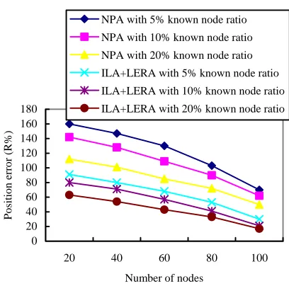
Figure 7. Node number against position error with different known node ratio.

0 50 100 150 200 250

20 40 60 80 100

Number of nodes

Network lifetime

NPA ILA+LERA

Figure 8. Network lifetime for different algorithms

LERA. And LERA outperforms than RPA. The reason is that the propose LERA can refine coordinate when a node has only two neighbors. And the weighted optimization scheme also improves the accuracy of location.

Then Fig. 7 shows the number of nodes versus the position error with different known node ratio for three algorithms. We can see when the number of nodes is very low, that the position error is over 110%R whatever known node ratio is for RPA. When the number of nodes is 40 with 20% known node ratio, the position error is about 100%R for RPA. And when the number of nodes is up to 100 in 20% known node ratio, the position error finally decreases approximately 50%R. For the proposed ILA+LERA, we discover the performance is obviously better than the RPA. When the number of nodes is greater than 40, the position error decreases down to 80%R whatever known node ratio is. When the number of nodes is up to 90, the position error is down to about 50% whatever known node ratio is. And when the number of nodes reaches 100 in 20% known node ratio, the position error excellently descends under 20%R.

Fig. 8 shows the results of network lifetime in different algorithms with different number of nodes. As shown in

Fig. 8, it is observed that the proposed ILA+LERA outperforms in terms of network lifetime irrespective of the number of nodes. For the algorithm NPA, the network lifetime greatly decreases to 58 when the number of nodes increases to 100. The reason is that the sensor nodes have to send more packets to exchange position information in NPA, thereby consuming more energy and the network lifetime decreases obviously when the number of layers increases. For the proposed ILA+LERA, the network lifetime decreases slightly when the number of nodes increasing. When the number of layers increases to 100, the network lifetime is 160 for ILA+LERA, which is about 3 times that of NPA. The results prove that the proposed positioning scheme can save node power and prolong network lifetime in positioning compared with NPA.

0 2000 4000 6000 8000 10000 12000 14000

5 10 20 30 40

Known node ratio (%) Total messages NPA

ILA+LERA

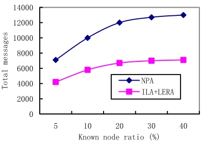
Figure 9. Total message exchanged for different algorithms.

ILA+LERA outperforms in terms of total message irrespective of the ratio of known nodes. For the algorithm NPA, the total message greatly increases to 13000 when the ratio of nodes increases to 40%. The reason is that the sensor nodes have to send more packets to exchange position information in NPA, thereby the total messages increases obviously when the ratio of known nodes increases to 40%. For the proposed ILA+LERA, the total messages increases slightly when the ratio of known nodes increasing. The reason is that the proposed scheme not only considers position information but also hop distance to known nodes, and it uses the weighted optimization method to decrease messages. When the ratio of known node increases to 40%, the total messages are 7100 for ILA+LERA, which is about half of NPA. The results prove that the proposed positioning scheme can select appropriate path and save power to prolong network lifetime in positioning compared with NPA.

IV. CONCLUSION AND FUTURE WORK

In this paper, an efficient intelligent position estimation method is proposed for distributed wireless sensor networks. The proposed scheme needs fewer known nodes without calculating relative positions. The proposed location algorithm includes two phases. The first phase adopts initialization location algorithm. Nodes with GPS broadcast their positions and one-hop distances, and then unknown nodes use information to calculate distances to nodes with GPS. Unknown nodes finally operates weighted estimation algorithm to calculate their initial positions. In the second phase, a weight optimized location algorithm is employed. Unknown nodes exchange information with their neighbors. According to neighbor is known node or not and unstable ranging measurement because of near or far, giving position weight and distance weight to represent their data accuracy. So they can operate modified weighted estimation algorithm to refine their positions repeatedly. Additionally, the proposed scheme also solves the location problem that a node only has two neighbors in the second phase. According to the simulation analyses, the proposed algorithm can decrease the average position

error down to 9%R and increase the average number of located nodes up to 78% when connectivity is greater than 12 in 20% known node ratio. On the side, when the number of nodes reaches 100 in 20% known node ratio, the average position error is under 20%R and the number of located nodes approximates 100%.

As a future research challenge, we envision that dynamic node positioning will be a promising direction for research.

ACKNOWLEDGMENT

This work is supported by Zhejiang natural science key foundation(Z1080232), national natural

science foundation of china(60873218), Education project of Zhejiang(20070597), and the foundation of science and technology department of Zhejiang province(2007C21009). . The authors are grateful for the anonymous reviewers who made constructive comments.

REFERENCES

[1] C.-Y. Chong, Srikanta P. Kumar, “Sensor Networks:

Evolution, Opportunities, and Challenges,” Proceedings of

the IEEE, vol. 91, no. 8, pp.1247-1256, 2003.

[2] A. Kemal, Y. Mohamed, Y. Waleed, “Positioning of base

stations in wireless sensor networks,” IEEE

Communications Magazine, v 45, n 4, pp. 96-102, 2007.

[3] J. Hightower and G. Borriello, “Location Systems for

Ubiquitous Computing,” Computer, vol. 34, no. 8, pp.

57-66, 2001.

[4] F. Reichenbach, D Timmermann, “Indoor Localization

with Low Complexity in Wireless Sensor Networks,” IEEE

Int. Conf Industrial Informatics, pp. 1018-1023, 2006.

[5] F. Yahya, “A new approximate positioning approach in

wireless sensor networks,” IEEE International Networking

and Communications Conference, pp. 138-143, 2008.

[6] K. Yu, M. Hedley, I. Sharp, “Node positioning in ad hoc

wireless sensor networks,” IEEE International Conference

on Industrial Informatics, pp. 641-646, 2006.

[7] N. Ha, K. Han, “Positioning method for outdoor systems in

wireless sensor networks,” Lecture Notes in Computer

Science, v4263, 2006, pp. 783-792.

[8] H.-C. Chu, R.-H Jan, “A GPS-less, outdoor,

self-positioning method for wireless sensor networks,” Ad Hoc

Networks, v 5, n 5, pp. 547-557, 2007.

[9] S. Susca, F. Bullo, S. Martinez, “Monitoring

environmental boundaries with a robotic sensor network,” IEEE Transactions on Control Systems Technology, v 16, n 2, pp. 288-296, 2008.

[10] C. D. Joseph, W. M. Michael, A. N. Mark, “A Theory for

Maximizing the Lifetime of Sensor Networks,” IEEE

Trans. on Commun., vol. 55, no. 2, pp. 323-232, 2007. [11] Mandala, Devendar Du, Xiaojiang; Dai, Fei; You, Chao,

“Load balance and energy efficient data gathering in

wireless sensor networks,” Wireless Communications and

Mobile Computing, v 8, n 5, pp. 645-659, 2008.

[12] S. Susca, F. Bullo, S. Martinez, “Monitoring environmental boundaries with a robotic sensor network,” IEEE Transactions on Control Systems Technology, vol. 16, no. 2, pp. 288-296, 2008.

in Sensor Networks,” 2005 IEEE/ACM International Conference on Distributed Computing in Sensor Systems (DCOSS ’05), June 2005, pp. 244-257.

[14] W.-C. Lee, Y. Xu, ‘Location-aware wireless sensor

networks,” IEEE International Conference on Mobile Data

Management, 2007, pp. 227-234.

[15] M. Zhang, C. C. Mun, A. L. Ananda, “Location-aided

topology discovery for wireless sensor networks,” IEEE

International Conference on Communications, 2008, pp. 2717-2722.

[16] S. Ray, W. Lai, I. C. Paschalidis, “Statistical location

detection with sensor networks,” IEEE Transactions on

Information Theory, v 52, n 6, pp. 2670-2683, 2006. [17] J. Arias, J. Lazaro, A. Zuloaga, et al. “GPS-less location

algorithm for wireless sensor networks,” Computer

Communications, v 30, n 14-15, pp. 2904-2916, 2007. [18] S.-M. Lee, H. Cha, Hojung; R. Ha, ‘Energy-aware location

error handling for object tracking applications in wireless

sensor networks,” Computer Communications, v 30, n 7,

pp. 1443-1450, 2007.

[19] S. Vural, E. Ekici, “Hop-distance based addressing and routing for dense sensor networks without location

information,” Ad Hoc Networks, v 5, n 4, pp. 486-503 2007.

[20] Q. Shi, S. Kyperountas, N. Correal, et al. “Performance analysis of relative location estimation for multihop

wireless sensor networks,” IEEE Journal on Selected

Areas in Communications, v 23, n 4, pp. 830-838, 2005.

[21] W.-W. Ji, Z. Liu, “Locating ineffective sensor nodes in

wireless sensor networks,” IET Communications, v 2, n 3,

pp. 432-439, 2008.

[22] Q. Fang, J. Gao, L. J. Guibas, “Locating and bypassing

holes in sensor networks,” Mobile Networks and

Applications, v 11, n 2, pp. 187-200, 2006.

[23] Fernand S. Cohen, D. C. Jaudelice; E. Taslidere, “Locating hot nodes and data routing for efficient decision fusion in

sensor networks,” Ad Hoc Networks, v 4, n 3, pp. 416-430,

2006.