University of Massachusetts Amherst University of Massachusetts Amherst
ScholarWorks@UMass Amherst
ScholarWorks@UMass Amherst
Doctoral Dissertations Dissertations and Theses
October 2019
Machine Learning Models for Efficient and Robust Natural
Machine Learning Models for Efficient and Robust Natural
Language Processing
Language Processing
Emma Strubell
Follow this and additional works at: https://scholarworks.umass.edu/dissertations_2
Part of the Artificial Intelligence and Robotics Commons
Recommended Citation Recommended Citation
Strubell, Emma, "Machine Learning Models for Efficient and Robust Natural Language Processing" (2019). Doctoral Dissertations. 1767.
https://scholarworks.umass.edu/dissertations_2/1767
This Open Access Dissertation is brought to you for free and open access by the Dissertations and Theses at ScholarWorks@UMass Amherst. It has been accepted for inclusion in Doctoral Dissertations by an authorized administrator of ScholarWorks@UMass Amherst. For more information, please contact
MACHINE LEARNING MODELS FOR EFFICIENT AND
ROBUST NATURAL LANGUAGE PROCESSING
A Dissertation Presented by
EMMA STRUBELL
Submitted to the Graduate School of the
University of Massachusetts Amherst in partial fulfillment of the requirements for the degree of
DOCTOR OF PHILOSOPHY September 2019
© Copyright by Emma Strubell 2019 All Rights Reserved
MACHINE LEARNING MODELS FOR EFFICIENT AND
ROBUST NATURAL LANGUAGE PROCESSING
A Dissertation Presented by
EMMA STRUBELL
Approved as to style and content by:
Andrew McCallum, Chair
Brendan O’Connor, Member
Mohit Iyyer, Member
Joe Pater, Member
Yoav Goldberg, Member
James Allan, Chair of the Faculty
ACKNOWLEDGEMENTS
I would not have been able to complete this dissertation without support from an enormous group of people, a subset of whom I will attempt to give credit here. I want to extend my deepest gratitude to my advisor Andrew McCallum for giving me a chance to try out this NLP thing, and for supporting me not only in my pursuits as a researcher, but also as an outdoorswoman. I am also very grateful to the rest of my thesis committee: Brendan O’Connor, Joe Pater, Mohit Iyyer, and Yoav Goldberg, for their thoughtful feedback on this work, that I wish I had solicited sooner! Much of this work was completed in collaboration with others, and I would particularly like to thank David Belanger, Luke Vilnis, Daniel Andor, David Weiss, Benjamin Roth and Thomas Kollar for helping me learn how to write a great paper and perform corre-spondingly careful and interesting research. I also want to thank Katherine Silverstein and Ananya Ganesh for their help not only as co-authors but also for enduring my mentorship as I hone those skills! Though we have not published papers together, I am also grateful for early pair-programming sessions with Jinho Choi and Alexandre Passos, where I learned how to engineer efficient NLP code. And although our work together is not included in this dissertation, I also want to thank Elsa Olivetti for being an awesome collaborator, and for showing me that you can be a super successful female scientist without sacrificing friendliness. I also want to extend my gratitude to mentors from my undergraduate career at UMaine who were indispensable for encouraging me to pursue a PhD, and helping me get into graduate school: David Hiebeler, Sudarshan Chawathe, Lawrence Latour and George Markowsky. Finally, I am extremely grateful for the boundless emotional and intellectual support from my best friends, Patrick Verga and Sara Merrick-Albano.
ABSTRACT
MACHINE LEARNING MODELS FOR EFFICIENT AND
ROBUST NATURAL LANGUAGE PROCESSING
SEPTEMBER 2019 EMMA STRUBELL B.S., UNIVERSITY OF MAINE
M.S., UNIVERSITY OF MASSACHUSETTS AMHERST Ph.D., UNIVERSITY OF MASSACHUSETTS AMHERST
Directed by: Professor Andrew McCallum
Natural language processing (NLP) has come of age. For example, semantic role labeling (SRL), which automatically annotates sentences with a labeled graph repre-sentingwho didwhat towhom, has in the past ten years seen nearly 40% reduction in error, bringing it to useful accuracy. As a result, a myriad of practitioners now want to deploy NLP systems on billions of documents across many domains. However, state-of-the-art NLP systems are typically not optimized for cross-domain robustness nor computational efficiency. In this dissertation I develop machine learning methods to facilitate fast and robust inference across many common NLP tasks.
First, I describe paired learning and inference algorithms for dynamic feature se-lection which accelerate inference in linear classifiers, the heart of the fastest NLP models, by 5–10 times. I then present iterated dilated convolutional neural networks
(ID-CNNs), a distinct combination of network structure, parameter sharing and train-ing procedures that increase inference speed by 14–20 times with accuracy matchtrain-ing bidirectional LSTMs, the most accurate models for NLP sequence labeling. Finally, I describe linguistically-informed self-attention (LISA), a neural network model that combines multi-head self-attention with multi-task learning to facilitate improved gen-eralization to new domains. We show that incorporating linguistic structure in this way leads to substantial improvements over the previous state-of-the-art (syntax-free) neural network models for SRL, especially when evaluating out-of-domain. I conclude with a brief discussion of potential future directions stemming from my thesis work.
TABLE OF CONTENTS
Page
ACKNOWLEDGEMENTS . . . .iv
ABSTRACT. . . v
LIST OF TABLES. . . .xi
LIST OF FIGURES. . . .xiii
CHAPTER INTRODUCTION. . . 1
1. BACKGROUND . . . 4
1.1 Machine learning models for sequence labeling in NLP . . . 4
1.1.1 Conditional probability models for sequence labeling . . . 4
1.1.2 Token representations and feature extraction . . . 5
1.1.2.1 Sparse, lexicalized feature functions . . . 6
1.1.2.2 Self-supervised pre-training and dense token embeddings . . . 8
1.1.2.3 Feed-forward and convolutional neural networks . . . 10
1.1.2.4 Recurrent neural networks . . . 12
1.1.2.5 Self-attention and Transformer networks . . . 14
1.2 Sequence labeling tasks in NLP . . . 16
1.2.1 Part-of-speech tagging . . . 16
1.2.2 Syntactic dependency parsing . . . 18
1.2.2.1 Graph-based dependency parsing . . . 19
1.2.2.2 Transition-based dependency parsing . . . 20
1.2.4 Semantic role labeling . . . 25
1.2.4.1 Predicate detection . . . 27
2. LEARNING DYNAMIC FEATURE SELECTION FOR FAST SEQUENTIAL PREDICTION . . . 29
2.1 Introduction . . . 29
2.2 Classification and Structured Prediction . . . 31
2.3 Linear models . . . 32
2.4 Method . . . 33
2.4.1 Definitions . . . 34
2.4.2 Inference . . . 34
2.4.3 Learning . . . 35
2.4.4 Learning the parameters . . . 36
2.4.5 Learning the template ordering . . . 37
2.4.5.1 Group Lasso and Group Orthogonal Matching Pursuit . . . 37
2.4.5.2 Sparse Regularized Group Orthogonal Matching Pursuit . . . 38
2.4.5.3 Wrapper Method . . . 39
2.5 Related Work . . . 40
2.6 Experimental Results . . . 42
2.6.1 Part-of-speech tagging . . . 42
2.6.1.1 Learning the template ordering . . . 45
2.6.2 Transition-based dependency parsing . . . 46
2.6.3 Named entity recognition . . . 48
2.6.4 Experiments: Learning Template Ordering . . . 48
3. FAST AND ACCURATE ENTITY RECOGNITION WITH ITERATED DILATED CONVOLUTIONS . . . 51
3.1 Introduction . . . 51
3.2 Background . . . 54
3.2.1 Conditional Probability Models for Tagging . . . 54
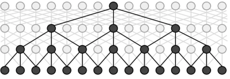
3.3 Dilated Convolutions . . . 55
3.4 Iterated Dilated CNNs . . . 57
3.4.1 Model Architecture . . . 57
3.4.2 Training . . . 58
3.5 Related work . . . 60
3.6 Experimental Results . . . 62
3.6.1 Data and Evaluation . . . 62
3.6.1.1 Optimization and data pre-processing . . . 63
3.6.1.2 Evaluation . . . 64
3.6.2 Baselines . . . 65
3.6.3 CoNLL-2003 English NER . . . 65
3.6.3.1 Sentence-level prediction . . . 65
3.6.3.2 Document-level prediction . . . 68
3.6.4 OntoNotes 5.0 English NER . . . 69
4. LINGUISTICALLY-INFORMED SELF-ATTENTION FOR SEMANTIC ROLE LABELING . . . 72
4.1 Introduction . . . 73
4.2 Model . . . 75
4.2.1 Self-attention token encoder . . . 77
4.2.2 Syntactically-informed self-attention . . . 78
4.2.3 Multi-task learning . . . 79
4.2.4 Predicting semantic roles . . . 80
4.2.5 Training . . . 81
4.3 Related work . . . 81
4.4 Experimental results . . . 83
4.4.1 Data and pre-processing details . . . 84
4.4.1.1 CoNLL-2012 . . . 85
4.4.1.2 CoNLL-2005 . . . 86
4.4.2 Optimization and hyperparameters . . . 86
4.4.3 Semantic role labeling . . . 87
4.4.4 Parsing, part-of-speech and predicate detection . . . 96
5. CONCLUSIONS AND FUTURE WORK . . . 101
5.1 Energy efficient NLP . . . 101
5.2 Optimization for extreme generalization . . . 104
5.3 Optimization and inference for multi-task learning . . . 106
5.4 Beyond English NLP . . . 107
5.5 Multi-task modeling for more robust document- and corpus-level reasoning . . . 108
LIST OF TABLES
Table Page
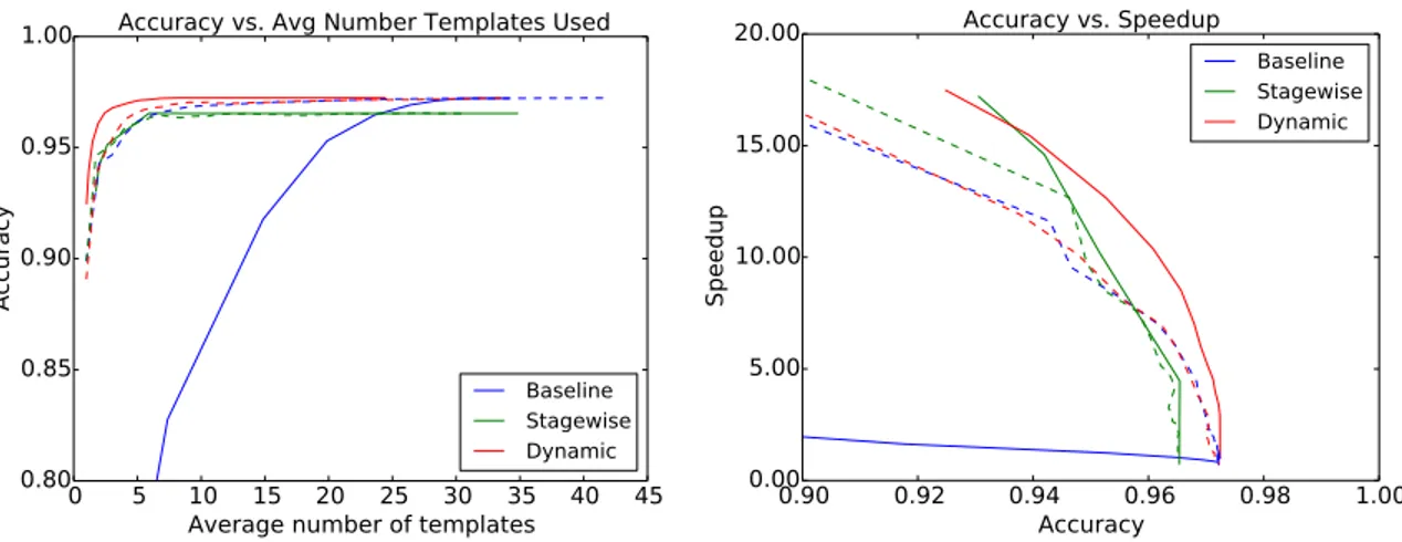
1.1 Statistics of NER datasets . . . 23 2.1 Comparison of our models using different marginsm, with speeds
measured relative to the baseline. We train a model as accurate as the baseline while tagging 3.4x tokens/sec, and in another model maintain >97% accuracy while tagging 5.2x, and >96%
accuracy with a speedup of 10.3x. . . 43 2.2 Comparison of our baseline and templated models using varying
marginsm and numbers of templates. . . 47 2.3 Comparison of our baseline and templated NER models using varying
marginm and number of templates. . . 48 2.4 Comparison of the wrapper method for learning template orderings
with group lasso and group orthogonal matching pursuit. Speeds are measured relative to the baseline, which is about 23,000
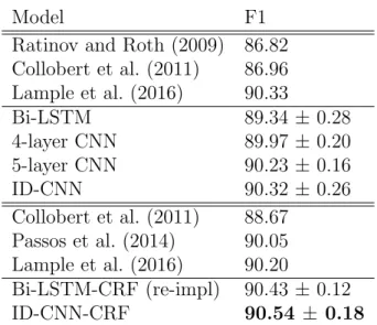
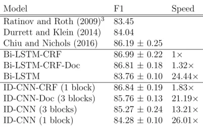
tokens/second on a 2.1GHz AMD Opteron machine. . . 49 3.1 F1 score of models observing sentence-level context. No models use
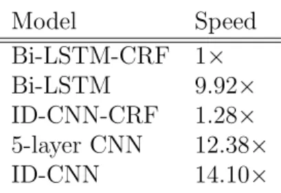
character embeddings or lexicons. Top models are greedy, bottom models use Viterbi inference . . . 66 3.2 Relative test-time speed of sentence models, using the fastest batch
size for each model.1 . . . 67
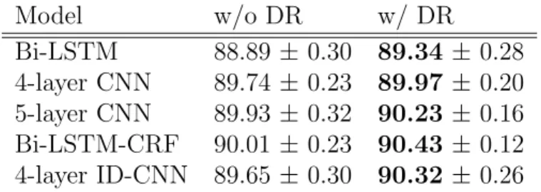
3.3 Comparison of models trained with and without expectation-linear
dropout regularization (DR). DR improves all models. . . 68 3.4 F1 score of models trained to predict document-at-a-time. Our
greedy ID-CNN model performs as well as the Bi-LSTM-CRF. . . 68 3.5 Comparing ID-CNNs with 1) back-propagating loss only from the
final layer (1-loss) and 2) untied parameters across blocks
3.6 Relative test-time speed of document models (fastest batch size for
each model). . . 69 3.7 F1 score of sentence and document models on OntoNotes. . . 70 4.1 Precision, recall and F1 on the CoNLL-2005 test sets. . . 87 4.2 Precision, recall and F1 on the CoNLL-2005 development set with
predicted and gold predicates. . . 88 4.3 Precision, recall and F1 on the CoNLL-2005 test set with gold
predicates. . . 89 4.4 Precision, recall and F1 on the CoNLL-2012 development and test
sets. Italics indicate a synthetic upper bound obtained by
providing a gold parse at test time. . . 90 4.5 F1 of GloVe models trained on only the news portion (nw) or all
domains, tested on all domains in the CoNLL-2012 development and test data. Italics indicate a synthetic upper bound obtained
by providing a gold parse at test time. . . 91 4.6 F1 of ELMo models trained on only the news portion (nw) or all
domains, tested on all domains in the CoNLL-2012 development and test data. Italics indicate a synthetic upper bound obtained
by providing a gold parse at test time. . . 92 4.7 Parsing (labeled and unlabeled attachment) and part-of-speech
accuracies attained by the models used in SRL experiments on
test datasets. . . 94 4.8 Predicate detection precision, recall and F1 on CoNLL-2005 and
CoNLL-2012 test sets. . . 96 4.9 Average SRL F1 on CoNLL-2005 and CoNLL-2012 for sentences
where LISA (L) and D&M (D) parses were correct (+) or
incorrect (–). . . 97 4.10 Comparison of development F1 scores with and without Viterbi
LIST OF FIGURES
Figure Page
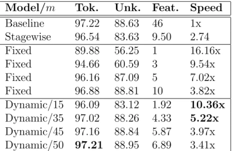
2.1 Left-hand plot depicts test accuracy as a function of the average number of templates used to predict. Right-hand plot shows speedup as a function of accuracy. Our model consistently achieves higher accuracy while using fewer templates resulting in
the best ratio of speed to accuracy. . . 44 2.2 Parsing speedup as a function of accuracy. Our model achieves the
highest accuracy while using the fewest feature templates. . . 47 3.1 A dilated CNN block with maximum dilation width 4 and filter width
3. Neurons contributing to a single highlighted neuron in the last
layer are also highlighted. . . 53 4.1 Word embeddings are input to J layers of multi-head self-attention.
In layerp one attention head is trained to attend to parse parents (Figure 4.2). Layer r is input for a joint predicate/POS classifier. Representations from layer r corresponding to predicted
predicates are passed to a bilinear operation scoring distinct predicate and role representations to produce per-token SRL
predictions with respect to each predicted predicate. . . 75 4.2 Syntactically-informed self-attention for the query word sloth.
Attention weights Aparse heavily weight the token’s syntactic
governor, saw, in a weighted average over the token values Vparse.
The other attention heads act as usual, and the attended representations from all heads are concatenated and projected through a feed-forward layer to produce the
syntactically-informed representation for sloth. . . 76 4.3 Bar chart depicting F1 scores on different CoNLL-2012 genres for a
model trained only on the newswire (nw) portion of the data,
with GloVe embeddings. . . 93 4.4 Bar chart depicting F1 scores on different CoNLL-2012 genres for a
4.5 F1 score as a function of sentence length. . . 98 4.6 CoNLL-2005 F1 score as a function of the distance of the predicate
from the argument span. . . 99 4.7 Performance of CoNLL-2005 models after performing corrections
from He et al. (2017). . . 100 4.8 Percent and count of split/merge corrections performed in Figure 4.7,
INTRODUCTION
Core natural language processing (NLP) tasks such as part-of-speech tagging, syn-tactic parsing and entity recognition have come of age thanks to advances in machine learning. For example, the task ofsemantic role labeling (annotatingwhodidwhat to
whom) has seen nearly 40% error reduction over the past decade. NLP has reached a level of maturity long-awaited by domain experts who wish to leverage natural language analysis to inform better decisions and effect social change. By deploying these systems at scale on billions of documents across many domains practitioners can consolidate raw text into structured, actionable data. These cornerstone NLP tasks are also crucial building blocks to higher-level natural language understanding (NLU) that our field has yet to accomplish, such as whole-document understanding and human-level dialog.
In order for NLP to effectively process raw text across many domains, we require models that are both robust to different styles of text and computationally efficient. The success described above has been achieved in those limited domains for which we have expensive annotated data; models that obtain state-of-the-art accuracy in these data-rich settings are typically neither trained nor evaluated for accuracy out-of-domain. Users also have practical concerns about model responsiveness, turnaround time in large-scale analysis, electricity costs, and consequently environmental conser-vation, but the highest accuracy systems also have high computational demand. As hardware advances, NLP researchers tend to increase model complexity in step.
The goal of my research is to facilitate large-scale, real-world natural language un-derstanding by developing machine learning algorithms for natural language
process-efficiency and robustness in NLP. To facilitate computational process-efficiency I describe new training and inference algorithms cognizant of strengths in the latest tensor process-ing hardware, and eliminate redundant computation through joint modelprocess-ing across many tasks. I also show that, with careful conditioning between tasks, modeling many tasks in a single model can improve robustness to new domains.
In Chapter 1 I provide an overview of the cornerstone NLP tasks typically mod-eled as sequence labeling, and the machine learning models for labeling text with those annotations that are the basis for my work. In Chapter 2 I present dynamic feature selection: paired learning and inference algorithms for significantly reducing computation in the linear classifiers at the heart of the fastest NLP models. This is accomplished by partitioning the features into a sequence of templates which are or-dered such that high confidence can often be reached using only a small fraction of all features. Parameter estimation is arranged to maximize accuracy and early confidence in this sequence. On typical benchmarking datasets for part-of-speech tagging, named entity recognition, and dependency parsing our technique preserves comparable ac-curacy to models using all features while reducing run-time by 5-10x. In Chapter 3 I describe Iterated Dilated Convolutional Neural Networks (ID-CNNs), a faster al-ternative to bidirectional LSTMs, the most accurate NLP sequence labeling models. In comparison to traditional CNNs, ID-CNNs have better capacity for large context and structured prediction. Unlike LSTMs whose sequential processing on sentences of length N requires O(N) time even in the face of GPU parallelism, ID-CNNs permit fixed-depth convolutions to run in parallel across entire documents. They embody a distinct combination of network structure, parameter sharing and training procedures that enable dramatic 14-20x test-time speedups while retaining accuracy compara-ble to the Bi-LSTM-CRF. Chapter 4 presents Linguistically-Informed Self-Attention (LISA), a neural network model that combines head self-attention with multi-task learning across dependency parsing, part-of-speech tagging, predicate detection
and SRL. Unlike previous models which require significant pre-processing to prepare syntactic features, LISA can incorporate syntax using merely raw tokens as input, encoding the sequence only once to simultaneously perform parsing, predicate detec-tion and role labeling for all predicates. Syntax is incorporated through the attendetec-tion mechanism, by training one of the attention heads to focus on syntactic parents for each token. We show that incorporating linguistic structure in this way leads to substantial improvements over the previous state-of-the-art (syntax-free) neural net-work models for SRL, especially when evaluating out-of-domain, where LISA obtains nearly 10% reduction in error while also providing speed advantages. In Chapter 5, I identify some limitations of my completed work, and describe a number of promising directions for future work inspired by the findings described herein.
CHAPTER 1
BACKGROUND
This thesis explores machine learning methods for the many different linguistic annotations that can be modeled as sequence labeling, assigning labels to the tokens in a sequence, where the sequence is typically a sentence or a document. Even more elaborate output structures such as entity spans and syntax trees can be extracted using sequence labeling techniques. In this chapter I first describe the basis for the sequence labeling machine learning models developed in this work (§1.1), and then I describe how these models are typically used to perform the five typical NLP pipeline tasks upon which I evaluate the models in this work: part-of-speech tagging, named entity recognition, syntactic dependency parsing, predicate detection and semantic role labeling (§1.2).
1.1
Machine learning models for sequence labeling in NLP
1.1.1 Conditional probability models for sequence labeling
Letx= [x1, . . . , xT] be our length-T sequence of input tokens andy= [y1, . . . , yT]
be per-token output tags. Let D be the domain size of each yi. We predict the most
likely y, given a conditional model P(y|x).
This work considers two factorizations of the conditional distribution. First, we have: P(y|x) = T Y t=1 P(yt|F(x)), (1.1)
where the tags are conditionally independent given some features for x. Given these features, O(D) prediction is simple and parallelizable across the length of the
se-quence. However, feature extraction may not necessarily be parallelizable. For exam-ple, RNN-based features require iterative passes along the length of x; see §1.1.2
We also consider a linear-chain CRF model that couples all of y together:
P(y|x) = 1 Zx T Y t=1 ψt(yt|F(x))ψp(yt, yt−1), (1.2)
where ψt is a local factor, ψp is a pairwise factor that scores consecutive tags, and
Zx is the partition function (Lafferty et al., 2001). Prediction in this model requires
global search using the O(D2T) Viterbi algorithm.
CRF prediction explicitly reasons about interactions among neighboring output tags, whereas prediction in the first model compiles this reasoning into the feature extraction step (Liang et al., 2008). The suitability of such compilation depends on the properties and quantity of the data. While CRF prediction requires non-trivial search in output space, it can guarantee that certain output constraints, such as for BIO tagging (Ramshaw and Marcus, 1999), will always be satisfied. It may also have better sample complexity, as it imposes more prior knowledge about the structure of the interactions among the tags (London et al., 2016). However, it has worse computational complexity than independent prediction.
1.1.2 Token representations and feature extraction
One of the most challenging aspects of machine learning is determining the best representation to use for the input. Typically raw inputs, such as an image or the words in a natural language sentence, are mapped to numeric representations suit-able as input to a machine learning model via a feature function, which we denote
F in Equations 3.1 and 3.2 above. The exact parameterization of F is the subject of extensive research in NLP, perhaps even more so than in other areas of machine learning research such as computer vision or speech processing. The inputs to
ma-inputs to the brain, whereas in NLP we take words as input, whose biological rep-resentations are far less understood (Embicka and Poeppel, 2015; Hubel and Wiesel, 1962; Kaas et al., 1999). As a result, while researchers in other areas can draw upon a great deal of knowledge from neuroscience and signal processing, in developing ar-tificial models for language understanding it is more challenging to take inspiration from what is known about biological systems. An additional challenge in NLP is the inherently discrete nature of text, compared to image and audio data where pro-cessing is inherently amenable to continuous representations. Since the most efficient optimization techniques operate in continuous space, in NLP we typically first map discrete representations of language (words and characters) to continuous represen-tations. Developing computationally efficient and robust parameterizations for F is the focus of much of this dissertation. In this section I describe many of the most typical parameterizations of F, upon which the work in this thesis builds. In the first subsection, I describe the sparse, lexicalized feature functions that drove the first wave of statistical models for NLP. The remaining sections explore more recent, highly data-driven approaches which use neural networks to build up rich features based on word similarity and context.
1.1.2.1 Sparse, lexicalized feature functions
The most straightforward representation for a token as input to a classifier is a one-hot vector indicating the word form for that token, typically normalized by e.g. removing casing, limiting to a fixed vocabulary, or more advanced morphological analysis. Indeed, in the first wave of statistical machine learning models for NLP, variants of this type of feature mapping, often referred to as lexicalized features, make up the vast majority of feature representations. Common lexicalized features include word form, affixes, capitalization patterns, discrete word cluster membership (Brown et al., 1992), and annotations from other models, such as part-of-speech tags
or word lemmas. These features are typically extracted not just for the current word, but also for adjacent words and combined to create n-gram features. Typical models for tagging and parsing consist of 50-100 of these different features mapping to hundreds of thousands to millions of binary features, resulting in a large, sparse binary representation for each token.
Once computed, these sparse feature representations are typically provided to a
linear model, the most basic classifier for sequence labeling. Given an input x∈ X, a set of labelsY, a feature map Φ(x, y), and a weight vectorw, a linear model predicts the highest-scoring label
y∗ = arg max
y∈Y
w·Φ(x, y). (1.3)
The parameter w is usually learned by minimizing a regularized (R) sum of loss functions (`) over the training examples indexed by i
w∗ = arg min w
X
i
`(xi, yi,w) +R(w).
Sparse lexicalized features are typically partitioned into a set offeature templates, so that the weights, feature function, and dot product factor as
w·Φ(x, y) = X
j
wj ·Φj(x, y) (1.4)
for some set of feature templates {Φj(x, y)}. A feature template corresponds to
a set of binary lexicalized features extracted by a single rule. For example, the feature template len3-suffix might correspond to all observed length-3 suffices in the training data for a given corpus. For a given token, a given feature template often maps to a one-hot vector (i.e. a given token has exactly one length-3 suffix),
in a lexicon). To avoid over-fitting, the range of templates like this is often limited such that only features observed more than some cutoff value (typically a single digit, depending on the size of the data) are considered.
1.1.2.2 Self-supervised pre-training and dense token embeddings
A recent and significant advance in NLP sequence labeling is self-supervised pre-training of dense vector token representations. Self-supervised refers to the practice of using token co-occurrences found in natural language text as a readily available training signal for learning token representations. This approach is based on the distributional hypothesis proposed by Harris (1951), which asserts that words with similar meaning are used in similar contexts. There are two main machine learning approaches to pre-training in this way: First, token representations may be context-independent, with a single representation learned for each item in the token vocabu-lary, shared across the entire corpus. When each token corresponds to a word these representations are known asword embeddings, a term and approach coined by Bengio et al. (2003), who used these representations as input to a neural network language model. Self-supervised pre-training of these word representations for downstream su-pervised tasks was proposed by Collobert et al. (2011) in their seminal multi-task neural network model for NLP sequence labeling. More recent popular examples of such pre-training of word representations include the word2vec context-bag-of-words (CBOW) and skip-gram with negative sampling (SGNS) training objectives (Mikolov et al., 2013), GloVe (Pennington et al., 2014), and structured word2vec (Ling et al., 2015a). The main differences between these techniques is whether token representa-tions are trained to be predictive of their context tokens (as in Mikolov et al. (2013)), or of co-occurrence counts (as in Pennington et al. (2014)), and whether the order-ing of context tokens is taken into account (Lorder-ing et al., 2015a). It has been shown that predict-based models (the SGNS objective in particular) is essentially
perform-ing implicit factorization of a word count co-occurrence matrix (Levy and Goldberg, 2014b). There have been many more specialized variants of embeddings trained for better performance on specific tasks, such as word representations that take into ac-count syntactic (Levy and Goldberg, 2014a) or semantic (Rothe and Sch¨utze, 2015) information.
More recently, advances in hardware and methodology have enabled improved pre-training ofcontext-dependent token representations, where a given token embed-ding is a function of its exact context in a sentence or document. These models are typically trained using a language-modeling objective similar to previous approaches, except that token representations are not shared across each instance in the corpus, but instead vary depending on the specific sentence or document containing a to-ken. These models typically employ multiple neural network layers to build a token representation that effectively incorporates multiple aspects of its context, and the representations at each layer for a given token can be combined in different ways, often via task-dependent parameters that are fine-tuned in a secondary training step. The first of these models to achieve great success by demonstrating large accuracy gains across many NLP sequence labeling tasks is the ELMo model (Peters et al., 2018), which consists of multiple LSTM neural network layers (§1.1.2.4), where the first layer builds token representations from character embeddings. Subsequent mod-els include BERT (Devlin et al., 2019), which uses the Transformer neural network architecture (§1.1.2.5) and a different language modeling training objective, GPT and GPT-2 (Radford et al., 2019), which are also Transformer-based with different train-ing. In contrast with the word embedding models described in the previous section and the ELMo model which uses character embeddings, BERT and other models use
wordpiece embeddings (Schuster and Nakajima, 2012; Wu et al., 2016), which find a middle ground between word and character embeddings, which compared to word embeddings have been found to improve generalization (by removing out-of-domain
words and capturing morphology), require a reduced memory footprint, but require increased computation to obtain word embeddings and consequently result in slower inference. A fixed vocabulary of wordpieces are obtained by computing the most common word subsequences in a training corpus, such that the fixed set of word-pieces can be combined to form any word, but the number of wordword-pieces required to create a word on average is minimized. While this work does contain experiments incorporating ELMo embeddings and therefore character embeddings, since the focus of this work is the morphologically-poor English language all other experiments in this document use pre-trained word embeddings.
1.1.2.3 Feed-forward and convolutional neural networks
The most straightforward neural network extension of the basic linear models described in§1.1.2.1 is thefeed-forward neural network. Feed-forward networks simply add additional layers of processing to the input before classification via multiple linear transformations, each followed by anonlinearity,1 a non-linear function applied
output. For example, a two-layer feed-forward network applied to an input xt with
transformations Wc(1) and Wc(2) and nonlinearity function σ producing the output
representation ct:
ct=σ(Wc(2)σ(W
(1)
c xt)), (1.5)
Common nonlinearities include tanh, sigmoid, and the rectified linear (ReLU) func-tions. The linear transformations Wc may increase the dimensionality of the input,
or decrease it. Typically the dimension of these transformations is treated as a model hyperparameter.
1Without the nonlinearity, multiple applications of linear layers are functionally equivalent to a single linear layer.
Convolutional neural networks (CNNs) in NLP are a straightforward extension of feed-forward networks which simply apply the linear transformation to a window of adjacent tokens, rather than a single token on the input. In NLP convolutions are typically one-dimensional, applied to a sequence of vectors representing tokens rather than to a two-dimensional grid of vectors representing e.g. pixels. In this setting, a convolutional neural network layer is equivalent to applying a linear transformation to a sliding window of width r tokens on either side of each token in the sequence. Here, and throughout the chapter, we do not explicitly write the bias terms in linear transformations. The sliding-window representation ct for each token xt is:
ct=Wc[xt−r;. . .;xt−1;xt;xt+1;. . .;xt+r] (1.6)
where [·;·] denotes vector concatenation. Often, multiple convolutional layers are stacked, with the output representation from one layer being provided as input to the next layer, in order to build up richer representations incorporating information from a wider context. As with feed-forward networks, a nonlinearity must be applied after each convolutional layer. In a stacked CNN, the effective size of the context observed by a token at layerk with input radiusr is given by 2kr+ 1, i.e. the width grows by 2r at each layer.
In NLP CNNs are most commonly applied to (1) character-level modeling (com-posing characters into token representations to capture morphological information and allow for classification of unseen words) and (2) sentence-level classification, rather than token-level classification. This is because, like linear and feed-forward models, even when stacked as described above they are limited to a fixed-width window of con-text. In the next sections I will describe neural network models that can incorporate context from an entire sequence into the representation for each token. These models are typically less computationally efficient than linear, feed-forward and convolutional
1.1.2.4 Recurrent neural networks
Recurrent neural networks incorporate context from the entire sequence by pro-cessing tokens incrementally in order, maintaining a state vector htthat incorporates
information at each timestep of the input:
ht=RN N(xt, ht−1) =Wh[xt;ht−1] (1.7)
where [·;·] denotes again vector concatenation. For sequence labeling, it has been shown that incorporating both right- and left-context in a bidirectional model is beneficial (Schuster and Paliwal, 1997). Bidirectional models combine RNNs in the forward and backward direction by concatenating their hidden representations at each timestep: ht= [ ←−−− RN N(xt, ←− ht+1); −−−→ RN N(xt, − → ht−1)] (1.8)
In practice, higher accuracy for challenging tasks can be obtained by stacking multiple RNNs, where subsequent RNNs take as input at each timestep the hidden states from the previous RNN, rather than the raw input representations xt.
Vanilla RNNs, that is RNNs that use just a single linear transformation to inte-grate information from the current timestep with the hidden state, have been repeat-edly shown to effectively model time-dependent data, such as natural language text. However, as the sequence length increases, long term dependencies can be lost due to the vanishing gradient problem (Hochreiter, 1998). The Long Short Term Mem-ory (LSTM) variant of RNNs was designed to overcome this shortcoming (Hochreiter and Schmidhuber, 1997). The LSTM incorporates three additional matrices inside the recurrence which act as a gating mechanism, selectively allowing information flow from previous timesteps as a function of the current timestep. The gates ft, it and
ot are defined as functions of the input xt and previous hidden representationht−1 as
follows:
ft=σg(Wfxt+Ufht−1+bf) (1.9)
it=σg(Wixt+Uiht−1+bi) (1.10)
ot=σg(Woxt+Uoht−1+bo) (1.11)
matrices W and U and bias vectors b are all model parameters learned through supervised training. σg denotes the sigmoid activation function, which normalizes
the outputs to have values in [0,1]. These representations are combined to produce the hidden representation ht as follows:
ct =ft◦ct−1+it◦σc(Wcxt+Ucht−1+bc) (1.12)
ht =ot◦σh(ct) (1.13)
where ◦ denotes element-wise vector multiplication. Activations σc and σh use the
tanh function to normalize outputs into the range [−1,1]. The LSTM out-performs out-perform the vanilla RNN as a token encoder for various NLP tasks, and as a result has become the de facto token encoder in NLP.
There exist many other variants of recurrent neural network architectures with varying internal structure for combining context state and input such as GRUs (Cho et al., 2014), Skip RNNs (Campos et al., 2018), highway LSTMs (Zhang et al., 2015b) or stacked LSTMs with different patterns of connectivity (Zhou and Xu, 2015a). The work in this document implements only the most common LSTM architecture, so the reader is referred to the original works for detailed discussion of these alternatives.
1.1.2.5 Self-attention and Transformer networks
Self-attention is a new alternative to recurrent architectures for incorporating in-formation from the entire sequence into each token representation. Unlike recurrent networks, self-attention can process all tokens in a sequence at once in parallel, and are thus very efficient on modern tensor processing hardware such as GPUs and TPUs. This contextual information is incorporated through a neural attention mechanism, essentially a context-dependent weighted average, where the term self-attention sim-ply indicates that the weighted average for a given token is over the same sentence as the token is located. In this work, experiments focus on the Transformer instanti-ation of self-attention (Vaswani et al., 2017). Rather than incrementally building up context from each token in order, the Transformer model uses stacked layers each con-sisting of multiple self-attention functions to build up rich representations of tokens in context.
More specifically, the Transformer model works as follows. Input token represen-tations xt are each projected to a representation that is the same size as the output
of the self-attention layers. Importantly, a positional encoding vector computed as a deterministic sinusoidal function oftis added to the input, since the self-attention has no innate notion of token position. Alternatively, position embeddings can be used to supply this information to the model, with the downside that position embeddings are limited to a maximum distance determined at train time.
This token representation is provided as input to a series of J residual multi-head self-attention layers with feed-forward connections. Denoting the jth self-attention layer asT(j)(·), the output of that layerst(j), andLN(·) layer normalization (Ba et al., 2016), the following recurrence applied to initial inputc(tp):
gives final token representations s(tj). Each T(j)(·) consists of: (a) multi-head self-attention and (b) a feed-forward projection.
The multi-head self attention consists of H attention heads, each of which learns a distinct attention function to attend to all of the tokens in the sequence. This self-attention is performed for each token for each head, and the results of theH self-attentions are concatenated to form the final self-attended representation for each token.
Specifically, consider the matrix S(j−1) of T token representations at layer j − 1. For each attention head h, we project this matrix into distinct key, value and query representations Kh(j), Vh(j) and Qh(j) of dimensions T ×dk, T ×dq, and T ×dv,
respectively. We can then multiplyQ(hj)byKh(j)to obtain aT×T matrix of attention weights A(hj) between each pair of tokens in the sentence. Following Vaswani et al. (2017) we perform scaled dot-product attention: We scale the weights by the inverse square root of their embedding dimension and normalize with the softmax function to produce a distinct distribution for each token over all the tokens in the sentence:
A(hj)= softmax(d−k0.5Q(hj)Kh(j)T) (1.15)
These attention weights are then multiplied by Vh(j) for each token to obtain the self-attended token representationsMh(j):
Mh(j) =Ah(j)Vh(j) (1.16)
Row t of Mh(j), the self-attended representation for token t at layer j, is thus the weighted sum with respect to t (with weights given by A(hj)) over the token represen-tations in Vh(j).
repre-each followed by leaky ReLU activations (Maas et al., 2013). We add the output of the feed-forward to the initial representation and apply layer normalization to give the final output of self-attention layer j, as in Eqn. 1.14.
1.2
Sequence labeling tasks in NLP
The previous section described many of the most common machine learning ap-proaches to sequence labeling in NLP. In this section, I give an overview of many of the most common token-level sequence labeling tasks in NLP: part-of-speech tagging, named entity recognition, syntactic dependency parsing, semantic role labeling and predicate detection. These are all the tasks upon which the models described in this work are evaluated. Although this is far from an exhaustive list of all the annotations studied in NLP and desired by practitioners, these make up a representative suite of the most common tasks included in a typical NLP pipeline alongside (typically deterministic) tokenization and sentence segmentation. The majority of other de-sired token annotations can be obtained using similar techniques, simply applied to different label sets.
1.2.1 Part-of-speech tagging
Part-of-speech tagging is the task of annotating tokens with their part-of-speech tags, such as noun, verb, adjective, et cetera. There exist distinct sets of tags for many different languages, as well as a set of universal part-of-speech tags which can be used for multilingual modeling (Petrov et al., 2012). Since this work is focused on English NLP, we focus experiments on the annotations in the Wall Street Journal portion of the Penn TreeBank corpus (Marcus et al., 1993b), a collection of 2,499 news articles (about 1 million tokens) from the 1989 Wall Street Journal newspaper annotated with Treebank II style syntax trees (Bies et al., 1995).
This corpus defines 49 part-of-speech tags for English, differentiating between verb tenses, singular and plural nouns, and some types of punctuation.2 The dataset is
divided into 24 sections. In the typical evaluation setup for part-of-speech tagging, sections 0–18 are used for training, sections 19–21 for development, and sections 22–24 as test data. Each token is annotated with exactly one part-of-speech tag, and models are typically evaluated in terms of per-token and sometimes per-sentence accuracy. Modern models typically achieve accuracy between 97–98%, approximately the limit of human annotators for this task (Manning, 2011). Automatic part-of-speech annotations can be obtained as part of syntactic constituency parsing, or labels can be assigned to tokens by simple multi-class classification for each token, which is the approach we take in this work. Typically part-of-speech tagging is the first step after tokenization and sentence segmentation in an English NLP pipeline.
The earliest machine learning models for part-of-speech tagging which can ob-tain accuracy close to today’s state-of-the-art are generative hidden Markov models (HMMs) (Charniak et al., 1993; Church, 1989). More recently part-of-speech tagging models have trended towards discriminative logisic regression (log-linear) models, also known as maximum entropy or MaxEnt models (Ratnaparkhi, 1996; Toutanova et al., 2003). These are still among the most common part-of-speech tagging models found in off-the-shelf NLP tools. More recently, feed-forward (Collobert et al., 2011) and recurrent neural networks have been shown to obtain state-of-the-art performance for part-of-speech tagging (Ling et al., 2015b), though for English the accuracy obtained by these more complex models over simpler linear models is often negligible.
2See the annotation guidelines for more details: https://catalog.ldc.upenn.edu/docs/
1.2.2 Syntactic dependency parsing
The next step in typical NLP pipelines following part-of-speech tagging is syntactic parsing, which induces a tree structure over the tokens indicating syntactic relations in the sentence. In this work we focus on syntactic dependency parsing, where this tree is made up of edges assigned between tokens in the sentence; no additional (internal) nodes e.g. representing phrases are added to the representation. Each token is assigned one parent, which is another token in the sentence, and one token is designated as the root of the sentence, which is to assigned itself as a parent, or a dummy “root” token. Dependency parsing has been increasingly adopted over constituency parsing due to its more favorable run-time efficiency — For a sentence of lengthN tokens, expectedO(N) parsing time for greedy, transition-based projective parsing and O(N2) for non-projective parsing (Nivre, 2003, 2009), versus O(N3) for
CKY — and simply implemented models, though information is lost when converting from constituency to more simple dependency parse structure. Currently, the most accurate machine learning model for dependency parsing is a constituency parser whose outputs are converted to dependency trees post-hoc (Dyer et al., 2016).
The benchmark dataset for English syntactic parsing is also the Wall Street Jour-nal portion of the Penn TreeBank (see §1.2.1). For dependency parsing the con-stituency trees are converted to dependencies with a deterministic set of head rules, which can be used to identify the head of a phrase, and an associated mapping to labels on the induced dependency edges. The sets of head rules most commonly used in NLP are the Collins or Yamada and Matsumoto head rules (Collins, 1999; Yamada and Matsumoto, 2003), and the head rules for the Stanford Dependencies framework (de Marneffe and Manning, 2008). Currently, Stanford Dependencies v3.3 is the de-pendency framework of choice for syntactic parsing. The split of the Penn TreeBank used for dependency parsing differs from that used for part-of-speech tagging: sec-tions 2–21 are used for training, section 23 is used for evaluation, and secsec-tions 22 and,
more recently in response to highly data driven models, 24 are used for development (Weiss et al., 2015). A model for dependency parsing may or may not include labels on the edges, though recently it is typical for dependency models to perform labeled parsing. Dependency parsing is typically evaluated using labeled attachment score (LAS), unlabeled attachment score (UAS), and sometimes label score (LS). Each of these are measures of per-token accuracy. Labeled attachment score counts a token as correct only if its head and label are assigned correctly. Unlabeled attachment score considers only whether a token’s head was assigned correctly, and label score consid-ers only whether the label on the edge is correct. In English, punctuation tokens3 are
typically excluded from evaluation due to inconsistencies in the Penn TreeBank data on where punctuation tokens should attach.
There are two main algorithms for obtaining dependency parses of sentences:
graph-based dependency parsing and transition-based dependency parsing. We de-scribe these two techniques below. Both are used in different models dede-scribed in this work.
1.2.2.1 Graph-based dependency parsing
Graph-based approaches to dependency parsing directly predict edges between tokens in the syntactic dependency tree. The most common approach to graph-based dependency parsing with neural networks is thefirst-order edge-factored model, which produces representations for the potential edge between each pair of tokens in the sentence, then uses those representations to predict exactly one edge going into each token (i.e., each token has exactly one head). Higher-order models have been shown to increase graph-based parsing accuracy over these simpler models (Bohnet, 2010; Carreras, 2007; Koo and Collins, 2010), but since the rise of neural network models it
is yet to be shown that explicitly modeling higher-order dependency graph structure improves accuracy in relatively data-rich settings such as English news text.
Since greedy one-best prediction does not guarantee that the predictions form a well-structured tree4, typically a post-processing step is performed to induce a tree
from the model predictions, such as computing the maximum spanning tree given edge scores output by the model (McDonald et al., 2005). Alternatively, the model can be trained with a structured objective that produces a tree during inference, such as the matrix-tree or Chu-Liu-Edmonds algorithm (Koo et al., 2007) which runs in O(T2) time for a length T sentence. These approaches produce non-projective
dependency trees, or trees that may have necessarily crossing dependencies when drawn on a plane. For highly projective languages such as English or Chinese, it may be desirable to constrain the inference algorithm to predict only projective trees; adding such a structural inductive bias can be particularly helpful in low-data settings. Eisner (1996) proposed dynamic programming algorithms which guarantee projective outputs, at the cost of slower O(T3) runtime efficiency.
1.2.2.2 Transition-based dependency parsing
As opposed to graph-based parsing where dependencies are predicted directly that form a tree, transition-based parsers instead predict a series of transitions, or shift-reduce operations, which incrementally build up a tree by adding edges between tokens and pushing and popping from a stack. This type of parsing is also known as shift-reduce or incremental parsing. Some of the first neural network-based dependency parsers were transition-based parsers (Andor et al., 2016; Chen and Manning, 2014; Weiss et al., 2015), which used feed-forward networks. More recently, these transition-based approaches, which run very fast on CPU hardware, have been eschewed in favor of more accurate graph-based neural network approaches (Clark et al., 2018; Dozat
and Manning, 2017; Kiperwasser and Goldberg, 2016), which can be performed more efficiently on GPU hardware.
More specifically, transition-based parsing algorithms typically use a stack and a buffer of tokens, combined with a specific set of transitions. The buffer is initialized to contain the tokens in the sentence, and the stack is initialized to be empty. At a given step during prediction, given (features of) the state of the stack and the buffer, a model predicts the next transition, which is performed, and this is repeated until the stack and buffer are empty. For a given transition system, the gold-standard series of transitions can be deterministically generated from the gold-standard parse tree.
Different transition systems are used for projective and non-projective parsing. The most basic transition system for projective parsing is called the arc-standard
transition system (Nivre, 2003). This system defines three transitions: left-arcl,
right-arclandshift. shiftpushes the first token on the buffer to the stack.
left-arcl adds a dependency arc (with label l) from the token at the top of the buffer to
the top of the stack, and pops the stack. right-arcl adds a labeled dependency arc
from the token at the top of the stack to that at the top of the buffer, pops the stack, and replaces the top of the buffer with the token that was at the top of the stack.
Another popular transition system for projective parsing is the arc-eager transi-tion system, which is designed to produce more plausible incremental (partial) trees by adding both left and right edges as soon as the head and dependent tokens are avail-able, as opposed to in the arc-standard system, where either left- or right-dependents (typically right) are not attached to heads until each token has found all of its de-pendents (Nivre, 2004). In other words, the arc-standard system performs purely bottom-up parsing, while the arc-eager system combines bottom-up and top-down parsing. The arc-eager transition system adds a reduce transition, which simply pops the stack, and uses a modified right-arc transition, which makes the top of
the stack the head of the token at the top of the buffer, then pushes the token at the top of the buffer to the stack.
This description focuses on projective transition systems since the focus of this work is English, in which the vast majority of sentences are projective.5 There also
exist a number of transition systems for producing non-projective parses, most notably Nivre’s list-based (Nivre, 2008), and swap-based approaches (Nivre, 2009).
1.2.3 Named entity recognition
Named entity recognition is the task of identifying typed spans of tokens corre-sponding to named entities, such as Washington and United States of America. The two most commonly used benchmark datasets for English named entity recognition are the CoNLL 2003 shared task (Sang and Meulder, 2003) and the CoNLL 2012 (Pradhan et al., 2012) subset6 of the OntoNotes corpus v5.0 (Hovy et al., 2006;
Prad-han et al., 2006). Entities in the CoNLL 2003 corpus are labeled with one of four types: per, org, loc or misc, with a fairly even distribution over the four entity types. OntoNotes contains a larger and more diverse set of 19 different entity types, adding: ordinal, product, norp, work of art, language, money, percent, car-dinal, gpe, time, date, facility, law, event and quantity. The OntoNotes corpus also covers a wider range of text genres, including telephone conversations, web text, broadcast news and translated documents, whereas the CoNLL-2003 text covers only newswire. The sizes of the two corpora in terms of documents, sentences, tokens and entities are given in Table 1.1.
Named entity recognition is often modeled similarly to part-of-speech tagging, where each token is assigned a label, with non-entity tokens receiving the O label.
5Chen and Manning (2014) report that 99.9% of syntax trees converted to Stanford dependencies in the Penn TreeBank training data are projective.
6The CoNLL 2012 split includes pivot text, which is typically excluded from the data for training and evaluating named entity recognition models.
Dataset Train Dev Test CoNLL-2003 Tokens 204,567 51,578 46,666 Sentences 14,041 3,250 3,453 Documents 945 215 230 Entities 23,499 5,942 5,648 OntoNotes 5.0 Tokens 1,088,503 147,724 152,728 Sentences 59,924 8,528 8,262 Documents 2,483 319 322 Entities 81,828 11,066 11,257 Table 1.1: Statistics of NER datasets
Typically a boundary encoding is used to assist in classification, i.e. the label of the first token in an entity span is pre-pended withB-and remaining labels in that span pre-pended with I; this is known as BIO or IOB encoding (Ramshaw and Marcus, 1999). Ratinov and Roth (2009) report that, for non-structured models, a slightly more elaborate BILOU (also known as IOBES) encoding, which additionally distin-guishes between the final token (L) in a span, and single-token spans (U) out-performs the more basic BIO encoding scheme.
Named entity recognition is typically evaluated using F1 score, which is the har-monic mean of precision and recall. Precision measures, of the spans that were pre-dicted, how many were correct, and is calculated as the number of true positives divided by the total number of predicted spans. Recall measures how many of the correct spans were predicted, and is computed as the number of true positives di-vided by the total number of spans in the gold standard data. Precision and recall are computed at the segment level, rather than at the token level, so all the tokens in a span need to be identified correctly in order for that span to be considered correct (a true positive).
LSTMs (Hochreiter and Schmidhuber, 1997) were used for NER as early as the CoNLL shared task in 2003 (Hammerton, 2003), but due to lack of hardware, like many other neural network approaches at the time the model was out-performed
by approaches using graphical models with lexicalized features based on word type, affixes and capitalization, and generous use of lexicons (Luo et al., 2015; McCallum and Li, 2003; Passos et al., 2014). (Durrett and Klein, 2014) leverages the parallel co-reference annotation available in the OntoNotes corpus to predict named entities jointly with entity linking and co-reference.
More recently, a wide variety of neural network architectures for NER have been proposed. Collobert et al. (2011) employ a one-layer CNN with pre-trained word embeddings, capitalization and lexicon features, and CRF-based prediction. Huang et al. (2015) achieved state-of-the-art accuracy on part-of-speech, chunking and NER using a Bi-LSTM-CRF. Lample et al. (2016) proposed two models which incorporated Bi-LSTM-composed character embeddings alongside words: a Bi-LSTM-CRF, and a greedy stack LSTM which uses a simple shift-reduce grammar to compose words into labeled entities. Their Bi-LSTM-CRF obtained the state-of-the-art on four languages without word shape or lexicon features. Ma and Hovy (2016) use CNNs rather than LSTMs to compose characters in a Bi-LSTM-CRF, achieving state-of-the-art per-formance on part-of-speech tagging and CoNLL NER without lexicons. Chiu and Nichols (2016) evaluate a similar network but propose a novel method for encod-ing lexicon matches, presentencod-ing results on CoNLL and OntoNotes NER. Yang et al. (2016) use GRU-CRFs with GRU-composed character embeddings of words to train a single network on many tasks and languages.
There have been some approaches showing that incorporating document-level con-text can help named entity recognition. Ratinov and Roth (2009) incorporate doc-ument context in their greedy model by adding features based on tagged entities within a large, fixed window of tokens. Bunescu and Mooney (2004) pose an undi-rected graphical model over all entities in a document, Sutton and McCallum (2004) employ a skip-chain CRF to model factors between entities while supporting efficient
inference, and Finkel et al. (2005) enforce non-local constraints during inference in a CRF.
1.2.4 Semantic role labeling
Semantic role labeling (SRL) is often described as identifying who did what to
whom. More precisely, given the (most often verbal) predicates in a sentence, semantic role labeling is the task of, for each predicate, identifying the typed spans of text corresponding to the arguments participating in that predicate’s semantic frame.
The CoNLL-2005 shared task (Carreras and M`arquez, 2005) spearheaded machine learning approaches to SRL by providing a version of the Wall Street Journal portion of the Penn TreeBank corpus annotated with predicate-argument structure in the style of PropBank (Palmer et al., 2005). PropBank labels arguments with six predicate-specific labelsarg0–arg5, known ascore arguments as well as 18 types of modifiers, e.g. argm-mnr,argm-neg. More details can be found in the PropBank annotation guidelines (Bonial et al., 2010). This dataset is one of the main benchmark datasets for SRL, alongside the CoNLL 2009 shared task data (Hajiˇc et al., 2009), which also uses PropBank predicate-argument structure, but annotates only the syntactic heads of phrases, rather than entire spans of text, and the CoNLL 2012 shared task, which includes the annotations from CoNLL 2005 but adds a number of documents from different domains in the OntoNotes corpus, such as broadcast news, telephone conversations and discussion forums.
Since far more annotations are available using PropBank frames, the majority of NLP research has focused on that formalism. Other popular and practical formalisms include VerbNet (Kipper-Schuler, 2005), which annotates arguments with descriptive labels that are shared across all predicates, such astheme,agentandinstrument. FrameNet (Baker et al., 1998) similarly annotates arguments with labels that are shared across predicates, but FrameNet labels are far more fine-grained than VerbNet
(e.g. mover, vehicle), making it challenging to train a machine learning model for tagging. All of these frameworks extend the verb classes defined by Levin (1993).
There are two main approaches to semantic role labeling: Most recent models identify argument spans for a predicate using token-level tagging with BIO-encoded labels, similar to named entity recognition (He et al., 2017; Marcheggiani et al., 2017; Tan et al., 2018; Zhou and Xu, 2015b). Tags can be predicted independently, or more often decoding can be performed using the Viterbi algorithm. Rather than tagging tokens, another approach is to perform span-level tagging, by considering all possible spans within a sentence up to a maximum length, building feature representations for each span, then assigning labels directly to spans (He et al., 2018; Ouchi et al., 2018). In both cases, SRL is typically evaluated using span-level F1, like named entity recognition.
In NLP pipelines, SRL typically comes after syntactic parsing, following biologically-inspired intuitions that syntactic processing occurs before semantics. Early machine learning approaches to SRL (Johansson and Nugues, 2008; Pradhan et al., 2005; Sur-deanu et al., 2007; Toutanova et al., 2008) focused on developing rich sets of linguistic features as input to a linear model, often combined with complex constrained infer-ence e.g. with an ILP (Punyakanok et al., 2008). T¨ackstr¨om et al. (2015) showed that constraints could be enforced more efficiently using a clever dynamic program for exact inference. While most of these techniques require a predicted parse as input, Sutton and McCallum (2005) modeled syntactic parsing and SRL jointly, and Lewis et al. (2015) jointly modeled SRL and CCG parsing.
Collobert et al. (2011) were among the first to use a neural network model for SRL, a CNN over word embeddings combined with globally-normalized inference. However, their model failed to out-perform non-neural models, both with and without multi-task learning with other NLP tagging multi-tasks. FitzGerald et al. (2015) successfully
employed neural networks by embedding lexicalized features and providing them as factors in the model of T¨ackstr¨om et al. (2015).
Recently there has been a move away from SRL models which explicitly incor-porate syntactic knowledge through features and structured inference. Zhou and Xu (2015b), Marcheggiani et al. (2017) and He et al. (2017) all use variants of deep LSTMs with constrained decoding, while Tan et al. (2018) apply self-attention to obtain state-of-the-art SRL with gold predicates. Unlike most previous work on SRL which unrealistically takes gold predicates as input, He et al. (2017) present end-to-end predicate detection and SRL experiments, predicting predicates using an LSTM, and He et al. (2018) jointly predict SRL spans and predicates in a model based on that of Lee et al. (2017), obtaining state-of-the-art predicted predicate SRL.
Some work has incorporated syntax into neural models for SRL. Roth and Lapata (2016) incorporate syntax by embedding dependency paths, and similarly Marcheg-giani and Titov (2017) encode syntax using a graph CNN over a predicted syntax tree, out-performing models without syntax on CoNLL 2009. These works are lim-ited to incorporating partial dependency paths between tokens, and Marcheggiani and Titov (2017) report that their model does not out-perform syntax-free models on out-of-domain data.
1.2.4.1 Predicate detection
A prerequisite for semantic role labeling is predicate detection, identifying the predicates in a sentence. Sometimes this also includes predicate sense disambigua-tion, since different senses of the same predicate lemma often correspond to different semantic frames. Most annotated data for semantic role labeling focuses on verbal predicates (CoNLL 2005, 2009), though CoNLL 2012 also includes annotations of nominal predicates. In much work on semantic role labeling, gold-standard predi-cates are provided as input to the system, though recent work is moving away from
this less realistic setting and instead evaluating end-to-end predicate detection and semantic role labeling performance. This is similar to how English syntactic depen-dency parsing is more typically evaluated using automatic, rather than gold-standard, part-of-speech tags as input.
Predicate detection models are typically trained as taggers similar to named en-tity recognition using BIO-encoded labels; a small number of predicates (e.g. particle verbs such as throw out) are made up of multiple tokens. Like SRL, predicate detec-tion is typically evaluated using the F1 metric.
CHAPTER 2
LEARNING DYNAMIC FEATURE SELECTION FOR
FAST SEQUENTIAL PREDICTION
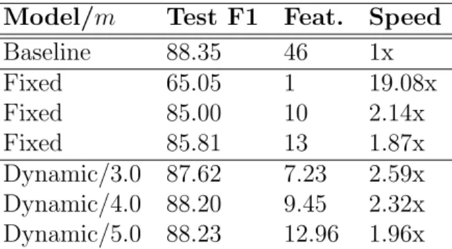
In this chapter I present paired learning and inference algorithms for significantly reducing computation and increasing speed of the vector dot products in the classifiers that are at the heart of many NLP components. This is accomplished by partitioning the features into a sequence of templates which are ordered such that high confidence can often be reached using only a small fraction of all features. Parameter estimation is arranged to maximize accuracy and early confidence in this sequence. Our approach is simpler and better suited to NLP than other related cascade methods. We present experiments in left-to-right part-of-speech tagging, named entity recognition, and transition-based dependency parsing. On the typical benchmarking datasets we can preserve POS tagging accuracy above 97% and parsing LAS above 88.5% both with over a five-fold reduction in run-time, and NER F1 above 88 with more than 2x increase in speed.
2.1
Introduction
This chapter describes a paired learning and inference approach for significantly reducing computation and increasing speed while preserving accuracy in the linear classifiers typically used in many NLP tasks. The heart of the prediction computation in these models is a dot-product between a dense parameter vector and a sparse feature vector. The bottleneck in these models is then often a combination of feature extraction and numerical operations, each of which scale linearly in the size of the
feature vector. Feature extraction can be even more expensive than the dot products, involving, for example, walking sub-graphs, lexicon lookup, string concatenation and string hashing. We note, however, that in many cases not all of these features are necessary for accurate prediction. For example, in part-of-speech tagging if we see the word “the,” there is no need to perform a large dot product or many string operations; we can accurately label the word aDeterminerusing the word identity feature alone. In other cases two features are sufficient: when we see the word “hits” preceded by a Cardinal (e.g. “two hits”) we can be confident that it is a Noun.
We present a simple yet novel approach to improve processing speed by dynam-ically determining on a per-instance basis how many features are necessary for a high-confidence prediction. Our features are divided into a set of feature templates, such as current-token or previous-tag in the case of POS tagging. At training time, we determine an ordering on the templates such that we can approximate model scores at test time by incrementally calculating the dot product in template ordering. We then use a running confidence estimate for the label prediction to determine how many terms of the sum to compute for a given instance, and predict once confidence reaches a certain threshold.
In similar work, cascades of increasingly complex and high-recall models have been used for both structured and unstructured prediction. Viola and Jones (2001) use a cascade of boosted models to perform face detection. Weiss and Taskar (2010) add increasingly higher-order dependencies to a graphical model while filtering the output domain to maintain tractable inference. While most traditional cascades pass instances down to layers with increasingly higher recall, we use a single model and accumulate the scores from each additional template until a label is predicted with suf-ficient confidence, in a stagewise approximation of the full model score. Our technique applies to any linear classifier-based model over feature templates without changing the model structure or decreasing prediction speed.
Most similarly to our work, Weiss and Taskar (2013) improve performance for several structured vision tasks by dynamically selecting features at runtime. However, they use a reinforcement learning approach whose computational tradeoffs are better suited to vision problems with expensive features. Obtaining a speedup on tasks with comparatively cheap features, such as part-of-speech tagging or transition-based parsing, requires an approach with less overhead. In fact, the most attractive aspect of our approach is that it speeds up methods that are already among the fastest in NLP.
We apply our method to left-to-right part-of-speech tagging in which we achieve accuracy above 97% on the Penn Treebank WSJ corpus while running more than five times faster than our 97.2% baseline. We also achieve a five-fold increase in transition-based dependency parsing on the WSJ corpus while achieving an LAS just 1.5% lower than our 90.3% baseline. Named entity recognition also shows significant speed increases. We further demonstrate that our method can be tuned for 2.5−3.5x multiplicative speedups with nearly no loss in accuracy.
2.2
Classification and Structured Prediction
Our algorithm speeds up prediction for multiclass classification problems where the label set can be tractably enumerated and scored, and the per-class scores of input features decompose as a sum over multiple feature templates. Frequently, classifica-tion problems in NLP are solved through the use of linear classifiers, which compute scores for input-label pairs using a dot product. These meet our additive scoring criteria, and our acceleration methods are directly applicable.
However, in this work we are interested in speeding upstructured prediction prob-lems, specifically part-of-speech (POS) tagging and dependency parsing. We apply our classification algorithms to these problems by reducing them to sequential pre-diction (Daum´e III et al., 2009). For POS tagging, we describe a sentence’s part