Coupling Dynamic Load Balancing with Asynchronism in Iterative Algorithms
on the Computational Grid
∗Jacques M. Bahi, Sylvain Contassot-Vivier and Rapha¨el Couturier
Laboratoire d’Informatique de Franche-Comt´e (LI FC),
IUT de Belfort-Montb´eliard, BP 27, 90016 Belfort, France
Abstract
In a previous work, we have shown the very high power of asynchronism for parallel iterative algorithms in a global context of grid computing. In this article, we study the inter-est of coupling load balancing with asynchronism in these algorithms. We propose a non-centralized version of dy-namic load balancing which is best suited to asynchronism. After showing, by some experiments on a given ODE prob-lem, that this technique can efficiently enhance the perfor-mances of our algorithms, we give some general conditions for the use of load balancing to obtain good results with this kind of algorithms.
Introduction
In the context of scientific computations, iterative algo-rithms are very well suited for a large class of problems and are in many cases either preferred to direct methods or even sometimes the single way to solve the problem. Di-rect algorithms give the exact solution of a problem within a finite number of operations whereas iterative algorithms provide an approximation of it, we say that they converge (asymptotically) towards this solution. When dealing with very great dimension problems, iterative algorithms are pre-ferred especially if they give a good approximation in a little number of iterations.
These last properties have led to a good expansion of parallel iterative algorithms. Nevertheless, most of these parallel versions are synchronous. We have shown in [3] all the interest of using asynchronism in such parallel iterative algorithms especially in a global context of grid computing. Moreover, in another work [2], we have also shown that static load balancing can sharply improve the performances of our algorithms.
In this article, we discuss the general interest of using dy-namic load balancing in asynchronous iterative algorithms and we show with some experiments its major efficiency ∗This research was supported by the STIC Department of the CNRS
in the global context of grid computing. Due to the nature of these algorithms, a centralized version of load balancing would not be well suited. Hence, the technique used in this study works locally between neighboring processors. The neighborhood in our case is determined by the communi-cations between processors. Two nodes are defined to be neighbors if they have to exchange data to perform their job. To evaluate the gain brought by this technique, some exper-iments are performed on the brusselator problem [8] which is described by an Ordinary Differential Equation (ODE).
The following section recalls the principle of asyn-chronous iterative algorithms and replaces them in the context of parallel iterative algorithms. Then, Section 2 presents a small discussion about the motivations of us-ing load balancus-ing in such algorithms. A brief overview of related works concerning non-centralized load balancing techniques is given in Section 3. An example of applica-tion is exhibited with the Brusselator problem detailed in Section 4. The corresponding algorithm and the insertion of load balancing are then detailed in Section 5. Finally, experimental results are given and interpreted in Section 6.
1
What are asynchronous iterative
algo-rithms ?
1.1
Iterative algorithms: backgrounds
Iterative algorithms have the structure
xk+1=g(xk), k= 0,1, ... withx0given (1)
where each xk is an n - dimensional vector, and g is some function fromIRn into itself. If the sequencexk generated by the above iteration converges to somex∗and ifgis continuous then we havex∗=g(x∗),we say thatx∗ is a fixed point ofg.
Let xk be partitioned into m block-components Xk
i, i ∈ {1, ..., m}, and g be partitioned in a
(1) can be written as Xk+1 i =Gi Xk 1, ..., Xmk i= 1, ..., m, withX0given (2) and the iterative algorithm can be parallelized by let-ting each of the m processors update a different block-component ofxaccording to (2) (see [12]). At each stage, theithprocessor knows the value of all components ofXk on whichGidepends, computes the new valuesXik+1,and communicates those on which other processors depend to make their own iterations. The communications required for the execution of iteration (2) can then be described by means of a directed graph called the dependency graph.
Iteration (2) in which all the components of xare si-multaneously updated, is called a Jacobi - type iteration. If the components are updated one at a time and the most re-cently computed values are used, then the iteration is called a Gauss-Seidel iteration. We see that Jacobi algorithms are suitable for parallelization and that Gauss-Seidel algorithms may converge faster than Jacobi ones but may be completely non-parallelizable (for example if everyGi depends on all componentsXj).
1.2
A categorization of parallel iterative
algo-rithms
Since this article deals with what we commonly call asynchronous iterative algorithms, it appears necessary, for clarity, to detail the class of parallel iterative algorithms. This class can be decomposed in three main parts:
Synchronous Iterations - Synchronous Communica-tions(SISC) algorithms: all processors begin the same iter-ation at the same time since data exchanges are performed at the end of each iteration by synchronous global com-munications. After parallelization of the problem, these algorithms have exactly the same behavior as the sequen-tial version in terms of the iterations performed. Hence, their convergence is directly deducible from the initial al-gorithm. Unfortunately, the synchronous communications strongly penalize the performance of these algorithms. As can be seen in Figure 1, there may be a lot of idle times (white spaces) between iterations (grey blocks) depending on the speed of communications.
Synchronous Iterations - Asynchronous Communica-tions (SIAC) algorithms: all processors also wait for the receipts of needed data updated at the previous iteration to begin the next one. Nevertheless, each data (or group of data) required on another processor is sent asynchronously as soon as it has been updated in order to overlap its com-munication by the remaining computations of the current iteration. This scheme lies on the probability that data will be received on the destination processor before the end of the current iteration, and then will be directly available for
the next iteration. Hence, this partial overlapping of com-munications by computations during each iteration implies shorter idle times and then better performances. Since each processor begins its next iteration as soon as it has received all its needed data updated from the previous iteration, all the processors may not begin their iterations at the same time. Nonetheless, in terms of iterations, the notion of syn-chronism still holds in this scheme since at any time t, it is not possible to have two processors performing different iterations. In fact, at eacht, processors are either comput-ing the same iteration or idle (waitcomput-ing for data). Hence, as well as the SISC, this category of algorithms performs the same iterations as the sequential version, from the algo-rithmic point of view, and have then the same convergence properties. Unfortunately, this scheme does not completely eliminate idle times between iterations, as shown in Fig-ure 2, since some communications may be longer than the computation of the current iteration and also because the sending of the last updated data on the latest processor can not be overlapped by computations.
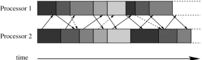
Asynchronous Iterations - Asynchronous Communi-cation(AIAC) algorithms: all processors perform their iter-ations without taking care of the progress of the other pro-cessors. They do not wait for predetermined data to become available from other processors but they keep on computing, trying to solve the given problem with whatever data hap-pen to be available at that time. Since the processors do not wait for communications, there is no more idle times be-tween the iterations as can be seen in Figure 3. Although widely studied theoretically, very few implementations and experimental analysis have been carried out, especially in the context of grid computing. In the literature, there are two algorithmic models corresponding to these algorithms, the Bertsekas and Tsitsiklis model [5] and the El Tarazi’s model [11]. Nevertheless, several variants can be deduced from these models depending on when the communications are performed and when the received data are incorporated in the computations, see e.g. [4, 1]. Figure 3 depicts a gen-eral version of an AIAC with a data decomposition in two halves for the asynchronous sendings. This type of algo-rithms requires a meticulous study to ensure their conver-gence because even if a sequential iterative algorithm con-verges to the right solution, its asynchronous parallel coun-terpart may not converge. It is then needed to develop new converging algorithms and several problems appear like choosing the good criterion for convergence detection and the good halting procedure. There are also some implemen-tation problems due to the asynchronous communications which imply the use of an adequate programming environ-ment. Nevertheless, despite all these obstacles, these algo-rithms are quite convenient to implement and are the most efficient especially in a global context of grid computing as we have already shown in [3]. This comes from the fact that
they allow communication delays to be substantial and un-predictable which is a typical situation in large networks of heterogeneous machines.
time Processor 2 Processor 1
Figure 1. Execution flow of a SISC algorithm with two processors.
time Processor 2 Processor 1
Figure 2. Execution flow of a SIAC algorithm with two processors. In this example, the first half of data is sent as soon as updated and the second half is sent at the end of the iteration.
time Processor 2 Processor 1
Figure 3. Execution flow of an AIAC algorithm with two processors. Dashed lines represent the communications of the first half of data, and solid lines are for the second half.
2
Why using load balancing in AIAC ?
The scope of this paper is to study the interest of load bal-ancing in the AIAC model. One of our goals is to show that, contrary to a generally accepted idea, asynchronism does not exempt from balancing the workload. Indeed, the load balancing can efficiently take into account the heterogeneity of the machines involved in the parallel iterative computa-tion. This heterogeneity can be found at the hardware level when using machines with different speeds but also at the user level if the machines are used in users or multi-tasks contexts. All these cases are especially encountered when dealing with grid computing.
Moreover, even in a homogeneous context, this coupling has the great advantage to deal with the evolution of the
computation during the iterative process. In numerous prob-lems resolved by iterative algorithms, the progression to-wards the solution is not the same for all the components of the system and some of them reach the fixed point faster than others. By performing a load balancing with some cri-teria based on this progression (the residual for example), it is then possible to enhance the repartition of the actually evolving computations over the processors.
Hence, there are two main ideas motivating the coupling of load balancing and AIAC algorithms:
• when the workload is well balanced on the distributed system, asynchronism allows to efficiently overlap communications by computations, especially on net-works with very fluctuating latencies and/or band-widths.
• even if AIACs are potentially more efficient than the other models, they do not take into account the work-load repartition over the processors. If this is well man-aged, it can reasonably make us expect yet better per-formances.
The great advantage of AIACs in this context is that they are far more flexible than synchronous ones in the way that it is less imperative to have at all times exactly the same amount of work on each processors. The goal here is then to avoid too large differences of progress between processors. A non-centralized strategy of load balancing appears to be best suited since it avoids global communications which would synchronize the processors. Also, it allows an adap-tive load balancing strategy according to the local context.
3
Non-centralized load balancing models
The load balancing problem has been widely studied from different perspectives and in different contexts. A cat-egorization of the various techniques for load balancing can be found in [9] based on criteria like centralized/distributed, static/dynamic, and synchronous/asynchronous. To be con-cise, we present here the few techniques which are the most suited to AIAC algorithms.
In the context of parallel iterative computations, the schedule of load balancing must be non-centralized and it-erative by nature. Local itit-erative load balancing algorithms were first proposed by Cybenko in [7]. These algorithms iteratively balance the load of a node with its neighbors until the whole network is globally balanced. There are mainly two iterative load balancing algorithms: diffusion algorithms [7] and their variants, the dimension exchange algorithms [9, 7]. Diffusion algorithms assume that a pro-cessor simultaneously exchanges load with its neighbors, whereas dimension exchange algorithms assume that a pro-cessor exchanges load with only one neighbor (along each dimension or link) at each time step.
Unfortunately, these techniques are all synchronous which is not convenient for the AIAC class of algorithms. Bertsekas and Tsitsiklis have proposed in [5] an asyn-chronous model for iterative non-centralized load balanc-ing. The principle is that each processor has an evaluation of its load and those of all its neighbors. Then, at some given times, this processor looks for its neighbors which are less loaded than itself. Finally, it distributes a part of its load to all these processors. A variant evoked by the authors is to send a part of the work only to the lightest loaded neighbor. This last variant has been chosen for implementation in our AIAC algorithms since it has the most suited properties: it maintains the asynchronism in the system with only local communications between two neighboring nodes.
In the following section, we describe a typical problem of Ordinary Differential Equations (ODEs) which has been chosen for our experimentations, the Brusselator problem.
4
The Brusselator problem
In this section, we present the Brusselator problem which is a large stiff system of ODEs. Thus, as pointed by Bur-rage [6], the use of implicit methods is required and then, large systems of nonlinear equations have to be solved at each iteration. Obviously, it can be seen that parallelism is natural for such kind of problems.
The Brusselator system models a chemical reaction mechanism which leads to an oscillating reaction. It deals with the conversion of two elementsAandBinto two oth-ersCandDby the following series of steps:
A → X
2X+Y → 3Y B+X → Y +C
X → D
(3)
There is an autocatalysis and when the concentrations of A and B are maintained constant, the concentrations ofX andY oscillate with time. For any initial concentrations of X andY, the reaction converges towards what is called the limit cycle of the reaction. This is the graph representing the concentration ofXagainst those ofY and it corresponds in this case to a closed loop.
The desired results are the evolutions of the concentra-tionsuandvof both elementsXandY along the discretized space in function of time. If the discretization is made with N points, the evolution of theuiandvifori = 1, ..., N is given by the following differential system:
u
i= 1 +u2ivi−4ui+α(N+ 1)2(ui−1−2ui+ui+1)
v
i= 3ui−u2ivi+α(N+ 1)2(vi−1−2vi+vi+1)
(4) The boundary conditions are:
u0(t) = uN+1(t) = α(N+ 1)2
v0(t) = vN+1(t) = 3
and initial conditions are:
ui(0) = 1 +sin(2πxi) with xi= Ni+ 1, i= 1, ..., N vi(0) = 3
Here, we fix the time interval to[0,10]andα= 501.Nis a parameter of the problem.
For further information about this problem and its for-mulation, the reader should refer to [8].
5
AIAC algorithm and load balancing
In this section, we consider the use of a network of workstations composed ofNbP rocsmachines (processors, nodes...) numbered from0toNbP rocs−1. Each processor can send and receive data from any other one.
It must be noticed that the principle of AIAC algorithms is generic and can be adapted to every iterative proces-sus under convergence hypotheses which are satisfied for a large class of problems. In most cases, the adaptation comes from the data dependencies, the function to approx-imate and the methods used for intermediate computations. By this way, these algorithms can be used to solve either linear or non-linear systems which can be stationary or not. In the case of the Brusselator problem, theuiandviof the system are represented in a single vector as follows:
y= (u1, v1, ..., uN, vN) withui=y2i−1andvi=y2i,i∈ {1, ..., N}.
Theyj functions,j ∈ {1, ...,2N}thereby defined will also be referred to as spatial components in the remaining of the article.
5.1
The AIAC algorithm solving the Brusselator
problem
To solve the system (4), we use a two-stage iterative al-gorithm:
• At each iteration:
– use the implicit Euler algorithm to approximate the derivative,
– use the Newton algorithm to solve the resulting nonlinear system.
The inner procedure will be calledSolvein our algorithm. In order to exploit the parallelism, theyj functions are ini-tially homogeneously distributed over the processors. Since these functions are represented in a one dimensional space (the state vectory), we have chosen to logically organize our processors in a linear way and map the spatial com-ponents (yj functions) over them. Hence, each processor
applies the Newton method over its local components us-ing the needed data from other processors involved in its computations. From the Brusselator problem formulation, it arises that the processing of components yp to yq also depends on the two spatial components beforeypand the two spatial components afteryq. Hence, if we consider that each processor owns at least two functionsyj, the non-local data needed by each processor to perform its iterations come only from the previous processor and the following one in the logical organization. In practical cases, there will be much more than two functions over each node.
In Algorithm 1, the core of the AIAC algorithm without load balancing is presented. Since the convergence detec-tion and halting procedure are not directly involved in the modifications brought by the load balancing, only the iter-ative computations and corresponding communications are detailed.
In this algorithm, the arraysYnewandYold have al-ways the following organization: the two last components from the left neighbor, the local components of the node and the two first components of the right neighbor. This struc-ture will have to be maintained even when performing load balancing. TheStartCandEndC variables are used to indicate the beginning and the end of the local components actually computed by the node. Finally, theδtvariable rep-resents the precision of the time discretization needed to compute the evolution of spatial components in time.
In order to facilitate and enhance the implementation of asynchronous communications, we have chosen to use the PM2multi-threaded programming environment [10]. This kind of environment allows to make the send and receive operations in additional threads rather than in the main pro-gram. This is why the receipts of data do not directly appear in our algorithms. In fact, they are localized in functions called by a thread created at beginning of the program and dealing with incoming messages. Thus, when a sending op-eration is performed over a given processor, it must be spec-ified which function over the destination node will manage the message. In the same way, the asynchronous sending operations appearing in our algorithms actually correspond to the creation of a communication thread calling the related sending function.
Receive functions given in Algorithms 2 and 3 only con-sist in receiving two components from the corresponding neighbor (left or right) and put them at the right place, be-fore or after the local components, in array Ynew. It can be noticed that all the variables in Algorithm 1 can be directly accessed by the receive functions since they are in threads which share the same memory space.
For each communication function (send or receive), a mutual exclusion system is used to avoid simultaneous threads to perform the same kind of communication with different data which could lead to incoherent situations and
Algorithm 1Unbalanced AIAC algorithm Initialize the communication interface NbProcs =Number of processors MyRank =Rank of the processor
Yold, Ynew =Arrays of local spatial components StartC, EndC =Indices of the first and last local spatial components
ReT =Range of evolution time of the spatial components StartT, EndT =First (0) and last (ReT/δt) values of time Initialization of local data
repeat
forj=StartCtoEndCdo fort=StartTtoEndTdo
Ynew[j,t] = Solve(Yold[j,t])
end for
ifj=StartC+2andMyRank>0then
ifthere is no left communication in progressthen
Send asynchronously the two first local com-ponents to left processor
end if end if end for
ifMyRank<NbProcs-1then
ifthere is no right communication in progressthen
Send asynchronously the two last local compo-nents to right processor
end if end if
Copy Ynew in Yold
untilGlobal convergence is achieved Display or save local components Halt the communication system
Algorithm 2function RecvDataFromLeft() Receive two components from left node
Put these components before local components in array Yold
Algorithm 3function RecvDataFromRight() Receive two components from right node
Put these components after local components in array Yold
also to useless overloading of the network. This has also the advantage to generate less communications. Hence, the AIAC variant used here and detailed in Figure 4 is slightly different from the general case given in Figure 3.
time Processor 2 Processor 1
Figure 4. Execution flow of our AIAC variant with two processors. Dashed lines represent communications which are not actually per-formed due to mutual exclusion. Solid lines starting during iterations corresponds to left sendings whereas those at the end of itera-tions are for right ones.
5.2
Load balanced version of the AIAC algorithm
As evoked in Section 3, Bertsekas et al. have proposed a theoretical algorithm to perform load balancing asyn-chronously and have proved its convergence. We have used this model to design our load balancing algorithm adapted to parallel iterative algorithms and particularly to AIACs on the grid. Each processor will periodically test if it has to balance its load with one of its neighbors, the left or the right here. If needed, it will send a given amount of data to its lightest loaded neighbor.
In Algorithm 4 is presented the load balanced version of the AIAC algorithm given in Section 5.1. For clarity, im-plementation details which are relative to the programming environment used are not shown.
Most of the additional parts take place at the beginning of the main loop. At each iteration, we test if a load bal-ancing process has been performed. If it is the case, data arrays have to be resized in order to contain just the local components affected to the node. Hence, a second test is performed to see if the node has received or sent data. In the former case, the arrays have to be enlarged in order to receive the additional data which have then to be copied in this new array. In the latter, arrays have to be reduced and no data copying is necessary.
If no load balancing has been performed, several things have to be tested to perform a load balancing towards the left or right processor. The first one allows us to try load balancing periodically at everykiterations. This is useful to tune the frequency of load balancing during the iterative process which directly depends on the problem considered. In some cases, a high frequency will be efficient whereas in other cases lower frequencies will be recommended since
too much load balancing could take the most computation time of the process according to the iterations, especially with low bandwidth networks.
The second test detects if a communication from a previ-ous load balancing is not finished yet. In this case, the trial is delayed to the next iteration and so on until the previous communication is achieved. In the other case, the corre-sponding function is called.
It can be noticed that according to the current organiza-tion of these tests, the left load balancing is tested before the right which could seem to advantage it. In fact, this is not actually the case and this does not alter the generality of our algorithm. This has only been done to avoid simultaneous load balancings of a processor with its two neighbors which would not conform to the model used.
Finally, the last point in the main algorithm concerns the data sendings performed at each iteration. Since the arrays may change from an iteration to another, we have to ensure that the received data correspond to the local data before (/after) the current arrays and can then be safely put before (/after) them. This is why the global position of the two first (/last) components are joined to the data. Moreover, in order to decide whether or not to balance the load, the local resid-uals are used and then sent together with the components. It may seem surprising to use the residual as a load estimator but this choice is very well adapted to this kind of computa-tion as exposed in Seccomputa-tion 2. At first sight, everyone could think that taking, for example, the time to perform theklast iterations would give a better criterion. Nevertheless, the lo-cal residual allows us to take into account the advance of the current computations on a given processor. So, if a proces-sor has a low residual, all its components are not evolving so far and its computations are not so useful for the over-all progression of the algorithm. Hence, it can then receive more components to treat in order to potentially increase its usefulness and also allow its neighbor to progress faster.
In Algorithm 5 is detailed the function to balance the load with the left neighbor. Obviously, this function has its symmetrical version for the right neighbor. Its first step is to test if a balancing is actually needed by computing the ratio of the residuals on the two processors and comparing it to a given threshold. If satisfied, the number of data to send is then computed and another test is done to verify that the number of data remaining on the processor will be large enough. This is done to avoid the famine phenomenon on slowest processors. Finally, the computed number of the first (/last) data are asynchronously sent with two more components which will represent the dependencies of the left (/right) processor. These two additional data will con-tinue to be computed by the current processor but their val-ues will be sent to the left (/right) processor to allow it to perform its own computations with updated values of its data dependencies. In the same way, the two components
Algorithm 4Load balanced AIAC algorithm Initialize the communication interface Variables from Algorithm 1
LBDone = boolean indicating if LB has just been per-formed
LBReceipt =boolean indicating if additional data from LB have been received
OkToTryLB = integer allowing to periodically test for performing LB. Initially set to 20
Initialization of local data
repeat
ifLBDone=truethen ifLBReceipt=truethen
Resize Ynew,Yold arrays after receipt of addi-tional data
Complete new Yold array with additional data from temporary array
LBReceipt=false
else
Resize Ynew,Yold arrays after sending of trans-ferred data
end if
LBDone=false
else
ifOkToTryLB=0then
ifthere is no left LB communication in progress
then
TryLeftLB()
else
if there is no right LB communication in progressthen TryRightLB() end if end if else OkToTryLB=OkToTryLB-1 end if end if
forj=StartCtoEndCdo
... /* ... indicate the same parts as in Algorithm 1 */ Send asynchronously the two first local
components and the residual of previous iteration preceded by their global position to left processor ...
end for
...
Send asynchronously the two last local
components and the residual of current iteration preceded by their global position to right processor ...
untilGlobal convergence is achieved ...
before (/after) those two ones will be kept on the current processor and become its data dependencies from the left (/right) neighbor.
Algorithm 5function TryLeftLB() /* symmetrical for TryRightLB() */
Ratio =Ratio of residuals between local node and its left neighbor
NbLocal =Number of local data
NbToSend =Number of data to send to perform LB Ratio=local residual / left residual
ifRatio>ThresholdRatiothen
Compute the number of data to send NbToSend
ifNbLocal-NbToSend>ThresholdDatathen
Send asynchronously the NbToSend+2 first data to left processor
/* +2 added for data dependencies */ OkToTryLB=20
LBDone=true
end if end if
Concerning the receipt functions, the first kind, exhibited in Algorithm 6, is related to the load balancing whereas the second type, given in Algorithm 7, deals with the classical data exchanges induced by dependencies. The former func-tion consists in placing addifunc-tional data into a temporary ar-ray until they are copied in the resized arar-ray Yold, after what the temporary array is destroyed. Once the receipt is done, the flags indicating the completion of a load balancing com-munication and its nature are set. The latter function has the same role as the one presented in Algorithm 2. Nonetheless, in this version, the global position of the received data must be confronted to the expected one before stocking them in the array. Also, the residual obtained on the source node is an additional data to receive.
Algorithm 6function RecvDataFromLeftLB() /* symmetrical for RecvDataFromRightLB() */ Receive the number of additional data sent
Receive these data and put them in a temporary array LBReceipt=true
LBDone=true
Finally, we obtain a load balanced AIAC algorithm which solves the Brusselator problem.
6
Experiments
In order to perform our experiments, we have used the PM2 (Parallel Multi-threaded Machine) environment [10]. Its first goal is to efficiently support irregular parallel ap-plications on distributed architectures. We have already
Algorithm 7function RecvDataFromLeft() /* symmetrical for RecvDataFromRight() */
ifnot accessing data arraythen
Receive the global position and the two components from left node
if global position corresponds to the two left data needed on local nodethen
Put these data before local components in array Yold
else
Do not stock these data in array Yold /* array Yold is being resized */
end if
Receive the residual obtained on the left node
end if
shown in [3] the convenience of this kind of environment for programming asynchronous iterative algorithms in a global context of grid computing.
In order to evaluate the gain obtained by coupling load balancing with asynchronism, the balanced and non-balanced versions of our AIAC algorithm are compared in two different contexts. The former is a local homogeneous cluster with a fast network and the latter is a collection of heterogeneous machines scattered on distant sites. In this last context, the machines were subject to a multi-users uti-lization directly influencing their load. Hence, our results correspond to the average of a series of executions.
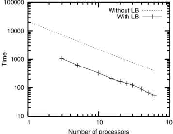
Figure 5 shows the evolution of execution times in func-tion of the number of processors on a local homogeneous cluster. It can be seen that both versions have a very good scalability. This is a quite important point since load bancing usually introduces sensitive overheads in parallel al-gorithms leading to quite moderate scalabilities. This good result mainly comes from the non-centralized nature of the balancing used in our algorithm. Nevertheless, the most in-teresting point is the large vertical offset between the curves which denotes a high gain in performances. In fact, the ratio of execution times between the non-balanced and balanced versions varies from 6.2 to 7.4 with an average of 6.8. These results show all the efficiency of coupling load balancing with AIAC algorithms on a local cluster of homogeneous machines.
Concerning the heterogeneous cluster, fifteen machines have been used over three sites in France: Belfort, Montb´eliard and Grenoble, between which the speed of the network may sharply vary. The logical organization of the system has been chosen irregular in order to get a grid com-puting context not favorable to load balancing. The machine types vary from a PII 400Mhz to an Athlon 1.4Ghz. The re-sults obtained are given in Table 1.
Here also, the balancing brings an impressive enhance-ment to the performances of the initial AIAC algorithm.
10 100 1000 10000 100000 1 10 100 Time Number of processors Without LB With LB
Figure 5. Execution times (in seconds) on a homogeneous cluster
version non-balanced balanced ratio execution time 515.3 105.5 4.88 Table 1. Execution times (in seconds) on a heterogeneous system
The smaller ratio than in local cluster is explained by the larger cost of communications and then of data migrations. Although this ratio stays very satisfying, this remark would imply a closer study concerning the tuning of the load bal-ancing frequency during the iterative process. This is not in the scope of this article but will probably be the subject of a future work.
Despite this, the load balancing is more interesting in this context than in local clustering. This comes from the fact that in the homogeneous context, as was shown in [3], the synchronous and asynchronous iterative algorithms have al-most the same behavior and performances whereas in the global context of grid computing, the asynchronous version reveals all its interest by providing far better results. Hence, we can reasonably deduce that load balancing AIAC algo-rithms in a local homogeneous context would only produce slightly better results than their SISC counterparts whereas in the global context, the difference between SISC and AIAC load balanced versions will be much larger. In fact, this last version will obtain the very best performances.
As explained in Section 2 and pointed out by these ex-periments, load balancing and asynchronism are then not incompatible and can actually lead to very efficient parallel iterative algorithms.
this coupling is performed but also the context in which it is used. The first point has already been discussed and it has been showed the important role played by the non-centralized nature of the balancing technique. Concern-ing the second point, there are also some conditions which should be verified on the treated problem to ensure good performances.
According to our experiments, it has appeared at least four conditions required to get an efficient load balancing on asynchronous iterative algorithms. The first one con-cerns the number of iterations which must be large enough to make it worth to perform load balancing. In the same way, the average time to perform one iteration must be long enough to have a reasonable ratio of computations over communications. In the opposite case, the load balancing will not sensibly influence the performances and will have the drawback to overload the network. Another important point is the frequency of load balancing operations which must be neither too high (to avoid an overloading of the system) nor too low (to avoid a too large imbalance in the system). It is then important to design a good measure of the need to load balance. Finally, the last point is the ac-curacy of the load balancing which depends on the network load. If the network is heavily loaded (or slow) it may be preferable to perform a coarse load balancing with less data migration. On the other hand, an accurate load balancing will tend to speed up the global convergence. The tricky work is then to find the good trade-off between these two constraints.
7
Conclusion
The general interest of load balancing parallel iterative algorithms has been discussed and its major efficiency in the context of grid computing has been experimentally shown.
A comparison has been presented between a non-balanced and a non-balanced asynchronous iterative algorithm. Experiments have been done with the Brusselator problem using the PM2 multi-threaded environment. It has been tested in two representative contexts. The first one is a local homogeneous cluster and the second one corresponds to a global context of grid computing.
The results of these experiments clearly show that the coupling of load balancing and asynchronism is fully justi-fied since it gives far better performances than asynchro-nism alone which is itself better than synchronous algo-rithms. The efficiency of this coupling comes from the fact that these two techniques individually optimize two differ-ent aspects of parallel iterative algorithms. Asynchronism brings a natural and automatic overlapping of communica-tions by computacommunica-tions and load balancing, as named, pro-vides a good repartition of the work over the processors. The advantage induced by the non-centralized nature of the
balancing technique has also been pointed out. Avoiding global synchronizations leads to less overheads and then to a better scalability.
In conclusion, balancing the load in asynchronous iter-ative algorithms can actually bring higher performances in both local and global contexts of grid computing.
References
[1] J. M. Bahi. Asynchronous iterative algorithms for nonex-pansive linear systems. Journal of Parallel and Distributed Computing, 60(1):92–112, Jan. 2000.
[2] J. M. Bahi, S. Contassot-Vivier, and R. Couturier. Evalu-ation of the asynchronous model in iterative algorithms for global computing. (in submission).
[3] J. M. Bahi, S. Contassot-Vivier, and R. Couturier. Asyn-chronism for iterative algorithms in a global computing en-vironment. InThe 16th Annual International Symposium on High Performance Computing Systems and Applications (HPCS’2002), pages 90–97, Moncton, Canada, June 2002. [4] D. E. Baz, P. Spiteri, J. C. Miellou, and D. Gazen.
Asyn-chronous iterative algorithms with flexible communication for nonlinear network flow problems. Journal of Parallel and Distributed Computing, 38(1):1–15, 10 Oct. 1996. [5] D. P. Bertsekas and J. N. Tsitsiklis.Parallel and Distributed
Computation: Numerical Methods. Prentice Hall, Engle-wood Cliffs NJ, 1989.
[6] K. Burrage. Parallel and Sequential Methods for Ordinary Differential Equations. Oxford University Press Inc., New York, 1995.
[7] G. Cybenko. Dynamic load balancing for distributed mem-ory multiprocessors. Journal of Parallel and Distributed Computing, 7(2):279–301, Oct. 1989.
[8] E. Hairer and G. Wanner.Solving ordinary differential equa-tions II: Stiff and differential-algebraic problems, volume 14 ofSpringer series in computational mathematics, pages 5–8. Springer-Verlag, Berlin, 1991.
[9] S. H. Hosseini, B. Litow, M. Malkawi, J. McPherson, and K. Vairavan. Analysis of a graph coloring based distributed load balancing algorithm. Journal of Parallel and Dis-tributed Computing, 10(2):160–166, Oct. 1990.
[10] R. Namyst and J.-F. M´ehaut. P M2: Parallel multithreaded machine. A computing environment for distributed archi-tectures. InParallel Computing: State-of-the-Art and Per-spectives, ParCo’95, volume 11, pages 279–285. Elsevier, North-Holland, 1996.
[11] M. E. Tarazi. Some convergence results for asynchronous algorithms.Numer. Math., 39:325–340, 1982.